1
Department of Neurobiology, Duke University School of Medicine, Durham, NC, USA
2
Center for Neuroeconomic Studies, Duke University, Durham, NC, USA
3
Center for Cognitive Neuroscience, Duke University, Durham, NC, USA
4
Department of Psychology, University of Illinois, Chicago, IL, USA
5
Department of Psychology and Neuroscience, Duke University, Durham, NC, USA
6
Department of Evolutionary Anthropology, Duke University, Durham, NC, USA
In most natural decision contexts, the process of selecting among competing actions takes place in the presence of informative, but potentially ambiguous, stimuli. Decisions about magnitudes – quantities like time, length, and brightness that are linearly ordered – constitute an important subclass of such decisions. It has long been known that perceptual judgments about such quantities obey Weber’s Law, wherein the just-noticeable difference in a magnitude is proportional to the magnitude itself. Current physiologically inspired models of numerical classification assume discriminations are made via a labeled line code of neurons selectively tuned for numerosity, a pattern observed in the firing rates of neurons in the ventral intraparietal area (VIP) of the macaque. By contrast, neurons in the contiguous lateral intraparietal area (LIP) signal numerosity in a graded fashion, suggesting the possibility that numerical classification could be achieved in the absence of neurons tuned for number. Here, we consider the performance of a decision model based on this analog coding scheme in a paradigmatic discrimination task – numerosity bisection. We demonstrate that a basic two-neuron classifier model, derived from experimentally measured monotonic responses of LIP neurons, is sufficient to reproduce the numerosity bisection behavior of monkeys, and that the threshold of the classifier can be set by reward maximization via a simple learning rule. In addition, our model predicts deviations from Weber Law scaling of choice behavior at high numerosity. Together, these results suggest both a generic neuronal framework for magnitude-based decisions and a role for reward contingency in the classification of such stimuli.
For one-dimensional quantities like number, time, length, and brightness that possess a natural linear order (Moyer and Landauer, 1967
; Stevens, 1986
), discrimination behavior is characterized by the distance and magnitude effects: discrimination improves as the difference in stimuli along the perceptual dimension increases, but suffers as the absolute magnitudes grow (Moyer and Landauer, 1967
; Brannon and Terrace, 1998
; Nieder and Miller, 2003
). More generally, such quantities obey Weber’s Law: the just-noticeable difference in a magnitude is proportional to the magnitude itself.
In the last several years, single unit recordings and fMRI studies have implicated neurons in the intraparietal sulcus in coding one of these quantities – number (Nieder et al., 2002
; Nieder and Miller, 2003
, 2004a
,b
; Nieder, 2005
; Nieder and Merten, 2007
; Roitman et al., 2007
). Moreover, neurons in the ventral intraparietal area (VIP) show preferential firing to specific numerosities, with tuning curve widths scaling as the logarithm of the preferred number (Nieder et al., 2002
; Nieder and Miller, 2003
; Nieder and Merten, 2007
). fMRI repetition suppression studies have largely confirmed these observations (Piazza et al., 2004
). As a result, most recent theoretical work on numerical cognition has focused on models that represent number via pools of neurons preferentially activated by specific numerosities (Dehaene and Changeux, 1993
; Zorzi and Butterworth, 1999
; Grossberg and Repin, 2003
; Verguts and Fias, 2004
; Nieder, 2005
; Verguts et al., 2005
). Such models naturally account for performance in discrimination tasks of both dot arrays and Arabic numerals, and suggest that the logarithmic widening of VIP neuron tuning curves gives rise to Weber’s Law for numerical discrimination.
By contrast, neurons in the lateral intraparietal area (LIP) were recently shown to represent the number of dots in a visual array in a graded, monotonic fashion (Roitman et al., 2007
). Notably, there were separate populations of LIP neurons that increased firing with increasing numerosity and decreased firing with increasing numerosity. Similar reciprocal neuronal coding of somatosensory stimuli has previously been observed in somatosensory cortex for vibration frequency (Miller et al., 2003
; Machens et al., 2005
). These analog codes provide a physiological basis for alternative models of magnitude discrimination, including number, without the need to invoke explicit neuronal representations of specific values (Gibbon, 1977
, 1981
; Gibbon and Church, 1981
; Gibbon and Fairhurst, 1994
).
Such analog models, proposed initially for interval timing, typically rely on one of two underlying neural codes for magnitudes. In linear models, magnitudes are represented by linearly increasing firing rates, with noise that grows in proportion to the firing rate itself. Comparisons between magnitudes are performed by taking ratios of these linear representations, with the result that discriminations between magnitudes become easier as distances between them grow (the distance effect) and harder to distinguish (for fixed difference between them) as their absolute values increase (the magnitude effect). Moreover, the assumption of a noisy internal representation with standard deviation proportional to the mean (constant coefficient of variation), dubbed the “scalar property,” gives rise to a discriminability parameter proportional to the difference in magnitudes divided by their absolute size, reproducing the Weber-Fechner discrimination law (Gibbon, 1977
, 1981
; Gibbon and Church, 1981
; Brannon et al., 2001
).
In the second class of models, magnitudes are represented by firing rates that scale with the logarithm of the underlying quantity (Gibbon, 1977
, 1981
; Gibbon and Church, 1981
) (not to be confused with the logarithmically widening tuning curves of numerosity-selective neurons). Comparisons in these models are performed by subtraction, a linear operation equivalent to taking the ratio of the original magnitudes. In addition, constant variance in the logarithmically compressed internal representation corresponds to a log-normal variance in the original quantity, with a standard deviation proportional to that quantity, thus reproducing the scalar property from the linear models. Thus, in contrast to population code models, which represent numerosity via pools of neurons selective for each number (“cardinal codes”), these models represent numerosity in graded fashion in a single neuronal firing rate (“ordinal codes”).
Given either of these noisy internal analog representations of magnitude, signal detection theory provides a principled framework for classification (Green and Swets, 1989
; Gibbon, 1981
). In signal detection theory, not only do the statistics of the underlying representation enter into the decision making process, but the costs and benefits of stimulus identification do so as well. Thus, if a “yes” response to a question about an ambiguous stimulus is rewarded twice as much as a “no,” the optimal strategy (from a reward maximization standpoint) is to respond “yes” in all cases where the stimulus is equally likely to correspond to either, and even in many cases where it is more likely to correspond to “no.” Typically, this prediction is tested in a bisection paradigm, in which subjects are asked to provide a binary classification of a quasi-continuous range of stimuli (Church and Deluty, 1977
; Meck and Church, 1983
; Platt and Davis, 1983
; Meck et al., 1985
; Roberts, 2005
; Jordan and Brannon, 2006
). Stimuli at either extreme of the range (the “anchors”) are each paired with a unique rewarded response, but intermediate stimuli are classified freely. By measuring the resulting choice function, the underlying decision process can be characterized.
Measurement of psychometric curves in the bisection paradigm results in two primary empirical findings (Gibbon, 1981
; Gibbon and Church, 1981
; Gibbon and Fairhurst, 1994
): First, points of subjective equality (PSE) for stimulus classification – stimulus magnitudes for which subjects are equally likely to produce either response – are located at the geometric mean of the two anchor values. Second, when plotted as a function of stimulus magnitude divided by PSE (a PSE-relative scale), psychometric curves for distinct pairs of anchors superimpose. The latter may be seen as a consequence of the scalar property (for either linear or logarithmic encoding schemes), since Weber’s Law predicts that ratio-based discrimination should be invariant to magnitude rescaling.
Here, we demonstrate that a discrimination model based on observed numerosity tuning curves for LIP neurons, in the absence of explicit representation of numerical value, is sufficient to reproduce the choice performance of macaques in a separate behavioral study of numerical bisection. We further predict departures from Weber’s Law at large numerosities that differentiate between linear and logarithmic encoding of numerosity. Furthermore, we show that simple reinforcement learning correctly sets the indifference point for numerical bisection in our model, without explicit knowledge of either reward history or underlying tuning functions, with important implications for classification performance in the case of unequally rewarded anchors. Together, our findings demonstrate that monotonic analog codes can support discrimination of abstract quantities like number, in addition to simple sensory stimuli like vibrotactile frequency (Machens et al., 2005
).
Neuronal Data: Implicit Discrimination
We base our model on neurophysiological data published previously (Roitman et al., 2007
). There, the authors characterized the responses of LIP neurons to arrays of dots in an implicit numerosity discrimination task (Roitman et al., 2007
). Single units (n = 53) were isolated in area LIP, and their spatial receptive fields identified, using a standard delayed-saccade paradigm. During the task, the animal was required to hold fixation on a central cue. They were then presented with a saccade target in the hemifield opposite the receptive field of the neuron. After a variable delay, a dot array of numerosity 2, 4, 8, 16, or 32 (controlled for density, element size, and total pixels) was presented in the receptive field for 400 ms. After another variable delay, monkeys shifted gaze to the target opposite the receptive field. In each block, one numerosity was selected as standard and presented on 50% of trials. On the other half of trials, cue numerosities were randomly chosen from among the four remaining values. The animal received 100 ms of juice for successful saccades following standard cues, 150 ms for successful saccades following deviants. (Both saccades were to the same location.) Since every trial resulting in a saccade was rewarded, animals did not need to attend to numerosity to maximize reward, though decreased reaction times for trials with deviant cues argue that they did so.
Behavioral Data: Numerical Bisection
To verify that our model produces psychometric curves of the form measured in behavioral studies of bisection, we compare its output to the previously-published work of Jordan and Brannon in a separate pair of monkeys (Jordan and Brannon, 2006
) (note that the monkeys in the Roitman et al., 2007
, study were numerically naïve and did not perform a bisection task). In Jordan and Brannon’s experiment, adult rhesus monkeys were first trained to recognize the number of elements in a dot display in a delayed match-to-sample (DMS) paradigm using a touch-sensitive monitor. Upon trial initiation, a stimulus consisting of a yellow rectangle containing a variable number of dot elements was presented, followed afterward by two choice stimuli (match and distractor) and the animal’s response. Correct choices were rewarded by juice delivery, and several confounding dimensions of the dot arrays (cumulative area, dot size, density) were controlled, ensuring that only numerosity remained a reliable guide to behavior.
Once animals were able to recognize individual numerosities, two stimuli (block type 1: 2 and 8, block type 2: 3 and 12) were selected as anchors and presented (with equal probability) as the cue stimulus. As in the DMS paradigm, a match and distractor were subsequently presented, always equal in numerosity to the anchor values. Correct trials of this type were again rewarded. However, on 30% of trials, an intermediate numerosity appeared as the cue (block type 1: 3–7, block type 2: 4–11), followed by dot array choices corresponding to the two anchors. This required the animal to classify a non-matching stimulus with one or the other of the two anchors. Though these trials were never rewarded, the animals nevertheless displayed systematic responses to the intermediate numerosity cues, transitioning from responses corresponding to the small anchor value to responses favoring the large anchor value as cue numerosity increased (Figure 1
B).
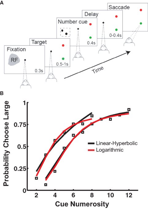
Figure 1. Numerosity bisection task. (A) Schematic showing modeled oculomotor bisection task. Following fixation, two saccade targets appear: red for “small” and green for “large.” After a variable delay, a dot array is briefly presented in the recorded neuron’s response field. Following a second variable delay, the fixation target extinguishes, and the animal makes an eye movement to either choice target in the hemifield opposite the neuron’s RF. (B) Choice behavior and model fits to a touch screen version of the numerosity bisection task (after Jordan and Brannon, 2006
). Data points represent probability of choosing the response associated with the “large” anchor value. Red and black lines indicate fits based on families of choice curves derived from the linear-hyperbolic and logarithmic encoding models. Anchor values are 2 and 8 for the left set of curves, 3 and 12 for the right.
Modeling
The most common paradigm used to study magnitude estimation and number judgment in rats, pigeons, and non-human primates is numerical bisection, in which a subject is required to classify the numerosity of a cue as one or the other of a pair of “standard” values (Church and Deluty, 1977
; Meck and Church, 1983
; Platt and Davis, 1983
; Meck et al., 1985
; Roberts, 2005
; Jordan and Brannon, 2006
). Of tasks designed to quantify numerical capability, it remains the most direct, and gives the clearest demonstration of Weber’s Law behavior. We asked whether the observed response functions of numerosity-sensitive neurons in area LIP (Roitman et al., 2007
) might function as a code capable of reproducing choice behavior in a similar bisection task.
We modeled behavior in an oculomotor version of the numerical bisection task. The oculomotor paradigm has been widely used to study response properties of LIP neurons (Snyder et al., 1997
; Andersen and Buneo, 2002
) and to probe the neural correlates of decisions in a wide variety of cognitive tasks (Platt and Glimcher, 1999
; Gold and Shadlen, 2000
; Shadlen and Newsome, 2001
; Roitman and Shadlen, 2002
; Leon and Shadlen, 2003
). Moreover, framing the experiment in this way allows us to make direct use of single-unit recordings from LIP in our model, as well as to make testable predictions about neuronal activity as task conditions are altered. In the task (Figure 1
A), fixation on the central cue is followed by the presentation of two targets (red and green) in the hemifield opposite the receptive field of a recorded neuron. This is followed by a variable delay, after which a dot array cue is presented in the neuron’s receptive field. This is followed by another variable delay, after which the animal is free to shift gaze to either the green (“small” response) or red (“large” response) target. Figure 1
B presents behavioral data from a similar bisection paradigm (Jordan and Brannon, 2006
), along with fits produced by our models (see below).
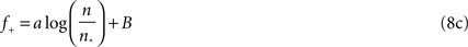
In order to extrapolate differences in model predictions to high numerosity, we fit neuronal responses of LIP during the 400 ms of stimulus presentation with both linear and logarithmic response models, each of which contained neurons that increased and decreased firing in response to increasing numerosity. (Clearly, for numerosities within the range of the measured response curves, no fitting is necessary.) In the first model, these responses followed linear-hyperbolic tuning curves:


while in the second, they followed logarithmic tuning curves:


Chi-squared values for fits to the measured mean response curves were calculated according to:
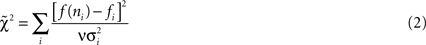
where fi are the measured firing rates, subscripts indicate positively (+) and negatively (−) monotonic responses, f(ni) are the model predictions, σi are the standard errors, and ν is the number of degrees of freedom. Noise was well fit by a Poisson process (Figure 2
D) and, for simplicity, subsequently modeled as Gaussian with equivalent first and second moments:

with  the tuning curve (either + or −) and N the normal distribution with variance . (Thus, although a real Poisson process will show deviations from this assumption, those deviations will only affect higher moments of the distribution.)
the tuning curve (either + or −) and N the normal distribution with variance . (Thus, although a real Poisson process will show deviations from this assumption, those deviations will only affect higher moments of the distribution.)
Figure 2. Single neurons in LIP monotonically encode the number of visual objects. (A) Averaged single neuron (n = 15) firing rate during the cue presentation for five different numerosities (after Roitman et al., 2007
; see Materials and Methods). Standard and deviant trials were averaged. Data are fit to a straight line. Inset shows PSTH of an example neuron for five different numerosities. Colors in the PSTH correspond to data points in the main plot. (B) Average firing rate (n = 17) for negatively monotonic neurons in LIP. Inset shows the PSTH for an example neuron. Data were fit to a hyperbolic decay. Colors are as in (A). (C) χ2 goodness-of-fit comparison between linear-hyperbolic and logarithmic models for single neurons. Black line represents equally good fits. Black squares are positively monotonic neurons, red circles negatively monotonic. Smaller χ2 values represent better fits. More symbols above the black line than below indicate the superiority of the linear-hyperbolic model as a fit to the data. (D) Coefficient of variation (mean/standard deviation) of firing rates as a function of firing rate during the 400-ms delay period following numerosity cue presentation in the implicit number task (see Materials and Methods). Each circle represents one trial for one neuron. Red line is a fit to the prediction of Poisson firing rates.
Choices were made by randomly sampling from both positive and negative tuning curves and taking differences in firing rates. As explained in the “Results” section, this firing rate difference was subsequently fed into a softmax choice model:

with PL the probability of choosing the option corresponding to the larger anchor, δf the difference in firing rates, β a parameter reflecting the variability of the animal’s choice, and a a maximum choice preference for the option with higher firing. Indifference results when δf = 0.
We simulated distinct pairs of anchor values by shifting the relative baseline firing rates (bias input) of the positive and negative tuning curves, as detailed in the “Results” sections. This resulted in a one-parameter family of psychometric choice curves, differing in their points of subjective equality (PSE). For ease of computation, we parameterized this family of choice curves by two different functional forms (our results did not depend on the choice). We fit model-generated curves with both logistic:

and Gompertz

functions. As before, a represents a maximum preference level for the large option, while n* represents the PSE and σ is a measure inversely related to discriminability. Once again, the fitting is a computational convenience, and the specific form of the parameterization does not matter. Results are unaffected if the direct outputs of the model are used instead. We fixed β and a in Eq. 4 by fitting our family of psychometric choice curves to the measured bisection behavior of monkeys in a separate experiment (Jordan and Brannon, 2006
) (Figure 1
B).
For both parameterizations of our family of choice curves, Weber’s Law predicts:

with k a constant.
We modeled the process of learning the indifference point for bisection via a reinforcement learning algorithm that tracked the values of each of the two responses and updated these along with a “bias input” favoring either the “large” or “small” response. In this case, we parameterized our tuning functions as:

for the linear-hyperbolic case and
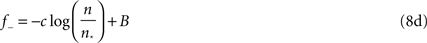
in the logarithmic case, with n* clearly equal to the point of subject equality (adjusted by the learning algorithm) and B a constant baseline firing rate common to both types of neurons. On each trial, either the large or small anchor was presented with equal probability, and the system made its response according to the output of the current decision model for the current value of n*. As in the standard bisection task, only correct answers were rewarded. Subsequent to reward, the system performed the following updates for the action values corresponding to the two choices and the PSE:
with QL the action value of choosing “large,” QS the action value of choosing “small,” R the reward outcome (either 0 or 1, for incorrect or correct) and α and λ learning rates. Note that only the value corresponding to the chosen action is updated, though the PSE changes each trial. In this way, the PSE is adjusted upward (biasing toward the “large” response) if QL > QS – in other words, in the direction of choosing the more profitable option. Clearly, equilibrium corresponds to equality of the two action values, at which point the animal should be indifferent, and reward is maximized. We report simulations performed for 15000 trials with both α and λ equal to 0.05. The initial value of the indifference point was set to the arithmetic mean of the anchors, though choosing either extreme worked equally well. Learning for most pairs of anchor values converges within 2000 trials, though mean PSEs and standard deviations were calculated over the last 4000 trials of simulation to ensure that learning had reached asymptote.
The Model Predicts Bisection Behavior in the Absence of Explicit Numerosity Codes
To model the response properties of neurons in LIP, we made use of single-unit neural activity recorded during an implicit numerosity discrimination task (see Materials and Methods). As shown in Figures 2
A,B, firing rates in these neurons varied in both positively (n = 15/53) and negatively (n = 17/53) monotonic fashion with cue numerosity. Following previous theories of magnitude discrimination, we fit these neural response functions to two models (Figures 2
A,B): In the first, the increasing response is modeled as linear (f+ = an + b, a = 1.14, b = 45.2, χ2 = 1.38), while the decreasing response is fit to a hyperbolic function (f− = c/n + d, c = 30.7, d = 37.5, χ2 = 1.18). This hyperbolic coding, not previously proposed for number, resembles that observed in primate superior colliculus when multiple, equally likely saccade targets are presented, and suggests, at least in part, an effective compression of one-half the internal representation of large numerosities (Basso and Wurtz, 1997
).
In addition, we fit neuronal responses as logarithmically encoding numerosity (f+ = a logn + b, a = 9.01, b = 40.20, χ2 = 7.40; f− = − c logn + d, c = 5.34, d = 54.6, χ2 = 1.26). Clearly, both models reproduce the negatively monotonic curve well, though the logarithmic fit in the case of the increasing response function is somewhat less convincing (Figure 2
C). However, since the logarithmic model possesses a number of interesting theoretical features and serves as an important contrast to the behavior of the linear-hyperbolic model, we report the results of our decision model in both cases. It is also important to note that such fits are only for computational convenience and the extrapolation of our predictions to high numerosity. Direct use of the empirical tuning curves produces equivalent behavior in our model over the range of numerosities tested. We also examined the variability of neuronal responses. As shown in Figure 2
D, firing rates across the population were well fit by an assumption of Poisson noise (R2 = 0.92), providing evidence against the scalar variance assumption of linear models for magnitude encoding.
A schematic for our decision model is presented in Figure 3
A. We treat the decision process as a competition between two representations, one with positive response function, one with negative, to a dot array stimulus. Similar to models of interval discrimination (Gibbon, 1977
, 1981
; Gibbon and Fairhurst, 1994
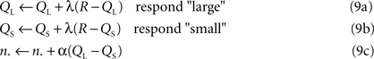
), we sample from Poisson distributions of firing centered about these response curves, calculating the difference in firing between them. In this framework, high firing rates in positively monotonic neurons give evidence for a large encoded numerosity (and thus argue for a “large” response), whereas high firing in negatively monotonic neurons argues for a small numerosity in the stimulus. The difference between these two pieces of evidence then becomes the overall bias toward the “large” response. Mathematically, this is given by the difference in the two tuning curves (see Eqs. 8a,b in Materials and Methods):
where n* is the PSE. Clearly, this number is negative for many values of n*, which case it represents either an inhibition of positively-tuned neurons or an upward shift of the negatively monotonic tuning curve. Clearly, this difference is unaffected if both firing rate responses are increased by the same amount, though such an overall shift does affect the amount of Poisson noise (and thus the variability of the signal).
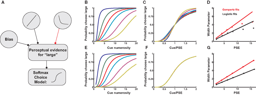
Figure 3. Two models for numerosity bisection. (A) In both models, positive and negative neuronal responses from LIP neurons enter as evidence for “large” and “small” cue classifications, respectively. In addition, a bias input represents an additional propensity to choose one response over the other. In the figure, black lines represent excitation, red lines inhibition. The bias input augments the probability of perceiving the cue as “large,” though in other cases it might favor a “small” outcome. Competition between the two tuning curves computes an effective difference in firing rates, which is passed on to a softmax choice model that apportions choices based on this difference (see Materials and Methods). (B) A family of choice curves generated by systematically decreasing the bias input in the model in (A). As bias decreases, the point of subjective equality (PSE) shifts rightward, and the transition region interpolating between “small” and “large” classifications widens. (C) Choice curves from (B), rescaled as a function of cue numerosity divided by PSE. Curves roughly overlap, indicating an approximate Weber’s Law behavior. (D) Width Parameter (width of the transition region, inversely related to discriminability) as a function of PSE. Red data points indicate parameters derived from fitting choice curves with a Gompertz function, black points logistic fits (see Materials and Methods). Lines are fitted to the first four data points, and show a deviation from linearity at high PSE, predicting a departure from Weber’s Law. Slopes of lines are equal to Weber fractions calculated in the models. (E–G) Same as (B–D), except tuning curve inputs to (A) are modeled as positive and negative logarithms. As expected, Weber’s Law holds to all orders.
The Model Predicts Deviations from Weber’s Law Behavior at Large Numerosities
This rudimentary firing rate difference model, using only two neurons, is capable of producing much less variable behavioral output than is typically observed in animals (Church and Deluty, 1977
; Meck and Church, 1983
; Platt and Davis, 1983
; Meck et al., 1985
; Roberts, 2005
; Jordan and Brannon, 2006
). That is, observed psychometric choice curves in bisection paradigms are much wider than those produced by our neurometric model, implying poorer classification performance than the LIP representation would necessitate.
Yet, it is not uncommon for animals to show much poorer asymptotic performance than discrimination models would predict. In fact, we argue that such noise is necessary to drive learning in the systems that are responsible for choice behavior (see below). As a result, we fed the results of the two-neuron comparison (the perceptual model) into a subsequent softmax action selection equation (the choice model) (Machens et al., 2005
; Lo and Wang, 2006
). This model incorporates both less-than-perfect asymptotic classifications of stimuli, as well as a substantial probability choices deviating from the underlying percept (for purposes of information-gathering about reward contingencies). This combined model is capable of producing excellent fits to behavioral data [PSE = 3.62, 5.37, R2 = 0.98, 0.89 (linear-hyperbolic); PSE = 3.59, 5.43, R2 = 0.99, 0.97 (logarithmic); Figure 1
B].
As expected, the model is indifferent between responding “large” or “small” when firing rates for the two response curves are equal, that is, at their point of intersection. Clearly, this point may be shifted by adding a constant bias firing rate to either curve, resulting in a family of choice curves with increasing PSEs and broadening slopes (Figures 3
B,E). These broadening curves represent decreased sensitivity to fixed differences in numerosity as PSE increases, with broader curves indicating a wider variance in task performance near the indifference point. That is, as the bias input in Figure 3
A increases, discrimination between the presented numerosity and the classification threshold becomes poorer, as predicted by Weber’s Law. In fact, the width of the curves in Figures 3
B,E is inversely related to the discriminability of cue numerosity from the indifference point, and is expected to scale linearly with PSE. Figures 3
B,E depict the resulting relationship between discriminability and PSE for a series of bias inputs to the network for both linear-hyperbolic and logarithmic response models. As predicted, the logarithmic model produces a precisely linear relationship between the two quantities, reproducing Weber’s Law at all numerosities (Figures 3
F,G). In the case of the linear-hyperbolic model, the relationship is approximately linear for small numerosities, but falls well short of linearity as the PSE increases (Figure 3
D). This results from higher effective variance in the encoded numerosity in the linear tuning curve of the model (again, the variance in the logarithmically-encoded numerosity is constant), which results in a higher rate of misclassifications near the large anchor in Figures 3
B,C. In principle, this violation of Weber’s Law behavior would allow one to distinguish between the two models experimentally. However, since observed indifference points lie near the geometric means of anchor values, and since the largest measured PSEs to date are less than 8 (Jordan and Brannon, 2006
), the anchor numerosities required to observe these predicted departures will necessarily be much higher than those thus far probed empirically. Most importantly, the model facilitates flexible classification behavior in the case of different anchor values by the adjustment of a single parameter, the PSE (see below).
Reinforcement Learning Drives the Model to PSES at the Geometric Mean, as Observed Behaviorally
To further investigate the adjusting bias model as a means of adapting to differing anchor values, we implemented a reinforcement learning algorithm designed to set the bias input (and thus the PSE) of the system based on maximizing reward. In our implementation, the animal learns three quantities: the values of both the “small” and “large” responses and the value of the bias input. The first two are updated by a traditional reward prediction error delta rule (see Materials and Methods), while the last is updated based on the difference in updated values of the two options. In addition, because only the anchors are rewarded, the algorithm never relies on an explicit knowledge of the full choice curve, only the values associated with choosing the “small” or “large” options. Thus, rather than treating the task as a perceptual discrimination, our algorithm seeks to maximize reward, which allows it to generalize to cases in which correct responses are only probabilistically rewarded or responses to the options are rewarded unequally. Indeed, for these latter cases, we predict that PSEs will not remain at the geometric mean, but will shift in order to maximize the reward harvested by our decision model’s choice behavior.
Moreover, we note the importance of additional noise in our choice model for the convergence of the algorithm. Because we expect behavioral responses to anchor values to be dominated by the nonlinear “knees” of our choice curves, the convergence behavior of our learning model will exhibit high sensitivity to the slopes of the curves in these regions. If the curves are virtually noiseless, transitioning abruptly from “small” to “large” responses, learning will plateau rapidly, since any PSE located between the anchors will produce near-perfect classification of the extremes. Thus there is an inverse relationship between sensitivity of the choice curve (inversely proportional to its width parameter, σ, and proportional to the slope of its rise) and sensitivity of reward returns to PSE location: for a perfect classifier, performance at the anchors is all but insensitive to PSE location, while the performance of a noisy classifier depends heavily on the location of the indifference point. For this reason, and because choices in natural environments involve the classification of intermediate numerosities, learning favors the introduction of additional noise into the choice process beyond that inherent in the perceptual mechanism.
Figure 4
depicts the results of a series of simulations conducted for both the linear-hyperbolic and logarithmic models. Figures 4
A,B show example learning curves for learning bisection with anchor values 3 and 12. After about 2000 trials, the first PSE (Figure 4
A) converges to a mean value of around 5.3, just below the predicted value of 6, and in line with the slight deviation seen in Figure 1
B. In Figure 4
B, the PSE converges to the theoretical value of 6. In Figures 4
C,D, we plot PSE values for a series of simulations performed for fixed values of the small anchor. If the PSE scales as the geometric mean of the anchor values, as theory predicts, the resultant curves should scale as the square root of the large anchor, which they do. However, the linear-hyperbolic model shows clear deviations from predicted behavior for large absolute differences between anchors, a reflection of the fact that choice curves are asymmetric, with more accurate classification of smaller numerosities. As a result, reward-maximizing PSEs systematically undershoot geometric means as the distance between anchors grows, a trend consistent with that seen in experimental studies (Jordan and Brannon, 2006
) for anchor pairs (2,8) and (3,12) (Figure 1
B). In a similar vein, Figures 4
E,F show results of simulations with fixed ratio of small to large anchor values. In this case, theory predicts that the PSE should scale linearly as with the small anchor value, which approximately holds.
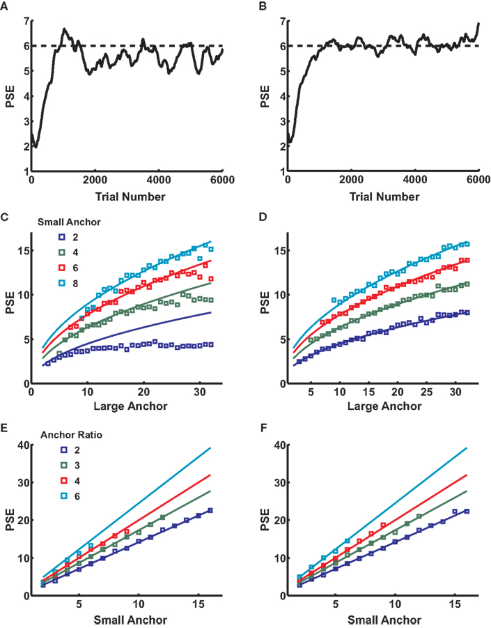
Figure 4. A simple learning algorithm reproduces location of the PSE. (A) A sample learning curve for the first 6000 trials of a bisection block with anchors 3 and 12. Dotted line marks the theoretical value of 6. Value learned by the algorithm with linear-hyperbolic inputs is around 5.3. (B) Same as (A) for the logarithmic model. Note that the mean PSE value is now equal to the geometric mean of the anchors. (C) PSE as a function of large anchor value for a series of small anchor values (different colors). Lines represent theoretical predictions based on the geometric mean formula. All series show increasing departures from Weber’s Law behavior at high numerosities, particularly for small anchor value 2. (D) Same as (C) for the logarithmic model. (E) PSE as a function of small anchor value for fixed ratios of large to small anchor values (different colors). Simulated data are roughly in line with linear predictions based on the geometric mean formula over the range tested. (F) Same as (E) for the logarithmic model.
Our model of numerosity encoding in the bisection paradigm takes as its starting point the measured monotonic response functions and spiking statistics of neurons in LIP. Though these neurons conform to neither the linear/scalar variance nor logarithmic/constant variance models of graded numerosity encoding previously proposed, we are able, using a simple decision rule in conjunction with a hypothesized bias input, to reproduce observed bisection behavior. In addition, we are able to predict adherence to Weber’s Law over a significant range of anchor value pairs. However, the differences between our model and previous proposals are illuminating, and offer predictions for future experiments. In the case of our linear/hyperbolic model (again, to be distinguished from the logarithmically widening preferred-numerosity responses in population coding models), we predict gradual deviations from Weber’s Law behavior at very large numerosities, corresponding to PSEs of 10 or more. In our logarithmic model, we expect to see increasing nonlinearity in neuronal responses for very large numerosities, though we do not expect increasing Poisson noise to disrupt the Weber’s Law property (see Supplementary Material). In both cases, we expect a constant relative shift in firing rates between the response curves for different pairs of task anchor values (and thus different PSEs), a key prediction of the model testable in future experiments.
In addition, we hypothesize that the disparity between measured task performance in animals and the classification behavior of an ideal observer using our neuronal data is due, at least in part, to additional noise added in the response selection process. We argue that this noise, which often results in choices the animal should “know” are wrong, is needed by the reinforcement learning algorithm that learns the task’s reward contingencies and the location of the PSE. Because greater sampling from both options leads to better estimates of each option’s value, less accurate choice behavior, paradoxically, leads to grater optimality in choosing the location of the PSE that results in maximum reward. Indeed, we conjecture that this need for flexible learning algorithms may explain similar discrepancies between ideal-observer and measured animal behavior in other classification tasks (Shadlen and Newsome, 2001
). Finally, our algorithm is noteworthy in that it makes no use of “right” or “wrong” classification behavior, nor requires explicit knowledge of the underlying classification rule. Choosers simply learn the average value of responses in the presence of stimuli, and update the internal model accordingly. As a result, task performance may be viewed through the lens of reward maximization, and our algorithm makes predictions for cases in which responses are differentially or probabilistically rewarded.
The Supplementary Material for this article can be found online at http://www.frontiersin.org/behavioralneuroscience/paper/10.3389/neuro.08/001.2010/
The authors declare that the research was conducted in the absence of any commercial or financial relationships that could be construed as a potential conflict of interest.
Green, D., and Swets, J. (1989). Signal Detection Theory and Psychophysics. Peninsula Publishing. Available at: http://www.amazon.com/Signal-Detection-Theory-Psychophysics-Marvin/dp/0932146236/ref=sr_1_1?ie=UTF8&s=books&qid=1263939907&sr=8-1
.