Different methods to define utility functions yield similar results but engage different neural processes
1
Department of Neurology, University of Magdeburg, Germany
2
Faculty of Economics, Empirical Economics, University of Magdeburg, Magdeburg, Germany
3
Center for Behavioral Brain Science, Magdeburg, Germany
4
Department of Neuropsychology, University of Magdeburg, Magdeburg, Germany
Although the concept of utility is fundamental to many economic theories, up to now a generally accepted method determining a subject’s utility function is not available. We investigated two methods that are used in economic sciences for describing utility functions by using response-locked event-related potentials in order to assess their neural underpinnings. For determining the certainty equivalent, we used a lottery game with probabilities to win p = 0.5, for identifying the subjects’ utility functions directly a standard bisection task was applied. Although the lottery tasks’ payoffs were only hypothetical, a pronounced negativity was observed resembling the error related negativity (ERN) previously described in action monitoring research, but this occurred only for choices far away from the indifference point between money and lottery. By contrast, the bisection task failed to evoke an remarkable ERN irrespective of the responses’ correctness. Based on these findings we are reasoning that only decisions made in the lottery task achieved a level of subjective relevance that activates cognitive-emotional monitoring. In terms of economic sciences, our findings support the view that the bisection method is unaffected by any kind of probability valuation or other parameters related to risk and in combination with the lottery task can, therefore, be used to differentiate between payoff and probability valuation.
The concept of utility functions is fundamental to economics. Utility features prominent in most economic theories, as it is not a good’s quantity or money per se that determines the actions of human beings, so called agents, but the utility they obtain from the good. Equilibrium concepts like the Nash equilibrium for strategic interactions of agents, the Walrasian equilibrium of economies, financial theory or the theory of political decision making are based on utility considerations. Expected utility theory and its modifications like Prospect Theory (Kahneman and Tversky, 1979
) are the most established theories for decision making under risk. Utility theory is well-founded by an axiomatic approach with few intuitive axioms. In contrast to its theoretical importance, a generally accepted procedure how to measure utility does not yet exist. The need to have a method for determining utility functions is obvious, since violations of expected utility theory are frequent, in particular in the area of risky decision making. Without a generally accepted approach for identifying utility, it is impossible to figure out which theoretical predictions made by utility function related models do not fit observed decision making processes and hence many predictions of economic models are neither testable nor implementable. Several key questions have therefore be answered: Is the concept of utility functions a normative construct, does it capture the key features of decision making processes or is it just a tool for describing behavioral data?
In the present paper we focus on the utility of money. Two main methods to determine the utility of money are discussed in the literature: the evaluation of lotteries and the bisection method.
In the first approach, certainty equivalents (CE) of lotteries are determined for various amounts of money and various probabilities. Payoffs which are either 0 or x1 (x1 = 100 in Figure 1
A) are offered by a lottery with a chance to win p = 0.5 or a sure win (“C” in Figure 1
A) with the participant’s task to choose one option (lottery or sure win). The CE is represented by the sure payoff for which a subject is indifferent between the two alternatives. Within this framework a utility function is determined based on its assumed functional form, a probability weighting and an econometric analysis. A key problem for econometric analyses is that each model, e.g. Regret Theory (Loomes and Sugden, 1982
), Prospect Theory (Kahneman and Tversky, 1979
), or Disappointment Theory (Bell, 1985
), assumes a distinct functional form for the evaluation of money and probabilities. Consequently, the determination of utility functions for risky decisions differs across theoretical approaches. Another shortcoming of the binary lottery approach is that the evaluation of probabilities and money are not fully separable. Thus, risk aversion can be attributed either to the shape of the utility function or to the probability weighting. The statement of Prospect Theory that individuals are risk averse for positive payoffs or high probabilities therefore depends crucially on the assumptions of econometric analysis. On the other hand, one of this method’s advantages is that agents really decide between options which lead to payoffs.
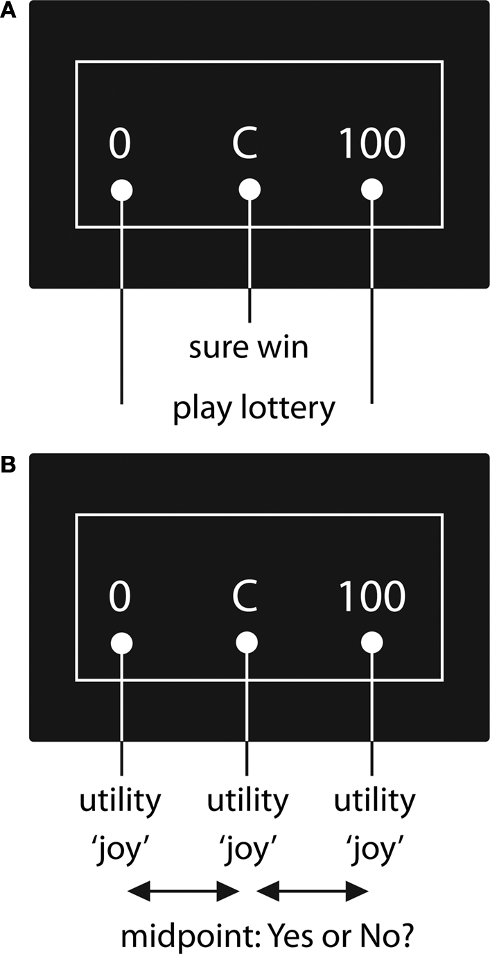
Figure 1. Prototypical decision task for the binary lottery (A) and the bisection task (B).
In the second approach, the bisection method, agents are asked to specify differences in the utility associated with monetary payoffs. In this method, a utility function is elicited by determining mean points of utility between two utility values, which are x1 and 0 in Figure 1
. One possibility is, to present agents with two amounts of money, x1 and 0, and ask them which amount of money M divides the utility difference u(x1) −u(0) into halves, i.e. u(M) = (u(x1) + u(0))/2 = u(x1)/2. It is also feasible to show a third amount of money x3 (“C” in Figure 1
) and to ask if this value divides the difference of x1 and 0 into halves [(u(x1) + u(0))/2 = u(M)]. To achieve a monetary valuation without using lotteries, subjects are asked to evaluate their perceived “happiness that money brings” (Galanter, 1962
). In the present study the term “joy” is used (associated with receiving a specified amount of money) in order to induce a monetary valuation context. By varying the parameters, a utility function can be obtained. This method’s advantage is that the resulting utility function does not depend on probabilities and the specification of a functional form, meaning that no theoretical presumptions are required. Its disadvantage is that decisions are neither connected to monetary nor to hypothetical payoffs.
Both methods have been widely used and discussed in the literature. In most studies in experimental economics the evaluation of lotteries is used to determine utility functions or to test theories. The key argument for preferring the lottery method over the bisection method is that economic decisions should involve monetary payoffs, otherwise the decisions “are not for real”. Figure 2
illustrates the theoretical foundation for both procedures. By asking for the CE or the midpoint the value on the x-axis is determined, i.e. CE or M, respectively. The value u(CE) or u(M) on the y-axis is not given. For the bisection task it is by definition half of the utility of x1. In the lottery condition this value depends on the theory describing the evaluation of lotteries. In Prospect Theory for example it is Π(0.5)*u(x1). If the probability weight Π(0.5) is small enough one might also obtain a linear utility function even if the CE is below the expected value. Therefore one has to know Π(0.5) if one wants to determine the utility function by means of the lottery method. Assuming that both methods are based on the same utility function one could combine both methods to first get the utility function by means of the bisection method and then determine the probability weight of 0.5. This procedure can also be applied to probabilities different from 0.5, enabling one to determine a probability weighting function, and a utility function experimentally by combining both methods.
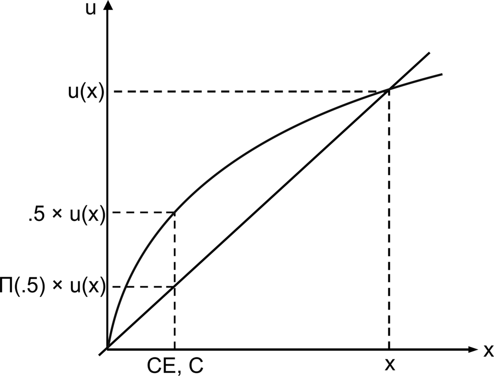
Figure 2. Theoretical procedure how to determine a utility function if probabilities are perceived linearly.
While economic scientists have pointed out differences between the two methods, e.g. stating that decisions in the bisection task are not for real, such difference might better be captured from a cognitive neuroscience point of view. Moreover, a cognitive neuroscience approach to this problem may also reveal differences in the neural processes involved in the two decision methods. In human beings decision making processes are supervised “online” by cognitive control mechanisms enabling adaptive behavior in a most flexible manner (Ridderinkhof et al., 2004
; Botvinick, 2007
). Typical simple situations in which these mechanisms have been studied involve response selection from several action alternatives or the evaluation of currently made decisions. By using event-related potentials (ERP) the neural underpinnings of these control mechanisms can be revealed. One ERP component related to response evaluation processes is the error-related negativity (error related negativity (ERN) Falkenstein et al., 1991
; Gehring et al., 1993
). This component was initially described to appear 50 to 100 ms following an incorrect response in choice-reaction tasks at fronto-central electrode sites and was postulated to reflect the perceived discrepancy between the intended and the actually performed action. Source analysis as well as simultaneous analysis (Dehaene et al., 1994
) of ERPs and functional magnetic resonance imaging (fMRI,Mathalon et al., 2003
; Debener et al., 2006
) have shown that the ERN is generated in the anterior cingulate cortex, an area that is closely linked to several cognitive control mechanisms involved in decision making (Gehring and Knight, 2000
; Paus, 2001
) and in the processing of risk related feedback information (Yeung and Sanfey, 2004
; Cohen et al., 2007
). Recent investigations have shown that the ERN is also sensitive to characteristics in error processing that are not directly linked to the violation of objective criteria. For example, an error may be more relevant by associating it with the loss of money (Hajcak et al., 2005
) or by manipulating the participant’s mood state (Tucker et al., 1999
; Luu et al., 2000
; Wiswede et al., 2009
). These manipulations also influence ERN amplitudes. As Hewig et al. (2007)
have shown, the high risk choices resulted also in an ERN, because such a selection implies a high chance not to get the response’s intended outcome and will be processed as an error-like deviation from advantageous choice strategies. Based on their initial approach explaining error processing in terms of reinforcement learning (Holroyd and Coles, 2002
; see also Munte et al., 2007
for electrophysiological evidences) Holroyd and Coles (2008)
described the occurrence of an ERN in the absence of external ascertainable response criteria. Accordingly, responses are matched against internal criteria that were formed by individual learning histories and ERN amplitude is driven by the internal classification of a given response as “sub-optimal” (Holroyd and Coles, 2008
). The ERN thus may reflect the subjective value of a potential response.
In the present investigation we use the ERN as a tool to characterize the neural implementation of decisions made in the lottery and bisection paradigms. Our prediction is that lottery decisions will be associated with increased monitoring, since the payoff instruction increases the subjective relevance or value in this task which should amplify the ERN amplitude. ERPs in the bisection task should not feature an ERN, because here responses have neither to be matched against set criteria nor are they associated with subjective relevance. Thus, we assume that fundamentally different neural processes will be engaged by the two methods. Importantly, we further ask whether the engagement of such different neural processes would also lead to differences in the estimates for the utility function of money.
Participants
Sixteen neurological healthy, right-handed participants gave informed consent to take part in the study (10 women, age range 21–29). Two of these were excluded because of technical problems and one participant made no disadvantageous responses in the range from 390 to 100 and was excluded from data analysis as well. The final data-set thus comprised 13 participants. They were paid €7 per hour. The study protocol had been approved by the ethics committee of Magdeburg University.
General Procedure
Participants were seated in a comfortable chair in front of a 19″-CRT monitor. A modified computer mouse was positioned under each index finger as a response device. The experiment consisted of two sessions which took place within 3–7 days. In both sessions identical stimulus material was presented but with differing task instructions. Every session began with 20 practice trials to familiarize subjects with the task. Thereafter the session started comprising 10 blocks of 82 trials each.
Task
In each trial, lasting between 2700 to 3400 ms, a string of three numbers surrounded by a white box was presented (see Figure 3
). The two outer numbers were shown first. After 1000 ms, the inner number was added and the completed array stayed on the screen for another 1000 ms. The array’s left number was always zero. If numbers on the right were between 800 and 1000, the mid position numbers varied between 100 and 700, in case the right-sided numbers were between 1020 and 1200, mid position numbers were in the range of 300 to 900. Numbers in the middle were varied in steps of 50, right-sided numbers in steps of 20. Before presentation numbers within each string were multiplied by 1, 10 or 100, resulting in three classes of strings (e.g. “0 350 1120”, “0 3500 11200” and “0 35000 112000”).
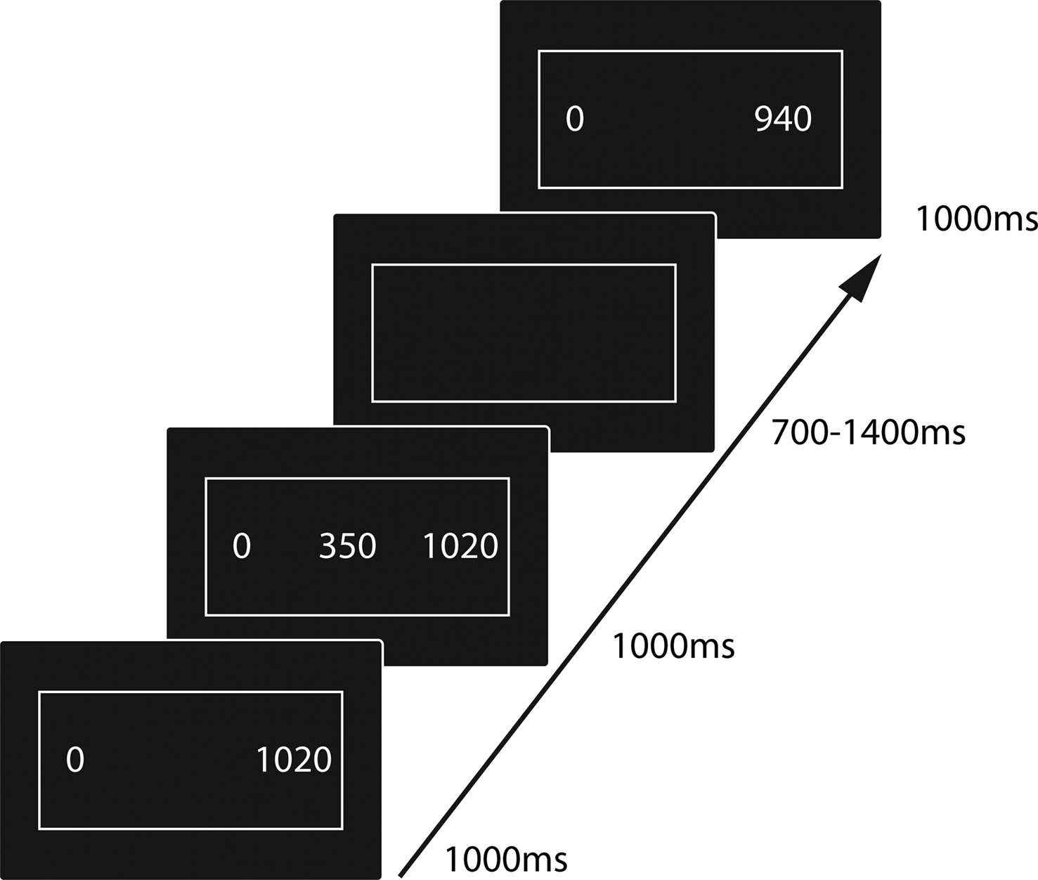
Figure 3. Experimental paradigm.
In the binary lottery task participants had to choose to either get the amount of money corresponding to the center number or to play a lottery in which the outer numbers were the lottery’s stakes played out at a fifty-fifty chance. Participants were explicitly told that the lottery game was hypothetical only; to that effect subjects expected no real payoff. They indicated their choices by pressing a button with the left or right index finger.
In the bisection task, the outer numbers corresponded to the utility interval’s boundaries and the inner number to this interval’s center. To keep the emotional framing of the bisection task comparable to the lottery task participants were instructed to imagine for each presented number the joy they would feel when getting this amount of money in Euro. By pressing the left or right index finger (YES/NO) subjects indicated whether the difference in perceived joy between the left – this number is always zero- and the center number and the center and the right number was felt to be equal (YES) or not (NO, see Figure 1
). In both conditions subjects did not receive any performance feedback.
EEG-Recording and Analysis
The electroencephalogram was recorded from 28 tin electrodes, referenced against an electrode place on the left mastoid process, mounted in an elastic cap and placed according to the international 10–20 system. EEG was re-referenced offline to the mean activity at the left and right mastoid processes. All channels were amplified (bandpass 0.05–30 Hz) and digitized with 4 ms resolution. To control for eye movement artifacts, horizontal and vertical electrooculograms were recorded using bipolar montages. To eliminate eye movement contamination from EEG signals we used second order blind source separation as described by Joyce et al. (2004
; for a comparison to other methods see Kierkels et al., 2006
). Additionally, we controlled for other artifacts, e.g. muscle or heart rate, by visual inspection and removed afflicted epochs if necessary.
The generation of bins for ERP analysis was based on a difference value calculated for each trail. This difference value was computed by subtracting the arithmetic middle of the two outer numbers from the number presented in the center of the array. To give an example the numbers shown in Figure 3
are used: The outer numbers of the array are 0 and 1020, the number in the center is 350. The arithmetic middle of the two outer numbers is (0 + 1020)/2 = 510 and the resulting difference is 350 − 510 = −160. The negative value of this difference indicates that the number presented in the array’s center is smaller than the arithmetic middle of the corresponding outer numbers. Accordingly, numbers presented in the array’s center larger than the arithmetic middle of the outer numbers produce a positive difference value. Based on the difference values we sorted trials into five bins including the differences 390 to 100, 90 to 50, 40 to −40, −50 to −90 and −100 to −400. For each of these bins, we computed response-locked averages with an epoch-length of 900 ms (baseline −300 to 0) separately for “yes” and “no” responses. For each subject, averages were filtered using a 1–8 Hz band pass filter before calculating the mean amplitude 30–70 ms after response for statistical analysis. This time-window has been shown to capture the ERN component which typically has a maximum around 50 ms. To test for effects, we calculated an ANOVA with the factors condition (lottery/center judgement), response (yes/no, where “yes” in the lottery condition is related to choosing money and “no” choosing the lottery) and bin (five bins) for the electrode site Cz. Significance values will be reported Greenhouse-Geisser corrected, but the degrees of freedom uncorrected. In order to identify conditions causing significant interactions or main effects the corresponding post-hoc t-tests were performed. To adjust the significance level of one-tailed post-hoc t-tests for multiple comparisons α was set to 0.05 and an improved Bonferroni procedure based on the ordered p-values was applied (Simes, 1986
). According to Simes (1986)
, let p(1) ≤ p(2) ≤ … ≤ p(j) be the ordered p-values for testing H0 = {H1,H2,..,Hi}. H0 will be rejected, whenever pi < i*α/j for i = 1, …, j (see also Samuel-Cahn, 1996
; Sen, 1999
for a critical discussion and Wendt et al., 2007
for its application on EEG data). According to this procedure we grouped our post-hoc-testing into two sets: comparisons for decisions at the indifference point [bin (−40; 40)] and comparisons for decisions made at the endpoint [bins (−400; −100) and (100; 390)]. Correspondingly, we calculated critical p-values for 6 and 7 post-hoc comparisons. A similar correction was applied to the 5 post-hoc tests of the behavioral data. The resulting critical values are shown in Tables 1 and 2
respectively.
Behavioral Analysis
We calculated the means μbisection, μlottery and standard deviations σbisection, σlottery for the bisection method and the lottery method respectively. For the Yes-responses of both methods we determined histograms that are representing the best fit to a normal or to a cumulative normal distribution function. For these histograms we calculated means and standard deviations. We tested if the bisection method’s mean μbisection can be the mean of the distribution (histogram) of the data under the lottery condition and if the lottery task’s mean μlottery can be the mean of the distribution under the bisection condition.
In a second analysis the same bins as used for the EEG analysis were assessed. Response frequencies were calculated for every participant by computing the percentage of ‘yes’ and ‘no’ responses given to each class of difference values. For statistical analysis the mean percentage values of ‘yes’ response were used only, since percentage values of both response categories are inversely related. For global effect testing, we performed a repeated measures ANOVA with the factors condition (lottery/center judgement) and bin (five bins, see previous section for details). Significance values will be reported Greenhouse-Geisser corrected, but the degrees of freedom uncorrected. For correction of post-hoc test’s alpha value see section “EEG-Recording and Analysis”.
Behavior
Choices made for each class of difference value (in mean percentage) are depicted for the lottery and bisection tasks in Figures 4
A,B respectively. We fitted a normally distributed density function for the data in Figure 4
A and a normally distributed cumulative distribution function for the data in Figure 4
B. This procedure results in μbisection = −14.33 and σbisection = 175.74 for the bisection method and μlottery = −32.57 and σlottery = 191.97 for the binary lottery method. In a t-test the Null hypothesis that μbisection = −32.57 is not rejected on the 40% level (absolute t-values are smaller than 0.64). The same holds for the Null hypothesis μlottery = −14.33. We observed a slightly concave utility function under both conditions (μ < 0) which corresponds to risk aversion in the lottery condition. The average μ is smaller in the lottery condition, but the difference is not significant.
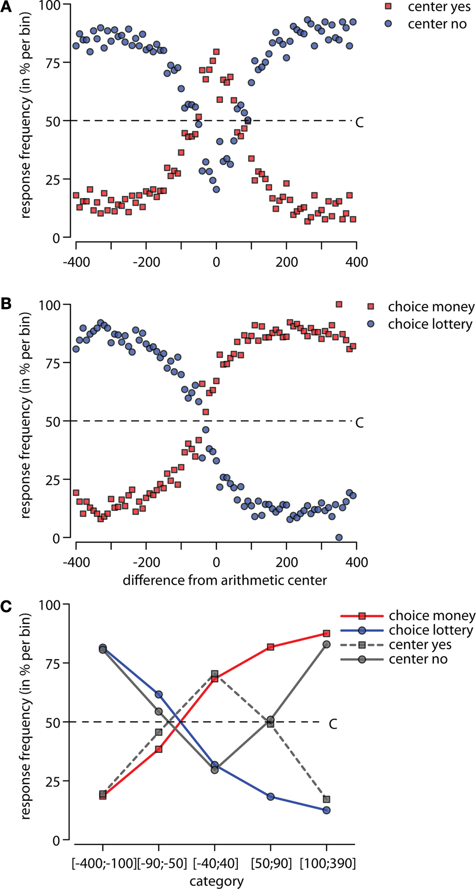
Figure 4. Behavioral data. Mean percentage of choices are shown for the binary lottery (A) and the bisection task (B). The center is indicated by a dashed line and refers to the indifference point in the bisection task. (C) depicts the cumulated choices per bin for both task. Circles referring to “YES”-, squares to “NO”-responses. Indifference point is indicated by a dotted line. Please note, that statistical comparisons were only calculated for YES responses.
Collapsing choices into 5 bins as done for the EEG analysis clearly illustrates the differences between the tasks (see Figure 4
C). Statistical analysis for the YES-responses reveals a significant interaction condition by bin (F(4,48) = 33.38, p < 0.001) as well as significant main effects (condition F(1,12) = 14.39, p = 0.003; bin F(4,48) = 32.04, p < 0.001). Comparing bins between conditions post-hoc contrasts are significant for the bins [100; 390] and [50; 90], but not for the remaining bins [−40; 40], [50; 90] and [100; 400]. For example, these tests show that the difference in the means of the CE and the mean point are not significant.
Event-Related Potentials
The response-locked grand average ERPs are illustrated in Figure 5
. A clear negativity with a peak latency at approximately 50 ms and a mediofrontal distribution (see Figure 6
) akin the ERN component emerged in the lottery task for those responses which entailed a divergence from the optimal behavior [i.e. choosing the lottery in bin (100; 390) and choosing money for bin (−100; −400)]. By contrast, obviously incorrect responses to the same bins in the bisection task (Figure 5
D, “center yes” responses in the bins [−100; −400] and [100; 390]) resulted in much smaller negativities. The amplitude of these negativities was similar to the responses in the indifference range (Figure 5
C). Statistical analysis of response-locked ERPs resulted in significant interactions condition × response × bin [F(4,48) = 7.18, p = 0.002], condition × response [F(1,12) = 5.29, p = 0.03], condition × bin [F(4,48) = 3.23, p = 0.03] and response × bin [F(4,48) = 3.91, p = 0.03]. With regard to main effects, only the ‘condition’ factor became significant [F(1,12) = 5.78, p = 0.03; for the remaining main effects response and bin F < 0.9, p > 0.4]. Post-hoc comparisons contrasting decisions between bins within and between conditions are illustrated in Table 2
.
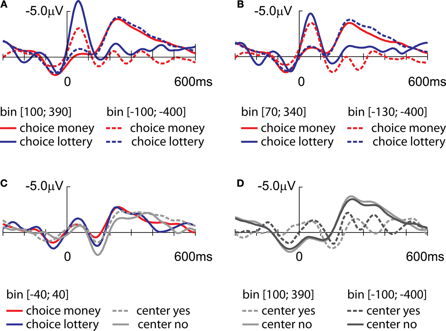
Figure 5. Response-locked event related potentials for the lottery’s task endpoints (A), the bisection’s task endpoint (C) and the indifference point for all conditions (D) at Cz are shown. (B) Depicts the lottery’s task ERPs which are corresponding to the bins equidistant to the indifference point [bin 70;340] and choice money [−130;−400].
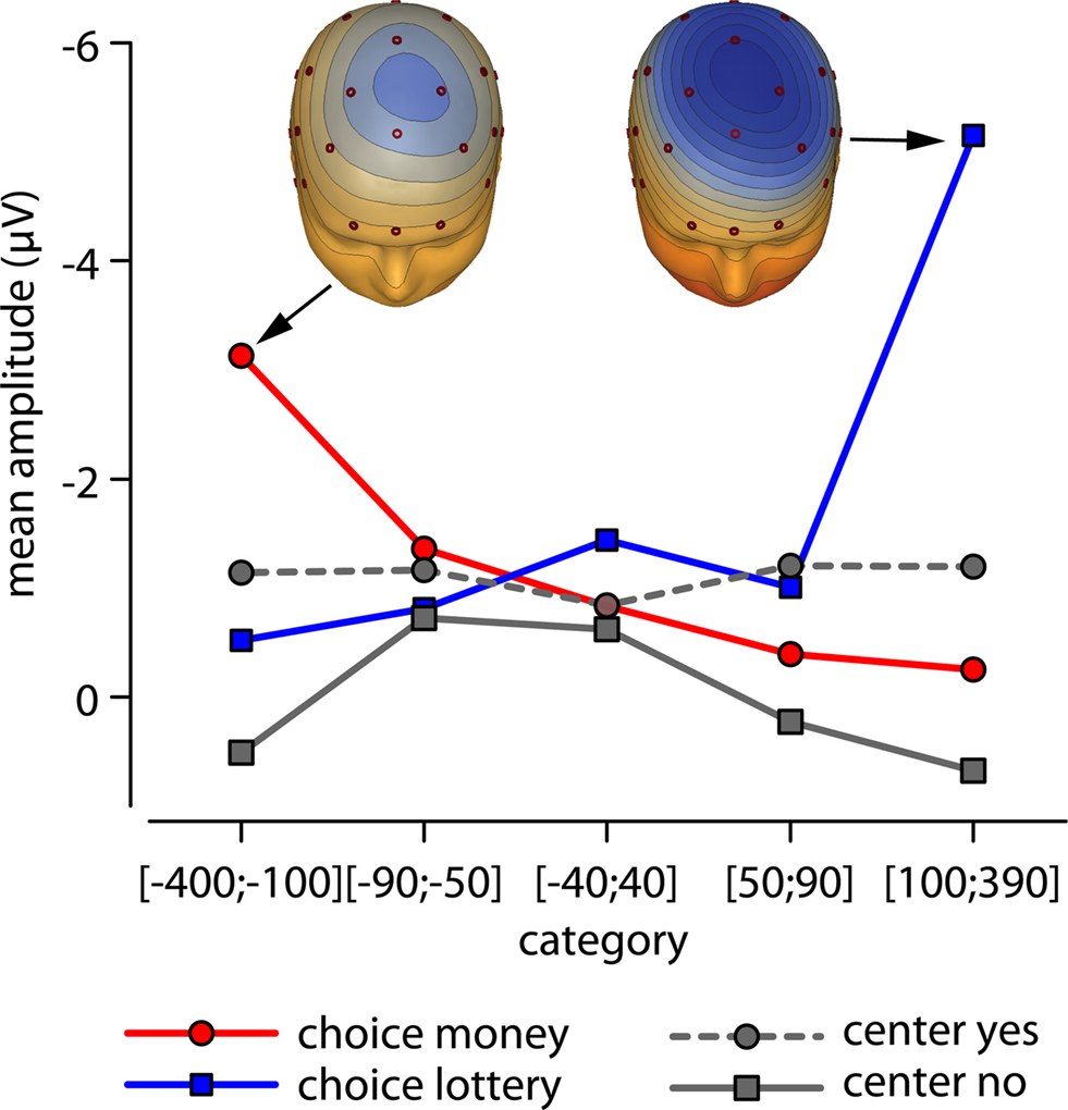
Figure 6. ERN topography. Topographies for the lottery conditions left) choice money [−100; −400] and right) choice lottery [bin 100; 390] are shown. The line graph depicts the mean amplitudes of the response-locked ERPs at CZ per category. Circles referring to “YES”-, squares to “NO”-responses.
Additionally, we checked whether differences in the ERPs seen between the unfavorable choices in the lottery task might simply be due to a different distance between the indifference point at −30 (see Figure 4
A) and the respective bins [100;390] and [−100; −400]. Therefore, two new bins were obtained according to the procedure described in section “EEG-Recording and Analysis”, but with new intervals (see Figure 5
B), which are equally distant from the indifference point. Compared to the original bins the ERN amplitude related to the unfavorable lottery choices decreases while the ERN for unfavorable money choices increases. Nevertheless, the difference between both conditions remains significant (one-tailed t-test, t = −2.08, df = 12, p = 0.03).
In the present study, action monitoring processes as indexed by the ERN component were differentially engaged in two decision making paradigms that have been frequently used in economic sciences to determine the utility of money. This suggests fundamental differences between the lottery and bisection methods at the cognitive and neural level. More specifically, in the binary lottery task a pronounced ERN characterized decisions in favor of the less advantageous options at either endpoint of the range of possible decisions. That is, an ERN was found for “lottery”-decisions in trials that would have yielded a sure win greater than the mean outcome of the lottery. Similarly, an ERN was present for “sure win”-decisions in trials in which the mean outcome of the lottery would have exceeded the sure win. The occurrence of an ERN in the lottery task can be interpreted as evidence for the subjects’ motivational participation even though the lottery’s payoffs were only hypothetical, as it is known from previous research that the appearance of an ERN depends on the subjective significance in a given task (Hajcak et al., 2005
; Holroyd and Coles, 2008
). The difference between the trial bins associated with the two most prominent ERNs indicates different degrees in action monitoring and is likely caused by the interaction of two factors: the difference between expected value and sure payoff on the one hand and the risk to sustain a potential loss on the other. For both kinds of decisions associated with an ERN the difference between the expected value of the lottery and the sure win was similar. Nevertheless, the ERN’s amplitude was larger for disadvantageous lottery decisions compared to the disadvantageous selection of a sure payoff. This suggests that the anticipation of a risky decision’s potentially negative outcome, namely to win nothing instead of getting a small but sure payoff in the unfavorable sure win selection, leads to increased activation of monitoring mechanisms despite similar expected values. One might argue, that this difference is simply caused by the dissimilar distances between the indifference point at −30 and the end-bins respectively (see Figure 4
B). However, the described effect persists (albeit somewhat smaller) even when trials were rearranged to yield bins that are equidistant to the indifference point. The change in ERN amplitude for these rearranged bins is due to the fact that, for lottery choices, the bin [70; 340] comprises less disadvantageous selections, whereas in the bin [−130; −400] the proportion of unfavorable choices increases. It is to be expected that the corresponding ERN amplitudes decrease and increase, respectively.
In contrast to the binary lottery task the bisection task’s incorrect responses at the end-bins are associated with a very small negative deflection, i.e. a rudimentary ERN. Although the amplitudes of these negativities are significantly different from the end-bins’ correct choices, the parameter values are indicating a much smaller degree of action monitoring involvement (Nieuwenhuis et al., 2001
; Burle et al., 2008
; Heldmann et al., 2008
) and are similar to the amplitudes observed for the indifference point. Based on our previous argumentation the rudimentary ERNs can be seen as an indicator for the absence of risk perception in these conditions.
In which way are the ERP results able to inform economic reasoning? Looking at the economic starting point of our analysis shown in Figure 1
we discussed the differences and similarities between the bisection and the binary lottery method. The bisection method determines the mean point in utility between the two monetary amounts only by the utility function of money with the following formula: u(M) = 0.5*u(x1). In the binary lottery method the CE is determined by the utility function of money and other factors connected with the risk of the lottery, like probability weighting in Prospect Theory. According to Prospect Theory the CE is: u(CE) = Π(0.5)*u(x1). The difference between both formulas is obvious: the weighting of probabilities Π(prob). Using the formula of Prospect Theory we would expect the CE and the mean point in the bisection task M to be equal if we assume Π(0.5) = 0.5. Here, only the utility function of money determines the CE.
In our investigation behavioral as well as ERP data suggest that both methods used are resulting in similar utility functions for money. Although there are visible differences between the bisection and the binary lottery task’s indifference point, indicating risk avoidance, the statistical analyses revealed that these differences are absolutely not significant. The corresponding ERPs for decisions around the indifference point of the bisection and the lottery task (see Figure 5
C) are also indicating, that action monitoring processes are not differentially engaged in the related decision making processes. Postulating the bisection method captures utility of money itself and, as argued previously, the binary lottery the combination of utility and risk, an implication of our finding is that utility function and probability weighting can be separated by initially determining the utility function with the bisection method and afterwards using the obtained function as input in the lottery method to get the lottery’s probability weighting experimentally. This procedure could also be applied to lotteries with probabilities different from 0.5 and would allow for a more precise discrimination between effects of the probability weighting and utility function for money. The same procedure allows for the separation of other effects related to risk and not to money evaluation as well. For example, the implications of Regret or Disappointment Theory can be tested more easily by a combination of these two methods, since the result of the determination of the utility function can be used in the analysis of the lottery method. In general, using both methods and looking at the differences helps to characterize situations connected with risk (money and probabilities) in comparison to situations connected with certainty (money only).
It is important to note that ERNs were observed in the lottery condition even though money was not paid. As we stated previously, this indicates that despite the absence of real payoffs the choices made in the lottery task were subjectively more engaging compared to the bisection task and impelled participants to control their behavior to a larger extend. Assuming that hypothetical payoffs are less engaging then real payoffs, one would expect an increase in subjective relevance for real payoffs and therefore increasing ERN amplitudes. In line with the argumentation by Hewig et al. (2007)
subjective relevance of an intended behavioral outcome is one factor that drives sensitivity for risk related choices. Therefore, we believe that it is justified to ascribe the hypothesized ERN amplitude increase for lotteries with real payoffs partially to an altered perception of risk.
According to standard economic theory of risky decision making the choice of an individual is solely determined by consequences and probabilities entailed in a decision. The influence of time between the presentation of the problem, the decision and the realisation of the outcome is very often neglected. In the present study we showed that the temporal resolution of the ERP method and its ability to reveal cognitive processes that are not directly linked to perceivable behavior make it possible to identify the point in time at which post-decision evaluation processes takes place. That is, if the performed choice fits the subject’s response strategies and finally their long-term goals (Albers et al., 2000
).
In summary, we have shown that the combination of the bisection and the binary lottery task allows to separate probability weighting and the perception of risk in the determination of utility functions for money. We characterized common properties and differences of these two methods. Our ERP results are also indicating, that disadvantageous choices in the risky decision making task are processed differentially by cognitive action monitoring processes. Since we found no evidence for differences around the indifference point at the behavioral or the neural level the use of both methods to determine the utility of money will result under the given conditions in similar estimates.
The authors declare that the research was conducted in the absence of any commercial or financial relationships that could be construed as a potential conflict of interest.
This work was supported by the DFG (SFB 779 projects A3 and A5) awarded to Thomas F. Münte and Hans-Jochen Heinze. Also supported by a special grant of the Center for Behavioral Brain Sciences, Magdeburg, to Marcus Heldmann.