The effects of background noise on the neural responses to natural sounds in cat primary auditory cortex

Introduction

Whereas the representation of simple stimuli such as pure tones or amplitude- or frequency-modulated sounds in primary auditory cortex (A1) of mammals has been described in great detail (Bizley et al., 2005 ; Joris et al., 2004 ; Kadia and Wang, 2003 ; Liang et al., 2002 ; Moshitch et al., 2006 ; Nelken and Versnel, 2000 ; Read et al., 2002 ; Ricketts et al., 1998 ; Sutter and Loftus, 2003 ; Tan et al., 2004 ; Tian and Rauschecker, 1998 ; Tomita et al., 2004 ; Wehr and Zador, 2003 ), the processing of complex sounds, in particular natural sounds, in A1 is not well understood. Studies that have used natural sounds have shown that neurons in A1 are exquisitely sensitive to the detailed structure of complex sounds. In particular, one consistent finding (Creutzfeldt et al., 1980 ; Gehr et al., 2000 ; Machens et al., 2004 ; Pelleg-Toiba and Wollberg, 1991 ; Rotman et al., 2001 ; Sovijarvi, 1975 ; Wang et al., 1995 ) is that although the best frequency (BF) and the frequency response area (FRA) of a neuron are important determinants of its responses to a sound, individual neurons may respond idiosyncratically to different sounds.

Thus, in the awake squirrel monkey, Pelleg-Toiba and Wollberg (1991) found that only in 2%of the neurons the responses to species-specific calls and time reversed calls (“llacs”) were mirror image of each other, and only in 34%of the neurons at least one call elicited a response that corresponded to the temporal modulation of the acoustic waveform. Although they concluded that complex calls are represented by neuronal populations distributed throughout cochleotopic space (and not by call detectors), the responses of many neurons were not simply related to the acoustic features of the calls.

A number of studies reached the conclusion that responses of neurons in auditory cortex show significant non-linearities. For example, recently Machens et al. (2004) recorded responses to natural sounds intracellularly in the auditory cortex of anesthetized rats. They estimated spectro-temporal receptive fields, and concluded that this dynamic linear representation accounted for only 11%of the variability of the responses. Furthermore, using simple non-linearities such as adaptation, threshold, and saturation did not improve the fit by much. Using artificial stimuli, Sahani and Linden (2003) showed also a substantial amount of non-linearity in the responses of auditory cortex neurons in anesthetized mice and rats.

In order to study the responses to natural sounds in a reasonably controlled situation, we extracted a small set of bird chirps that consisted of a frequency- and amplitude-modulated tones from natural recordings (Bar-Yosef et al., 2002 ). These bird chirps are essentially frequency- and amplitude-modulated tones, and are therefore similar to the artificial sounds often used in auditory studies. The chirps were first presented within their original temporal context (250 ms of sound preceding and following the chirp), and were then successively simplified: first a short segment containing only the chirp was extracted from the longer segment; then background noise was removed, leaving only the modulated tone; and finally this cleaned call was replaced by an artificial sound that had a similar frequency trajectory but no amplitude modulation. All simplification steps were associated with substantial changes in the responses. We argued that such spectro-temporal context-dependence could play an important role in accounting for the difficulties encountered in attempts to relate the responses of A1 neurons to simple and complex sounds. In particular, the complexity of auditory cortical responses seems to be due both for complex temporal interactions (as demonstrated by the differences in responses to the same chirp embedded within its original temporal context and the chirp presented by itself) and to simultaneous interactions between the main acoustic components of a sound (the bird chirp in this case) and the simultaneously present background noise.

In the present paper, we study specifically the simultaneous interactions between chirps and background noise, since the background noise was weaker than the main chirp by 13 dB on average. To study these interactions in detail, the natural stimuli used by Bar-Yosef et al. (2002) were separated here into the dominant chirp, its presumed echoes and a wideband background noise component. We studied the responses elicited by these acoustic components when presented alone and in combination. The main finding of this study is that in many neurons, the responses to the natural sounds appear to be evoked by the background components in spite of the presence of the acoustically dominant chirp within the neuronal FRA.

Materials and Methods

Single neurons were recorded in the A1 of halothane-anesthetized cats. Animal preparation, the electrophysiological techniques, and the acoustic stimulation are all described in a previous paper (Bar-Yosef et al., 2002 ). All procedures were approved by the animal use and care committee of the Hebrew University-Hadassah Medical School. Briefly, recordings were made using 2–4 glass-coated tungsten electrodes simultaneously. Sounds were generated either on-line or presented from pre-recorded files using a digital to analog converter (TDT DA3-4), attenuated (TDT PA4), and switched on and off using a linear, 10 ms ramp (TDT SW2). Tones and broadband noise stimuli (BBN) were presented at a sampling rate of 120 kHz. The natural sounds and their modifications were presented at their original sampling rate of 44.1 kHz. Anti-aliasing filtering followed analog conversion. The sounds were presented to the animal through a sealed, calibrated system (designed and built by Garry Sokolich).

Sound stimuli

The natural stimuli used in this study were described in detail in a previous paper (Bar-Yosef et al., 2002 ). All natural stimuli containing frequency-modulated tones were extracted from field recordings (©the Library of Natural Sounds, Cornell Laboratory of Ornithology, Ithaca, New York). A statistical analysis of all segments dominated by frequency-modulated tones was performed, and six representative natural stimuli were selected.

Each of the six stimuli (called Natural below, see Bar-Yosef et al., 2002 ) was separated into three basic components: The clean bird chirp (Main), its echo (Echo), and the wideband background noise (Background, shortened to “Back” in the figures). The Natural and Main versions are identical to the stimuli with the same names used in Bar-Yosef et al. (2002) . All seven combinations of the three basic components were used to test the neurons. Figure 1 illustrates all the stimuli used in this paper.

FIGURE 1

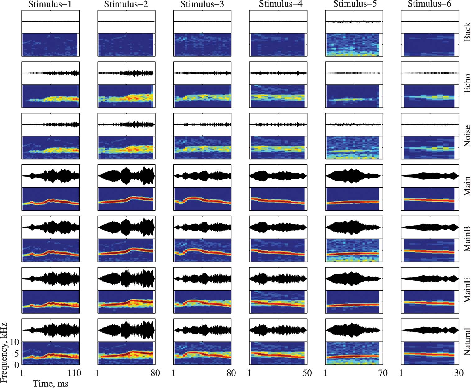
Figure 1. The bird song stimuli and their modifications. Each version is represented both as an oscillogram and as a spectrogram. The frequency range for all spectrograms is 0–10 kHz. All spectrograms share the same color scale (covering a range of 60 dB), and all the oscillograms share the same scale. The time scale is identical for all versions of the same stimulus (in columns). The versions and their relationships are (from bottom to top): Natural (Main + Echo + Background), Main + Echo, Main + Background, Main, Noise (Echo + Background), Echo, and Background.

Main was extracted from the full Natural stimulus in the following way: a fast Fourier transform (FFT) was computed on 256-point frames. It was used to locate the approximate center frequency of the bird chirp at that frame. The exact frequency of the peak of the (continuous frequency) Fourier transform was then located by maximizing the exactly interpolated FFT values:

where F(ω) is the continuous-frequency Fourier transform, N is the length of the FFT, and ω_k are the FFT frequencies. This formula gives the values of the discrete Fourier transform, evaluated at frequency ω, in terms of the Fourier transform computed at the FFT frequencies. The amplitude and phase of the Fourier transform at the peak frequency were used to generate one sample of the Main stimulus, corresponding in time to the center of the FFT frame. The FFT frame was shifted by one sample, and the procedure was repeated for each sample of the Natural sound. Next, the Main sound was subtracted sample by sample from the natural sound, leaving the noise components (referred to later as Noise). These consisted of a narrowband component occupying approximately the same spectral extent as the bird chirp, and a wideband component. The narrowband component had a characteristic temporal structure: it appeared at each frequency only after the same frequency occurred in the Main. Therefore, it is probable that the narrowband component consisted of echoes of the main chirp.

To separate these echoes from the other parts of the background noise, we first tried to model the echoes by a time-invariant FIR filter. This approach led to unsatisfactory results, probably due to atmospheric time-varying processes. Consequently, a heuristic approach was developed. First, artificial echo filters whose coefficients were random Gaussian numbers were created, mimicking random reverberation of the sound. These filters were used to create artificial echoes of the main chirp, and the length of the artificial echo filters was adjusted to obtain the best least-squares fit with the spectrogram of the Noise. Once the optimal length was found, spectrograms generated with 100 different artificial echo filters were averaged to create a “typical” echo pattern. Next, the artificial echo pattern was used to delimit the spectro-temporal region on the Noise spectrogram in which the real echo was likely to occur. This region corresponded satisfactorily with the extent of the narrowband component in the Noise as judged by visual inspection. Finally, each sample of the Noise was positioned at the center of a 256 FFT frame. The spectral components inside the presumed frequency range of the echo at that time period were attenuated to the background level, without changing their phases, and the central sample of the frame was re-synthesized. The resulting signal was used as an estimate of the Background. The echoes were separated from the rest of the background by subtracting Background from Noise, sample by sample.

Since the initial few milliseconds of a short sound may be crucial for determining neuronal responses in A1, it was necessary to ensure that Main is indeed the dominant acoustic component starting from sound onset. For that purpose, a detailed view of the onset of the three basic components, plotted on top of the appropriate Natural version (in gray), is presented in Figure 2 for all stimuli. Main dominated the sounds starting already at stimulus onset. For some stimuli, Echo was the second largest and Background the smallest of the three basic components during these initial 2 ms of the stimulus (e.g., Stimuli 2 and 4), although for other stimuli Background could be initially larger than Echo (e.g., Stimulus-5). On average, Echo was 13 dB weaker than Natural and Background was 29 dB weaker than Natural.

FIGURE 2

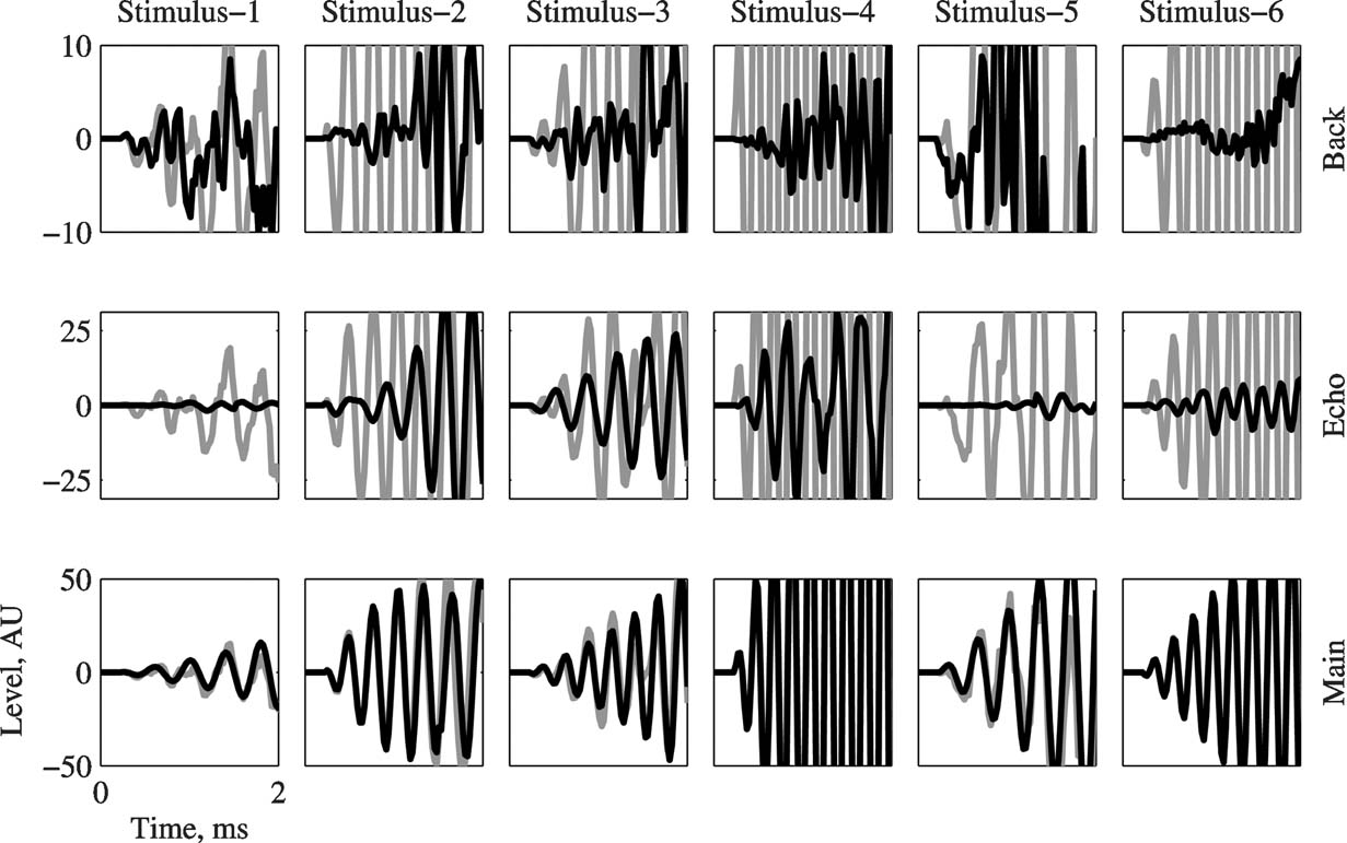
Figure 2. The initial 2 ms of Main, Echo, and Background (in black), overlaid on the corresponding waveform of Natural (in gray). The ordinate scales are given in A∕D units, and are different for each version. In all the cases, Main is the dominant component starting from stimulus onset.

Whereas the separation of Main from the Natural was rather easy and based on obvious criteria, the separation of Noise into Echo and Background was less satisfactory. For example, although the spectrogram of Background was rather flat, the phase structure inside the echo band was unaffected by the manipulation, and could be heard as a weak narrowband residue within the wideband noise. Nevertheless, the spectral structure and the subjective quality of Echo and Background were sufficiently different to use them profitably in the physiological experiments.

The three basic components (Main, Echo, and Background) were used to create three additional versions of the stimuli (Figure 1 ): Main + Echo, Main + Background, and Noise (Echo + Background). Thus, a total of seven versions of each of the six stimuli were used in the experiments (Natural, Main Echo, Main + Background, Main, Noise, Echo, and Background).

Seven of the neurons used in this report were collected during preliminary experiments, and were studied using a somewhat different set of stimuli. In these experiments, only three versions of each stimulus were used: Natural, Main, and Noise. Main was separated from Noise by estimating its center frequency and amplitude at each frame, but without using the exact phase. Thus, for these stimuli, Main could not be subtracted sample by sample from Natural to create Noise; instead, the relevant spectral components of Noise were attenuated by 17 ± 3 dB (depending on the stimulus). Comparing the responses of the two groups of neurons to the different sound stimuli did not reveal any clear differences. Therefore, they were pooled for analysis as one population.

Experimental protocol

The microelectrodes were inserted into the low-frequency area of A1 as described by Reale and Imig (1980) . Neuronal activity was identified on the basis of spontaneous activity or responses to tones and BBN. Each unit was characterized manually by determining approximately its BF and its threshold to BBN. Next, the preferred aurality was determined using BBN rate-level functions to the left (ipsilateral) ear alone, to the right (contralateral) ear alone, and to both ears diotically. The rest of the experimental paradigm was performed at the preferred aurality (ipsilaterally, contralaterally, or diotically). FRA was measured using a matrix of 45 frequencies logarithmically spaced from 100 to 40 000 Hz and 11 sound levels linearly spaced between 99 and 12 dB attenuation (corresponding to about 0–87 dB SPL). Finally, the natural stimuli and their modifications were presented twenty times each in a pseudorandom order. The attenuation was set at 20 dB above the neuron BBN threshold. At this setting, the level of the tonal component was typically 60–70 dB SPL. Presentation rate was always 1 second, both for the artificial and for the natural stimuli.

In two cats, mapping experiments were performed using recordings of cluster activity. In these animals, a relatively large number of electrode penetrations were performed (45 and 58). The protocol was similar to the above, except that only a partial set of stimuli was used during the experiment (stimuli 1, 3, and 5, versions Natural, Main + Echo, Main, Noise, and Background). Furthermore, in these experiments, data were collected at multiple sound levels (roughly 35 and 65 dB SPL in one experiment, and 35, 50, and 65 dB SPL in the other one; the exact levels depended on the stimuli, and varied by about 5 dB).

Data analysis

Maps are displayed using the Voronoi diagram method. The points used for the partition of A1 were the coordinates of the recording sites. A Voronoi tessellation consists of a partition of the mapped area into polygons whose edges bisect the lines connecting neighboring points. After the partition, the parameter recorded at the center of each polygon was assigned to the full polygon. In the cases of multiple recordings in the same location the parameters were averaged.

The simplest model for the responses of auditory neurons would predict that the responses should be roughly proportional to the amount of sound energy within their FRA (see below for further discussion of this model). The quality of these predictions was tested using two procedures, which were described earlier in Bar-Yosef et al. (2002) . In short, in the first procedure we calculated the spectral energy of the first 30 ms of each stimulus. Then, the overlap between the power spectrum and the FRA of each neuron was quantified by counting the number of frequency-level combinations that evoked significant responses in the FRA and that were traversed by the power spectrum. This overlap was used as the predicted response of the neuron. The evoked response was quantified as the spike count in the first 45 ms after stimulus onset. We used an integrating window of 45 ms because the mean latency in our data was about 15 ms.

Since in this study many neurons had long latencies, we used a second procedure in which the temporal windows were adjusted to the onset of the response of each stimulus and neuron separately. The spectral energy of the stimulus segment starting 15 ms before and ending 15 ms after the onset of the response was computed. The evoked response was calculated as the spike count in the window that started at response onset and lasted for 30 ms.

In order to compare results between neurons in the procedures described above, both predicted and observed responses were normalized as follows:

For the evoked responses, the maximal response rate was the strongest response of each neuron within the set of natural stimuli and their various versions. Spontaneous rate was the firing rate in the 200 ms preceding the stimulus presentation, averaged over all stimulus versions. For the predicted responses, the maximal response rate was the largest predicted response of each neuron, and the spontaneous rate was set to zero.

All the correlation coefficients and the differences between groups were adjusted for effects of neurons, stimuli, and versions as described in detail in Bar-Yosef et al. (2002) . In short, the absolute value of the adjusted correlation coefficients was the square root of the fraction of variance explained by the predicted responses, beyond the fraction of variance accounted for by the variability between neurons and∕or between stimuli, as appropriate. The sign of the adjusted correlation coefficient was the sign of the corresponding regression coefficient. Adjusting the correlation coefficient for the variability between stimuli is roughly equivalent to the calculation of the correlation coefficient after subtracting from each response the average response to all versions of the corresponding stimulus. Adjusting for variability across neurons is roughly equivalent to a similar procedure, equalizing the average responses among neurons.

The temporal pattern of the responses was compared by a χ² test between the peri-stimulus time histograms (PSTHs) of the responses to pairs of stimuli (Figure 3 ). First, the two responses to be compared were superimposed and the time axis divided into bins with different lengths with the stipulation that at least 10 spikes of the superimposed response would fall into each bin (bottom row of Figures 3 A and 3 B). The goal was to make sure that on average, there are five spikes in each (variable-length) bin of the two PSTHs. This is necessary to ensure that the numbers calculated at the next step are statistically stable (Sokal and Rohlf, 1981 Chapter 17). In the second step, the PSTHs of the two responses were computed separately, using the bins selected in the previous step. A χ² test for equality of counts was performed between the superimposed PSTH and the individual PSTHs of each stimulus. Since the number of degrees of freedom varied between comparisons of response pairs, the dissimilarity index (DI) was defined as the χ² value of each comparison divided by its number of degrees of freedom. Responses that are not significantly different by this test should have a DI of approximately 1. In Figure 3 A, Natural evoked 31 and Main Background 45 spikes. In Figure 3 B, Natural evoked 51 and Main Background 37 spikes. In both the cases, the difference between the responses was 14 spikes and the total spike number was about the same (76 and 88 spikes in Figures 3 A and 3 B, respectively). Based on spike counts, the two responses in each pair are similar to each other (neither difference reached significance in a χ² test between the spike counts). However, whereas in Figure 3 A the χ² test between PSTHs did not detect significant differences between the PSTHs (χ² = 10, df = 7, ns, DI = 1.43), in Figure 3 B the responses had significantly different temporal patterns according to the same test (χ² = 24.8, df = 8, p ≪ 0.001, DI = 3.1). The χ² test is therefore able to reveal differences that are not apparent when using only spike counts.

FIGURE 3

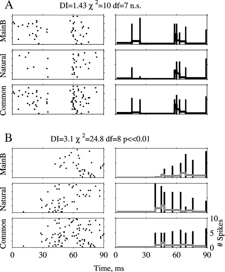
Figure 3. Calculation of the DI. A and B are two examples of a χ² test. The left column displays responses to 20 presentations of Natural and of Main Background, and their superposition, Common. The right column represents the PSTHs computed using the non-uniform bins selected as described in the text. The bars are the spike counts per bin displayed at the end point of each bin, and the gray line is the PSTH, computed by dividing the spike counts per bin by the bin duration. Scales are the same in all panels.

The expected distribution of the DI was calculated as follows. The expected distribution of a single DI value, under the null hypothesis of equal underlying rate processes for the responses to the two stimuli, was a scaled version of a χ² distribution, with the number of degrees of freedom equal to the number of bins in the underlying histograms as described above. The expected distribution of the whole set of DI values was therefore a mixture of such distributions, with the weights given by the proportion of DI values with each given number of degrees of freedom.

The distance between the observed distribution of the DIs and its expected distribution was calculated in two ways, using either the Jensen-Shannon or the Cramer-von Mises statistics. The Jensen-Shannon statistic was computed as (Lin, 1991 ):

and the Cramer-Von Mises statistics was computed as (Famoye, 2000 ):

where p_ex was the expected distribution and p_ob was the observed distribution. These distributions were computed for a bin size of 0.3–0.5 DI units, in order to have a sufficient number of counts in each bin. F_ex and Fob were the corresponding cumulative distributions computed with the same bin size. Both statistics were used since they are sensitive to somewhat different features of the differences between the distributions.

Results

In two cats, cluster activity in a large number of penetrations was used to generate spatial response maps. These responses were used to study the dependence of the responses on sound level. Furthermore, 200 well-separated neurons were recorded from 10 cats at levels corresponding to the middle and high sound levels used in the mapping experiments. Seventy-seven well-separated neurons were selected for further analysis based on their stable response during the recording session (1–2 hour). This is the same population of neurons whose responses to a related stimulus set were described in Bar-Yosef et al. (2002) . The general features of this population were described in Bar-Yosef et al. (2002) . In short, the BFs of these neurons ranged from 1 to 15.5 kHz, with 43∕77 of the neurons having BFs between 2 and 7 kHz. The clean chirps had most of their energy within the FRAs of these neurons. The neurons were typical of A1 in halothane-anesthetized cats in terms of their thresholds and tuning widths (Moshitch et al., 2006 ). The responses occurred throughout the duration of the stimulus, and on average the early and late response components (spikes occurring before and after 45 ms after stimulus onset) were not significantly different from each other (see Bar-Yosef et al., 2002 for details).

Examples of responses

Figures 4 , 5 , and 6 present responses of several neurons to natural stimuli and their modifications. In each figure, the FRAs are plotted at the top. Overlying the FRA, the power spectra of the Main (magenta) and the Noise (green) stimuli are plotted in thick lines. The responses are plotted below both as raster displays and as PSTHs, normalized in each case to the maximum response of each neuron over the displayed stimulus versions. The spectrograms of the stimuli are presented to the side of the corresponding responses in Figure 4 .

FIGURE 4

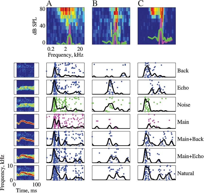
Figure 4. The responses of three neurons to the seven versions of Stimulus-3. The FRAs of the neurons are displayed in the top row (BFs: A – 2.6, B – 3.9, and C – 5.2). Each FRA is based on the responses to 45 frequencies (equally spaced on a logarithmic scale between 0.1 and 40 kHz) and 11 levels (Linearly spaced on a logarithmic scale between about 0 and 87 dB SPL). The color scale represents firing rate, where blue is 0 and red is the maximal rate of each FRA: A – 142, B – 184, and C – 285 sp∕second. The power spectra of Main (magenta) and Noise (green) at the actual level in which they were presented are plotted on top of the FRA. The left column represents the spectrograms of the versions of Stimulus-3. The responses to each version are displayed as a raster plot and as a peristimulus time histogram (PSTH). The PSTHs have been smoothed with a 10 ms hamming window. All PSTHs in a column share the same scale (A – 319, B – 80, and C – 126 sp∕second). The rasters of the responses to Main and to Noise are plotted with the color used to represent their power spectrum.

Figure 4 presents the responses of three neurons to Stimulus-3. The three neurons had a BF within the frequency range of the chirps. The neuron in Figure 4 A showed a small but significant increase in total spike counts as stimulus energy increased. For example, the total number of spikes evoked by Natural was larger than the total number of spikes evoked by Main, which was larger than the number of spikes evoked by Background. This was the expected pattern of responses of neurons whose responses were primarily determined by stimulus energy, although the differences between the responses to the various stimulus versions were not very large. Such neurons were however the exception. The neuron in Figure 4 B was probably sensitive to the echo component, since it responded to all the versions containing this component (Natural = Main + Echo + Background, Main + Echo, Noise = Echo + Background, and Echo) with a larger spike count than to the other versions, although the temporal pattern of these larger responses varied to some extent. The neuron in Figure 4 C responded to every stimulus that included Background with a robust onset response, suggesting that the onset response was due to the background component. In the same neuron, both Main and Echo, that did not include the Background component, evoked a response with substantially later onset and smaller maximal firing rate (although their sum, Main + Echo, evoked an early onset response). The responses to Natural and to Main Background contained, in addition to the onset response, a late response component possibly due to the presence of the Main component, but with a different timing than the response evoked by Main alone. Thus, it appears that the background component had an inordinately large effect on the response of this neuron, considering its low level.

Figure 5 presents the FRA and the responses to Stimuli 1, 3, and 5 of a neuron with a BF inside the frequency range of the chirps. The power spectra of the Main and Noise versions of Stimulus-5 are plotted on top of the FRA (magenta and red respectively). This neuron had an onset burst in the responses to the Natural versions of all three stimuli, but this onset burst was missing in the responses to the Main version. Tracing this response component through all versions, it seems that it was again due to the Background component.

FIGURE 5

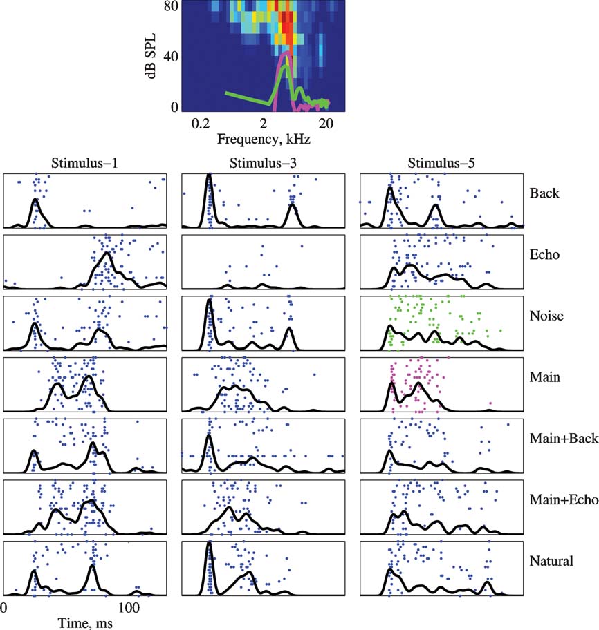
Figure 5. The responses of a neuron to the 7 versions of Stimulus-1, 3, and 5. Same conventions as in Figure 4 . The BF was 5.3 kHz and maximal firing rate in the FRA is 133 sp∕second. The PSTHs are normalized to 105 sp∕second. The power spectrum of Stimulus-5 is plotted on top of the FRA.

A similar pattern is found in Figure 6 . The power spectra plotted on the FRA are those of the Main and Noise versions of Stimulus-2. The neuron responded to the Background component of all stimuli, and to all stimulus versions that included Background (Natural, Main Background, and Noise). It responded very weakly to the Echo component of all stimuli, and generally had a weak response to the Main component (except for Stimulus-4). In contrast, it responded as vigorously to Main Echo as to Natural although there may have been some differences in the temporal patterns of these responses. This neuron therefore showed two unexpected features, in line with the responses displayed in Figures 4 and 5 : first, the strong effect of Background on its responses, even in the presence of much stronger components; and second, the response to Main Echo which was much stronger than predicted by the responses to its components Main and Echo.

FIGURE 6

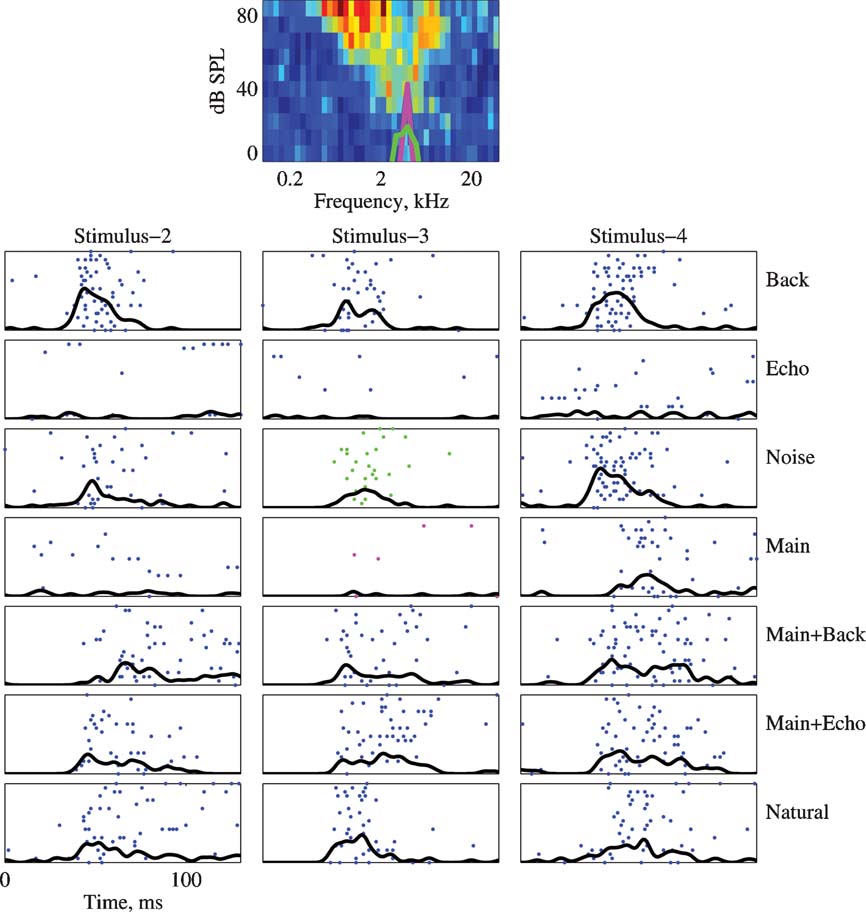
Figure 6. The responses of a neuron to all versions of stimuli 2, 3, and 4. Same conventions as in Figure 5 . The BF is 4.7 kHz. The maximal firing rate of the FRA is 260 sp∕second. The PSTHs are normalized to 130 sp∕second in all the cases. The power spectrum of Stimulus-3 is plotted on top of the FRA.

Figures 4 , 5 , and 6 illustrate two properties of the responses to this set of sounds which were observed repeatedly. First, there is no simple relationship between the FRA, the stimulus spectral energy and the neuronal response. Second, some neurons responded as though they were captured by a component of the stimuli (Main, Echo, or Background) and responded to it, even in the presence of stronger components inside their FRA.

Level dependence of the responses

In two cats, cluster responses were collected in a large number of penetrations, at two or three sound levels. Figure 7 A shows the BF maps in these two animals. In both the cases, both the anatomical markers and the regular progression of BF values demonstrate that the data are from low-frequency A1. Tuning width seemed also to be clustered in the two animals (data not shown). In both animals, wideband clusters dominated the more dorsal part of the mapped area, whereas narrowband clusters were present only in the ventral part. Thus, in both the cases, the maps probably cover the dorsal wideband area and part of the central, narrowly tuned area of A1 (Read et al., 2002 ).

FIGURE 7

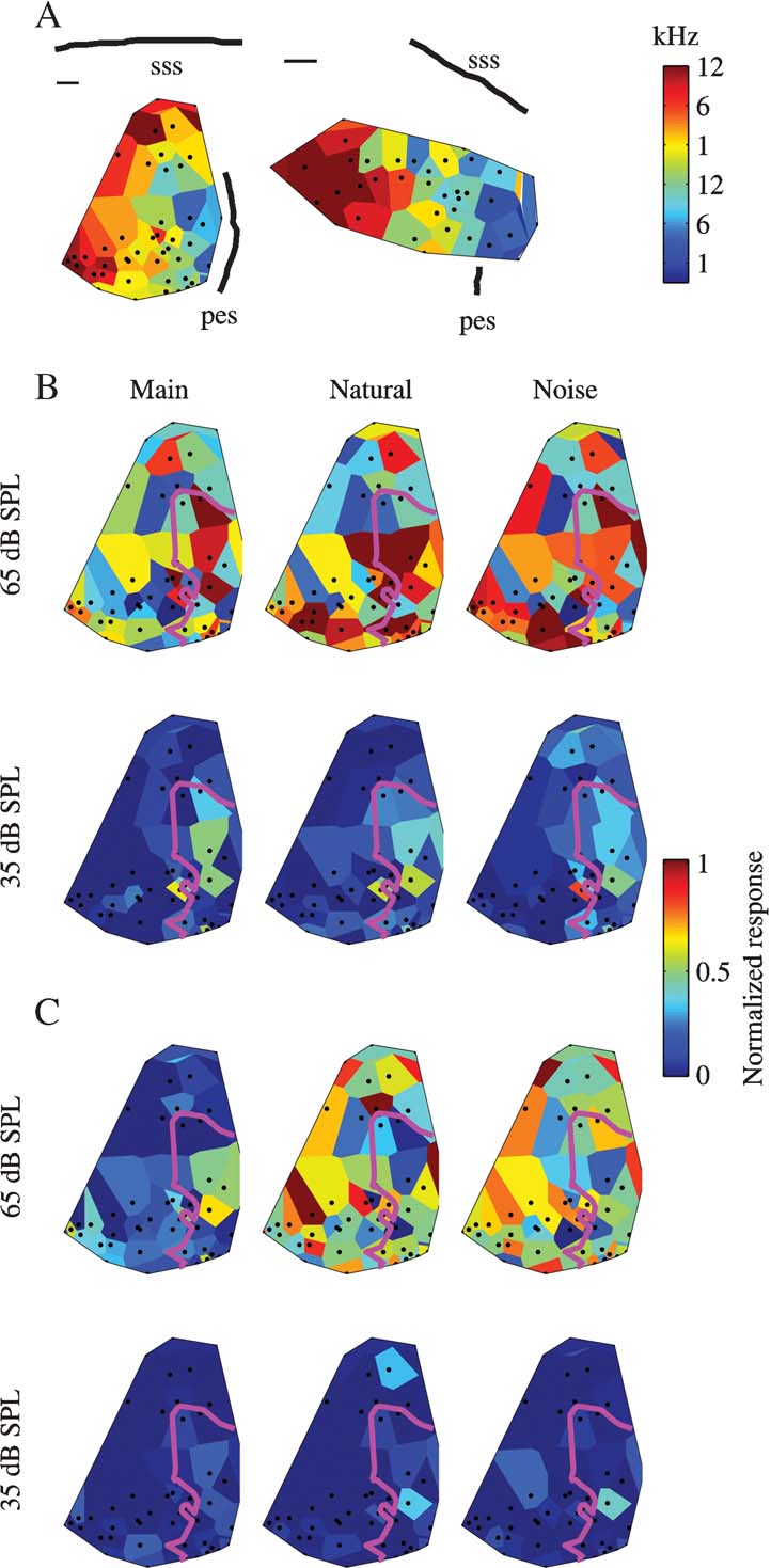
Figure 7. Topographical distributions of the responses. (A) BF maps for the two mapping experiments. Scale bars are 0.5 mm. (B) Responses to three versions of Stimulus-1 at two sound levels in one cat. The magenta line represents the 7 kHz isofrequency contour. (C) Responses to three versions of Stimulus-3 at two sound levels in the same cat as B. Same conventions as B.

The response maps to three versions (Natural, Main, and Noise) of Stimulus-1 at the lowest and highest sound level used in one experiment are shown in Figure 7 B, and the responses to the same three versions of Stimulus-3 are shown in Figure 7 C. The low sound level was such that the tonal component was at about 35 dB SPL, and the high sound level was 30 dB higher and was the same as the typical sound level used for the studies of the neural responses of well-separated single units such as those shown in Figures 4–6 .

At the low sound level, the responses were weak and mostly limited to the frequency region of the main chirps (whose border, the 7 kHz isofrequency contour, is marked by the magenta line in Figure 7 ). In Figure 7 B, the topographical distributions of the responses to Main and Natural at the low sound level are roughly similar, while that of Noise is somewhat different. In Figure 4 C, the responses are essentially non-significant. Noise generally evoked a somewhat weaker activity inside the frequency region of the main chirps, and a somewhat larger activation outside that region.

At the high sound level, the responses to all components were much larger. In the example shown in Figure 7 C, the responses to the Noise components were higher than the responses to Main, and were of similar magnitude to the responses to Natural. Furthermore, the topographical distributions of the responses to Natural and to Noise were similar to each other. In Figure 7 B, the same two effects are present, although with smaller differences between Main and Noise both in terms of the size of the responses and in terms of the similarity to the topographical distribution of the responses to Natural.

To demonstrate these results more generally, the responses were separated by sound level and stimulus. For each stimulus and sound level, the median of the normalized response to the Natural version was used as a breakpoint for separating the responses to all other versions of the same stimulus into small and large responses, where responses were considered as small if they were smaller than the median of the responses to the Natural version at the same nominal sound level, and responses were considered as large otherwise. In terms of number of evoked spikes, the criterion varied from neuron to neuron. At the low sound levels, the typical breakpoint was at a normalized rate of about 33%, corresponding to a firing rate of roughly 10 sp∕second (23 spikes∕20 stimuli; typical stimulus duration was 100 ms). At the high sound levels, the typical breakpoint was at a normalized rate of about 55%, corresponding to a firing rate of roughly 20 sp∕second (38 spikes∕20 stimuli).

The fractions of large responses for Stimulus-2 and Stimulus-3 are shown in Figures 8 A and 8 B for the two experiments respectively. The central bar in each group represents the responses to the Natural version, and its height is therefore always equal to 50% (since the breakpoint is at the median of the responses to Natural). To the left, the two bars represent the percentage of large responses to the Main + Echo and Main versions, and to the right the bars represent the percentage of large responses to the Noise and Background versions (note that in the mapping experiments, only these five stimulus versions have been used).

FIGURE 8

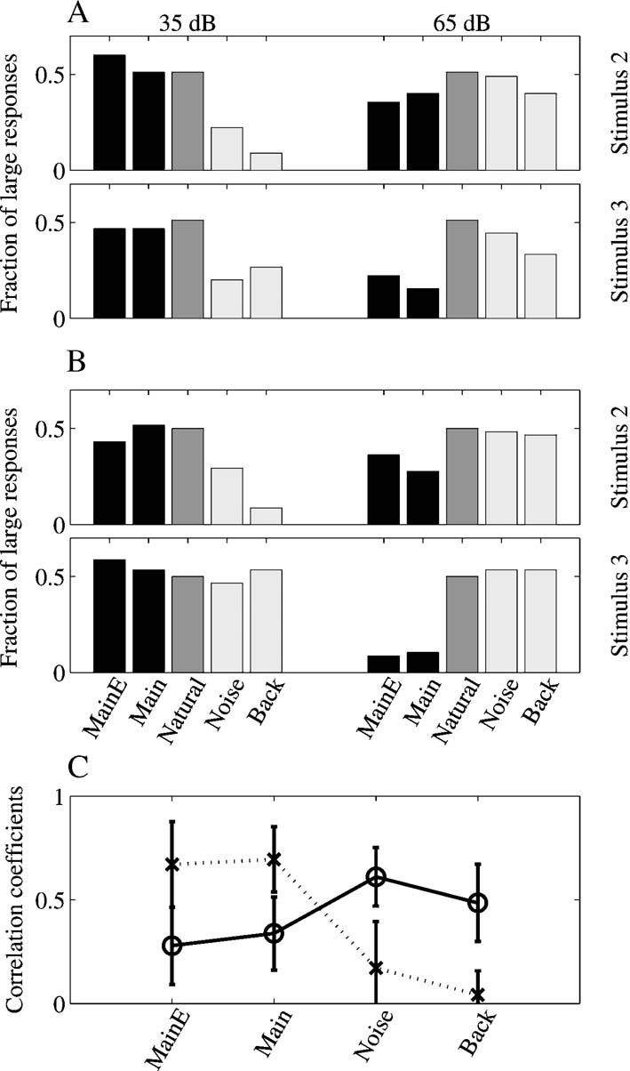
Figure 8. Quantitative analysis of the responses in the mapping experiments. (A, B) Percentages of large responses in the two mapping experiments, for stimuli 2 and 3. The middle bar (dark gray), representing the fraction of large responses to Natural, is always at 50%, the selected breakpoint between large and small responses. The two left bars in each group (black) represent the large responses to Main Echo and Main, the other two stimuli in the mapping experiments that contained the Main component. The two right bars in each group (light gray) represent the large responses to Noise and Background, the two stimuli in the mapping experiments that did not contain the Main component. (C). Average correlation coefficients between the response maps to Natural and to the other four stimulus versions used in the mapping experiments. Dotted line: maps at 35 dB, continuous line: maps at 65 dB. The error bars represent standard deviations.

At low sound levels, the fractions of large responses to Main Echo and Main are similar to the fractions of large responses to Natural, whereas the fractions of large responses to Noise and Background are generally lower. This pattern is consistent with the hypothesis that the responses are evoked by the stronger Main component, and that in general the weaker Noise and Background components did not evoke much response and did not affect much the responses to Main even when present in the sound.

On the other hand, at higher sound levels, the situation is roughly reversed: the fraction of large responses to Main + Echo and Main was generally smaller than 0.5, and the fractions of large responses to Noise and Background were close to 0.5. A one-way ANOVA on the fractions of large responses (for all stimuli and both experiments, with the stimulus version as a random factor) supports this conclusion. At both the low and the high sound levels, there is a significant difference between the fractions of large responses to the different stimuli (at 35 dB SPL: F(4,25) =7.8, p ≪ 0.05; at 65 dB SPL: F(4,25) =9.7, p ≪ 0.05). Post-hoc comparisons (at the 0.05 level) verified that at 35 dB SPL, the fractions of large responses to Noise and Background were significantly smaller than the others (Natural, Main + Echo, and Main), whereas at 65 dB SPL, the situation was the reverse, and the fractions of large responses to Main Echo and Main were significantly smaller than the other (Natural, Noise, and Background). Thus, it seems that once Noise and Background were sufficiently loud to evoke responses, they tended to dominate the Main component in spite of the difference in sound level between them.

This comparison between distributions of response magnitudes does not take into account the spatial relationships between nearby recording locations. The similarity between the responses to the various versions extended to a similarity between the spatial distributions of the responses. To demonstrate this, the correlation coefficients between the responses to the various versions in the same locations were computed. Figure 8 C shows these correlation coefficients as a function of level for the different sounds. Whereas the correlation coefficients between the responses to Natural and Main were relatively high at the low sound levels (gray line), they became smaller at the higher sound levels (black line). In contrast, the correlation coefficients between the responses to Natural and Noise were lower at the lowest sound level, but became larger at the higher sound levels.

Stimulus energy and neural response

The FRA of a neuron is a useful tool for predicting responses to some other stimuli (Heil et al., 1992a , 1992b ; Rotman et al., 2001 ; Schreiner and Sutter, 1992 ). It is often implied that the FRA is a good representation of the frequency filtering properties of the neuron, in the sense that a neuron would be activated by frequency components inside the FRA but not by frequency components outside the FRA. Because of the low spontaneous rate of most neurons, FRAs often do not represent well inhibitory subfields. Also, since FRAs are measured with pure tones, they do not reflect subthreshold convergence across frequency which may be an important factor in shaping cortical responses to broadband stimuli. As long as such non-linearities are not very important, a correlation should exist between the neuronal responses on the one hand and the overlap between stimulus spectrum and FRA (“spectral overlap”) on the other hand.

To test this prediction, the mean rate of the onset responses for each stimulus was compared to the predicted responses based on the FRA of each neuron. In this procedure, the predicted responses were derived from the spectral overlap between the initial 30 ms of each stimulus and the FRA of the neurons, and the observed responses were the spike counts in the 45 ms following stimulus onset. Only 35% (20∕57) of the adjusted correlation coefficients between the spectral overlaps and the observed responses were significant at the 0.05 level, and all of them were smaller than 0.5 (accounting for less than 25%of the variance). As mentioned above, this could be due to the fact that many neurons had long response latencies to at least some of the stimuli (e.g., the responses in Figure 6 ). Therefore, the temporal windows for the calculations of the predicted and actual responses were shifted to fit the latency of each response individually. Figure 9 A presents the adjusted correlation coefficients between spectral overlaps and observed responses using the individually determined temporal windows. Only a slightly larger number, 42% (24∕57) of the adjusted correlation coefficients were significant using this more complicated procedure. All the significant correlations were positive. There was no effect of the BF of the neuron on the correlation coefficients, as is shown by the distribution of significant and non-significant adjusted correlation coefficients as a function of BF in Figure 9 B (χ² = 10.5, df = 11, n.s.).

FIGURE 9

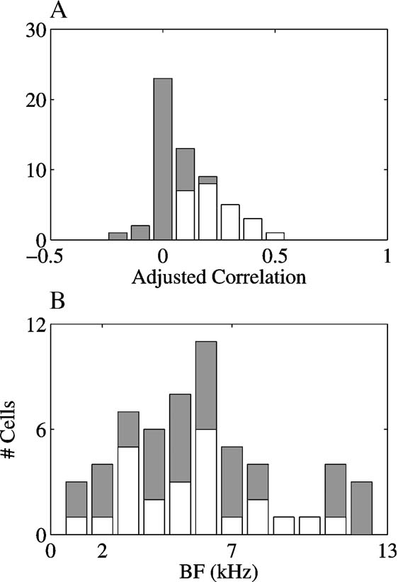
Figure 9. The adjusted correlations between the spectral overlaps of the stimuli with the FRAs and the observed responses. (A) the distribution of the adjusted correlations. (B) the distribution of the adjusted correlations as a function of BF. In both A and B, white bars represent the number of significant correlations and gray bars on top of the white bars are the number of non-significant correlations.

The distribution of the adjusted correlations between the spectral overlaps of the stimuli and the FRAs on the one hand and the observed responses on the other hand, displayed in Figure 9 A, quantifies the low predictive value of FRA for our stimuli (documented as well in Bar-Yosef et al., 2002 ). These results might arise from the sensitivity of the neurons to the background noise, shown in Figures 4–6 . The background noise could elicit a strong response even in neurons whose BFs were inside the chirp frequency range, although it had substantially less energy than the main chirp in this frequency region.

To test whether this effect was the reason for the low predictive value of the FRA, the spectral overlaps of Main and Noise with the neuronal FRAs, and the observed response to Main and Noise, were compared across neurons. In this comparison, the first 30 ms of the stimulus and the first 45 ms of the responses were used. The spectral overlaps of Main and Noise, averaged over the entire neuronal population, were not significantly different (F(1,660) =2.1, n.s.), whereas the observed responses to Noise were significantly larger than the responses to Main (F(1,660) =39.8, p ≪ 0.01). Such a result could theoretically arise from the presence of neurons whose BFs did not intersect the chirp frequency range. The same procedure was therefore performed separately for neurons with BF within and outside of the frequency range of the chirps.

In the case of neurons whose BFs were far from the chirp frequency range the expected result was found: the spectral overlap of Noise with the FRAs was significantly larger than that of Main (F(1,249) =3.6, p ≪ 0.01) and correspondingly the observed responses to Noise were also significantly larger than the responses to Main (F(1,249) =16.2, p ≪ 0.01).

However, whereas the spectral overlap of Main was, as expected, substantially larger than that of Noise for neurons whose BF was within the chirp frequency range (F(1,409) =13.2, p ≪ 0.01), the opposite was true for the observed responses: Noise elicited on average a larger response than Main (F(1,409) =20.2, p ≪ 0.01). Thus, even in this subpopulation of neurons, Noise was more efficient at eliciting a response than Main.

Comparing Natural to the other stimulus versions – Spike counts

The quantitative analysis in Figure 9 suggests that there is only a weak relationship between the spectral overlap and the strength of the responses of the neurons. The examples in Figures 4 , 5 , and 6 suggest that this finding is at least partially due to the inordinately large effect on the neuronal responses of adding a low-level component such as Background to Main, an effect which could not be captured by the FRA. To quantify this finding, Figure 10 presents the scatter plots of the normalized responses to Natural against the responses to each of the other stimulus versions. The results of the comparisons of the mean responses and the adjusted correlation coefficients are presented in Table 1 for the whole population as well as for the subpopulations separated by their BFs (within or outside of the frequency range of the chirps). The data points corresponding to the responses of the neurons presented in Figure 4 are indicated in Figure 10 , together with their standard deviations. The substantial distance between these data points and the diagonal in many cases indicates that the large scatter is real and is not solely due to estimation noise.

TABLE 1

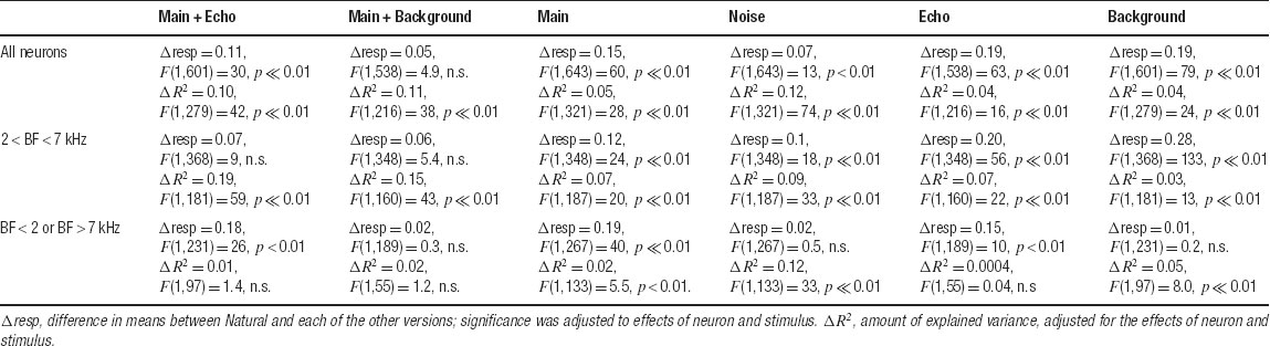
Table 1. Significance of differences of means and corelation coefficients for the scatter plots in Figure 10.

FIGURE 10

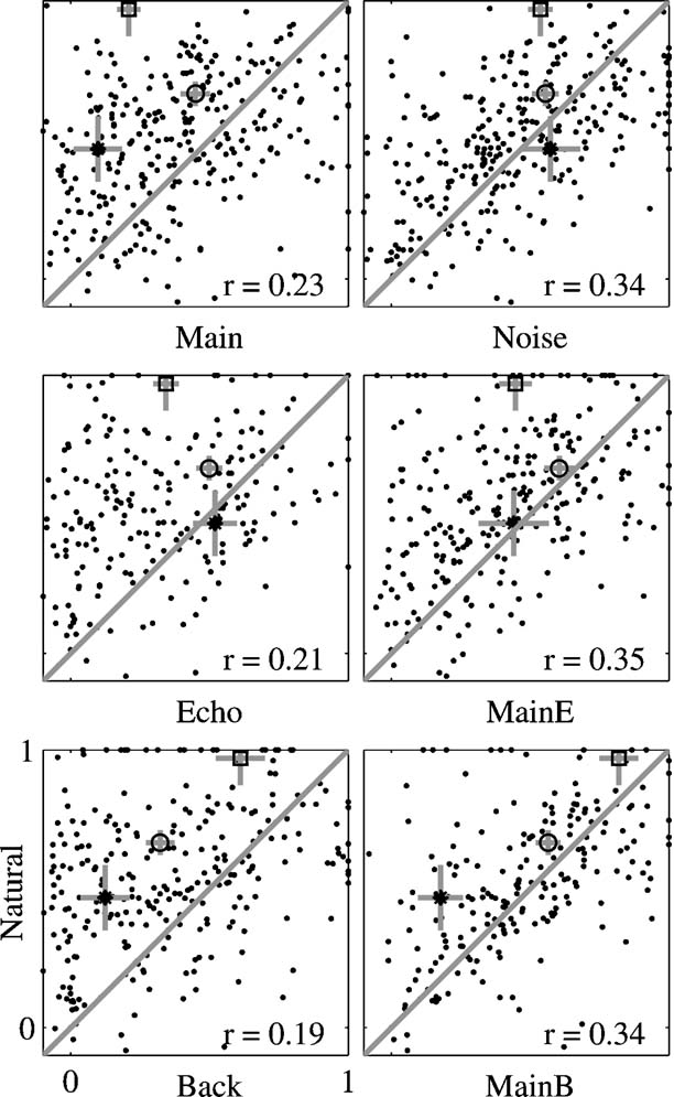
Figure 10. Scatter plots of the responses to Natural against the responses to all other stimulus versions, for the whole neuronal population. The correlation coefficient was adjusted for the effects of neurons, stimuli, and versions. The adjusted correlation is shown in each plot. The responses of the examples presented in Figure 4 are marked by the following symbols: A – circle, B – star, and C – square. The gray bars on these points are one standard error long.

In general, the responses of the entire population to Natural were stronger or equal on the average to the responses to all other stimulus versions. Main Background evoked responses that were on average the closest to those of Natural. Furthermore, the adjusted correlation coefficients between the responses to Natural and the responses to the one-component versions (Main, Echo, and Background, left panels in Figure 10 ) were smaller than those of the two-component versions (Main + Echo, Main Background, and Noise, right panels in Figure 10 ), although all were rather small. Thus, the neuronal population “distinguished” between all stimulus versions, in spite of their acoustic similarity.

The analysis restricted to the neurons whose BFs was within the frequency range of the chirps showed a similar reduction in the responses to Main Echo and Main Background relative to Natural, although the reduction was not significant for this subpopulation. However, even within this subpopulation, there was still a strong effect of the weak background components on the neural responses. For example, the amount of variance of the responses to Natural explained by the responses to Main Background was double that explained by the responses to Main, and whereas the responses to Main were significantly smaller on average than those of Natural, the responses to Main Background were much more similar to those of Natural on average.

For the neurons whose BFs were outside the chirp frequency range, the pattern of the results was simpler: every stimulus version that contained the Background component (Main Background, Noise, and Background) had on the average similar responses to Natural. The responses to Noise had the largest adjusted correlation coefficient with the responses to Natural. The responses to Main Background and Background had significant, but much smaller, correlation coefficients.

The results displayed in Table 1 suggest that whereas neurons actually responded to the part of the stimulus that intersected their FRA, the details of these responses were strongly dependent on the entire structure of the stimulus and could not be reduced to simple energy summation.

To further test this conclusion, the responses to Natural were regressed against the responses to those stimulus versions that sum up to Natural: Main Echo with Background, Main Background with Echo, Main with Noise, and Main with Echo and Background (Figure 11 and Table 2 ). In almost all the cases, the weight assigned to the two-component version (Main Echo, Main Background, or Noise) was larger than that assigned to the one-component complementary version (Main, Echo, and Background), mirroring the higher correlation coefficients between the responses evoked by the two-component stimuli and the responses to Natural. The one exception was the regression limited to those neurons whose BFs were outside the frequency range of the chirps, for which the weight of Background was larger than the weight of Main Echo (Table 2 ). In the regression of the responses of Natural on the three 1-component versions (Main, Echo, and Background), the weights of the three components were small and approximately equal, mirroring again the small and roughly equal correlation between the responses to these components and the responses to Natural.

TABLE 2

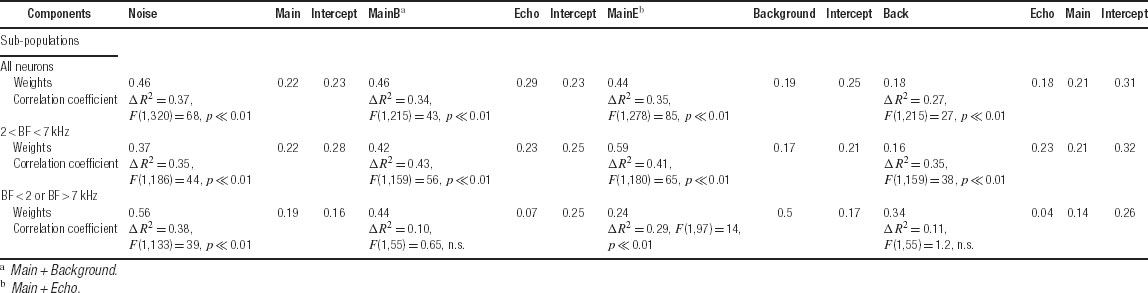
Table 2. Linear regression analysis of the spike counts evoked by Natural against the spike counts evoked by stimulus combinations that sum to Natural..

FIGURE 11

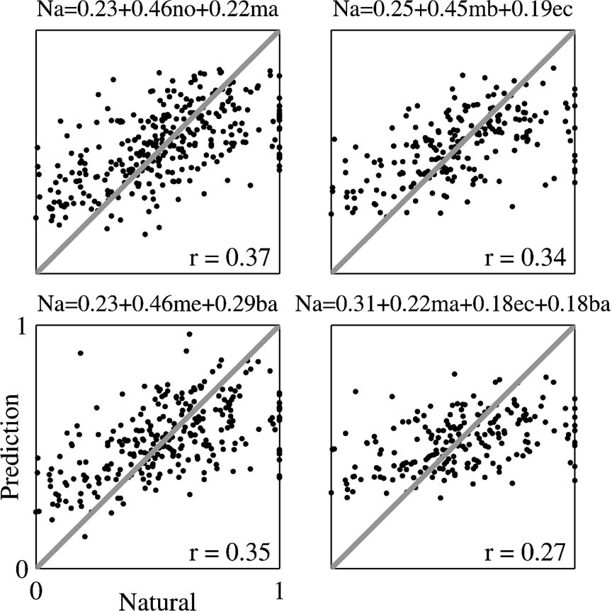
Figure 11. Scatter plots of the responses to Natural against the predictions of the linear regression equations. The linear regression coefficients were computed using the entire neuronal population. The equation of the linear regression is shown on top of each plot. The correlation coefficient between the resulting predictions and the actual responses is shown in each plot; it is adjusted for the effects of neurons, stimuli and versions. Na, me, mb, ma, no, ec, and ba represent the normalized responses to Natural, Main Echo, Main Background, Main, Noise, Echo, and Background respectively.

The fact that in the regression of the responses to Natural on the responses to Main and Noise the weight assigned to Noise is larger than the weight assigned to Main is again an indication of the significant role played by the Noise component in shaping the responses to Natural, even when the spectral overlap with Main is larger.

Comparing Natural to the other stimulus versions – Temporal response patterns

The comparison of spike counts is not sensitive to the temporal pattern of the responses. For example, in Figure 6 some responses had similar total spike counts but different temporal patterns. The temporal pattern of the responses to two stimuli was compared by a χ² test between the PSTHs of the responses to pairs of stimuli (See Materials and Methods and Figure 3 ).

Figure 12 displays the histograms of the DIs for the comparison of the responses to Natural and the responses to the other six stimulus versions. The expected distributions under the null hypothesis, that the two responses that were compared were produced by the same rate process, are superimposed in gray.

FIGURE 12

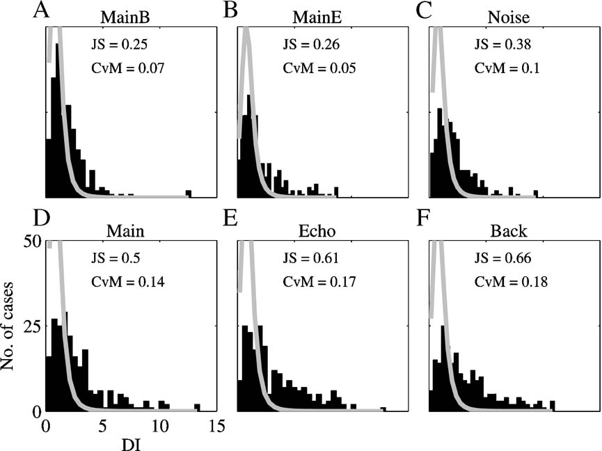
Figure 12. The distribution of the DI between Natural and all other versions. The histograms are the distribution of the DIs between the responses to six versions of all the stimuli and the responses to Natural. The gray line is the expected distribution under the null hypothesis of similarity between the responses. The distances between the observed and the expected distribution are indicated in the right corner. JS – Jensen-Shannon statistics and CVM – Cramer-von Mises statistics.

We measured the distance between the expected and measured distributions of the DIs in two different ways, both giving the same pattern of results. The distributions of the DIs for the two-component stimuli (Main + Echo, Main + Background, and Noise) were more similar to their expected distribution under the null hypothesis than the distributions of the DIs for the single component stimuli. In particular, the DI distribution for the responses to Noise was more similar to its expected distribution than the DI distribution for the responses to Main. Thus, overall, the responses to Natural were more similar to the responses to Noise than to the responses to Main.

We also wanted to directly measure the tails of the DI distributions, counting those responses whose temporal patterns deviated sharply from that of Natural. To do this, the number of DIs that exceeded the 90%point of the expected distribution was determined for each stimulus version. The results are given in Table 3 . The smallest number of large DIs (with respect to the responses to Natural) was found for Main Background and Noise, whereas the number of large DIs was larger for Main, Echo, and Background, the single component stimuli. In the subpopulation of neurons whose BFs were inside the chirp frequency range, Main and Background had a substantial number of large DIs. The large number of highly divergent responses to Main and Natural is striking because of the similarity in their acoustic structure. Conversely, Noise evoked responses that were generally similar to Natural, and within the same subpopulation of neurons the Echo sub-component of Noise was apparently responsible for this similarity. The neurons whose BFs were outside the chirps frequency range had a pattern of large DIs that was similar to the general population. Main Background and Noise had the smallest number of highly divergent responses, and both Echo and Background had a very large number of divergent responses.

TABLE 3

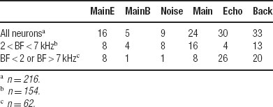
Table 3. The number of DI values larger than the 90% cutoff point for the expected distributions..

The greater similarity between the responses to Natural and Noise, relative to the responses to Natural and Main, is a common finding of both the analyses of the spike counts and the temporal patterns. This finding is unexpected because of the considerable difference between the acoustic structure of Natural and Noise, and the similarity of Natural and Main. To illustrate this similarity directly with raw data, Figure 13 presents the responses of four neurons to Natural, Main, and Noise. The neurons in Figures 13 A and 13 D had a substantially stronger response to Natural and Noise than to Main. The neuron in Figure 13 B had similar response strength to all three stimuli, but the temporal patterns of the responses were different. The neuron in Figure 13 C did not respond to either Natural or Noise, but responded robustly to Main.

FIGURE 13

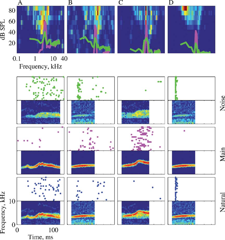
Figure 13. The responses of four neurons to Natural, Main, and Noise. The panels are arranged as in Figure 4 . The BF, FRA maximal rate, and the stimulus are: A – 2.3 kHz, 65 sp∕second, Stimulus-1; B – 5.2 kHz, 68 sp∕second, Stimulus-5; C – 5.9 kHz, 83 sp∕second, Stimulus-3; and D – 5.2 kHz, 262 sp∕second, Stimulus-5.

Sound onset and first-spike latency

Heil studied first spike latency and spike count of the onset burst in response of A1 neurons of barbiturate-anesthetized cats to pure tones at BF (Heil, 1997a , 1997b ; Heil, 1998 ; Heil and Neubauer, 2003 ). Heil and Neubauer (2003) accounted for these results by positing that first spike latency is determined by a threshold on the integrated pressure envelope. This theory successfully accounted for the first-spike latencies of neurons in auditory cortex independently of the shape of the onset ramps. Heilquotidns model accounts for first spike latency, and possibly for the number of spikes elicited during the initial burst (although this aspect of the model is limited for the highly phasic responses of cortical neurons under barbiturate anesthesia). Our data show spiking responses throughout the duration of the stimuli, which Heil's model cannot, and doesnot even try, to account for.

We used Heil's model to generate predictions for first spike latencies of our data. To do so, we have to calculate the integrated pressure envelopes. These envelopes could potentially be affected by the frequency filtering and integration processes that occur in subcortical stations. We ignored these processes here because frequency filtering limits envelope fluctuations to rates comparable with the bandwidth of the filter, and the envelopes of the stimuli used here are relatively slow. Thus, peripheral filtering is not expected to modify the results. The integrated pressure envelopes were computed by integrating the rectified waveform.

The integrated pressure envelopes are shown for three of the stimuli in Figure 14 . First spike latency should occur at a fixed integrated pressure envelope value, predicting substantially longer first spike latencies for the Echo and Background versions relative to the Main version of Stimulus-2; comparable latencies for Main and Echo but longer latencies for Background of Stimulus-3; and possible comparable latencies for all three versions of Stimulus-5. Few of these predictions hold in the data. Figure 6 displays responses to Stimulus-2, showing earlier responses to the Background version than to Main or Echo, which produced very little response. Figures 4 , 5 , and 6 have several examples of the responses to Stimulus-3. In Figures 4 C, 5 , and 6 the latency of the responses to the Background version were shortest, rather than longest, as would be predicted by Figure 14 . Only the responses to the different versions of Stimulus-5 in Figure 5 had similar latencies, possibly due to pressure integration as suggested by Heil and Neubauer. Thus, the predictions of the model are generally falsified by our data, since the responses to Main were often substantially smaller and later than those evoked by Echo, Background, or their sum, Noise.

FIGURE 14

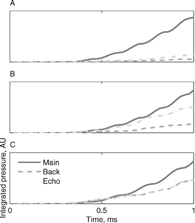
Figure 14. Integrated pressure, the main determinant of first spike latency according to Heil and Neubauer (2003) . A. Stimulus-2. B. Stimulus-3. C. Stimulus-5. First spike latency should occur at a fixed integrated pressure value, predicting substantially longer first spike latencies for the Echo and Background versions relative to the Main version of Stimulus-2; comparable latencies for Main and Echo but longer latencies for Background of Stimulus-3; and possible comparable latencies for the three versions of Stimulus-5.

In an earlier work, Heil suggested that first spike latency (and to some extent the number of evoked spikes as well) in A1 is determined by slopes or acceleration of the pressure envelope. Slopes had to be used for linear onset ramps, whereas acceleration was used for cosine onset ramps. However, these results were shown to be trivial by Fishbach et al. (2001): they resulted from the fact that the stimuli with identical slopes (or acceleration, as appropriate) were in fact initially identical, and that the spiking effectively occurred during the onset ramp.

We conclude that Heil's suggestion, which successfully accounts for thresholds of pure tones, does not account for the first spike latency of the responses to complex sounds.

Discussion

The aim of this work was to study the difference between the responses to a set of natural stimuli, consisting of bird chirps embedded in their simultaneous natural background (termed Natural here), and the responses to the same bird chirps cleaned from that background (termed Main). The initial report of these findings (Bar-Yosef et al., 2002 ) showed that contrary to expectations, the responses to Natural and to Main showed substantial differences. Here, we studied in detail these differences by using additional versions of the natural sounds. In particular, we report here in depth the responses to the background components (Noise and its subcomponents, Echo and Background) alone and in combination to the main chirp. Using this approach, we demonstrated the strong effects of the background components on the neuronal responses. In particular, we showed that when combining Main and Noise, the dominant component in shaping the neuronal responses was Noise, in spite of its lower level.

Responses to natural chirps are strongly affected by acoustic background

Two findings emphasize the importance of auditory backgrounds in shaping the responses of cortical neurons. The first is the effect of the background noise on the size of the responses, which is much larger than predicted by the spectral overlap between the power spectrum of the stimuli and the FRA of the units. The second is the greater similarity between the temporal response patterns of Natural and Noise relative to the similarity between the response patterns to Natural and Main. These effects could be shown in raw data (e.g., Figures 4–6 and 13 ) and were demonstrated quantitatively both for spike counts (Figures 10 and 11 ) and for temporal response patterns (Figure 12 ). Indeed, even in the subpopulation of neurons whose BFs were within the chirp frequency range, the similarity between the responses to Natural and to Noise was greater than the similarity between the responses to Natural and to Main.

The phenomenon described here is similar in a sense to the “strong signal capture” found by Phillips and Cynader (1985) . They used mixtures of pure tones and BBN, varying the levels of both, and showed that the responses of A1 neurons were dominated by the component that was more effective in eliciting a response when presented by itself. On average, this was also true here: the responses to Noise were stronger than the responses to Main, and the responses to Natural were more similar to the responses to Noise than to the responses to Main. However, in individual cases this was not necessarily true. For example, the neurons in Figures 5 and 13 C responded more strongly to Main than to Noise, yet their responses to Natural were more similar to their responses to Noise. Thus, it is probably a particular combination of acoustic features of the stimuli that determined the similarity in the responses, rather than the strength of the responses that these stimuli evoked (as expected from “strong signal capture”).

The claim that the background components have an inordinately large effect on the responses to the main chirp relies partially on the use of the FRA to account for the neural responses. The FRA often doesnquotidnt reflect well inhibitory sidebands, and is furthermore insensitive to subthreshold convergence of many small inputs which would result in multiple-tone facilitation of the responses to wideband stimuli.

Inhibitory areas would affect mostly the responses to wideband stimuli, reducing them relative to the expected responses based on the FRA predictions. Our findings were precisely the opposite: the background components elicited substantially larger responses than expected, and often dominated the responses even when presented in combination of substantially stronger narrowband components. Thus, inhibitory sidebands do not seem to be an important factor in shaping the responses of the neurons to this set of sounds.

The high sensitivity of the neurons to the background components suggests the presence of substantial multi-tone facilitation, indicating the importance of subthreshold convergence of weak inputs across a wide frequency range on these neurons. However, such explanation is also at best only partial: in another study, Las et al. (2005) studied the opposite situation, where the strong sound was a fluctuating wideband noise and the weak sound was a pure tone. The addition of the tone to the noise strongly affected the neuronal responses, and made them more similar to the response to the tone alone. Thus, in the conditions of the experiment of Las et al. (2005) , a low-level tone could dominated the responses of the same type of neurons, in spite of their strong responses to noise.

The stimulus version that by itself gave rise to the most similar responses to Natural was Main Background, although overall the differences between the responses to Main Background and to Noise were not large. Both Main Background and Noise are composed of a narrowband component and a wideband component: in Main Background, these are the main chirp and the background noise, and in Noise these are the echoes and the background noise. The fact that Main Background was the closest version to Natural in terms of neuronal responses, and that the responses to Noise were more similar to the responses to Natural than originally expected, suggest that the crucial step in generating the responses to Natural is the integration of the responses to the narrowband and the wideband components, an integration that is highly non-linear (e.g., Figure 11 ). Thus, we hypothesize that in addition to the fact that the FRA doesnot reflect well the integration mechanisms underlying the noise responses, it also does not reflect the presumed non-linearity in the integration of simultaneous wideband and narrowband components.

Implications

Both in the present study and in Las et al. (2005) , adding a weak sound to a strong sound resulted in responses that resembled the responses evoked by the weak sound alone. Together with Las et al. (2005) , the present study suggests that the representation of weak acoustic components may be substantially stronger in A1 than expected based on their acoustic structure.

Las et al. (2005) showed that in their case, over-representation of weak acoustic components did not occur yet in the inferior colliculus, was present in the auditory thalamus but became fully expressed in cortex. Similarly, using a subset of the data analyzed here, Chechik et al. (2006) showed a large decrease in coding redundancy in small sets of neurons in MGB and A1 relative to IC. In IC, neurons with similar BFs tended to respond similarly to these stimuli, whereas in MGB and A1 even neurons with the same BF could have substantially different response profile across these stimuli.

These results suggest that whereas in IC, stimuli are still generally represented in terms of their low-level acoustic characteristics, something else occurs in the thalamo-cortical segment of the auditory system. The increasing complexity of spectro-temporal integration in auditory cortex results in the enhancement of the representation of weak acoustic components, even in mixtures that contain substantially more intense sounds within the sensitive frequency range of the neurons.

One appealing interpretation of these data is that neurons in auditory cortex participate in auditory object segregation. Under this interpretation, the complex, non-linear integration mechanisms that operate in auditory cortex result functionally in a partial representation of sounds in terms of auditory objects, rather than in terms of spectro-temporal distributions of sound energy.

Conflict of Interest Statement

The authors declare that the research was conducted in the absence of any commercial or financial relationships that could be construed as a potential conflict of interest.

Acknowledgements

The authors thank Yaron Rotman and Liora Las for help in collecting the data. This research was supported by grants from the Israeli Science Foundation, the Volkswagenstiftung, and from the Human Frontiers Scientific Program.

References

Bar-Yosef, O., Rotman, Y., and Nelken, I. (2002). Responses of neurons in cat primary auditory cortex to bird chirps: effects of temporal and spectral context. J. Neurosci. 22, 8619–8632.

Pubmed Abstract | Pubmed Full Text

Bizley, J. K., Nodal, F. R., Nelken, I., and King, A. J. (2005). Functional organization of Ferret auditory cortex. Cereb. Cortex.

Pubmed Abstract | Pubmed Full Text

Creutzfeldt, O., Hellweg, F. C., and Schreiner, C. (1980). Thalamocortical transformation of responses to complex auditory stimuli. Exp. Brain Res. 39, 87–104.

Pubmed Abstract | Pubmed Full Text

Famoye, F. (2000). Goodness-of-fit tests for generalized logarithmic series distribution. Comput. Stat. Data Analysis 33, 59–67.

Gehr, D. D., Komiya, H., and Eggermont, J. J. (2000). Neuronal responses in cat primary auditory cortex to natural and altered species-specific calls. Hear. Res. 150, 27–42.

Pubmed Abstract | Pubmed Full Text

Heil, P. (1997a). Auditory cortical onset responses revisited. I. First-spike timing. J. Neurophysiol. 77, 2616–2641.

Pubmed Abstract | Pubmed Full Text

Heil, P. (1997b). Auditory cortical onset responses revisited. II. Response strength. J. Neurophysiol. 77, 2642–2660.

Pubmed Abstract | Pubmed Full Text

Heil, P. (1998). Further observations on the threshold model of latency for auditory neurons [comment]. Behav. Brain Res. 95, 233–236.

Pubmed Abstract | Pubmed Full Text

Heil, P., and Neubauer, H. (2003). A unifying basis of auditory thresholds based on temporal summation. Proc. Natl. Acad. Sci. USA 100, 6151–6156.

Pubmed Abstract | Pubmed Full Text

Heil, P., Rajan, R., and Irvine, D. R. (1992a). Sensitivity of neurons in cat primary auditory cortex to tones and frequency-modulated stimuli. I: Effects of variation of stimulus parameters. Hear. Res. 63, 108–134.

Pubmed Abstract | Pubmed Full Text

Heil, P., Rajan, R., and Irvine, D. R. (1992b). Sensitivity of neurons in cat primary auditory cortex to tones and frequency-modulated stimuli. II: Organization of response properties along the ‘isofrequency’ dimension. Hear. Res. 63, 135–156.

Pubmed Abstract | Pubmed Full Text

Joris, P. X., Schreiner, C. E., and Rees, A. (2004). Neural processing of amplitude-modulated sounds. Physiol. Rev. 84, 541–577.

Pubmed Abstract | Pubmed Full Text

Kadia, S. C., and Wang, X. (2003). Spectral integration in A1 of awake primates: neurons with single- and multipeaked tuning characteristics. J. Neurophysiol. 89, 1603–1622.

Pubmed Abstract | Pubmed Full Text

Las, L., Stern, E. A., and Nelken, I. (2005). Representation of tone in fluctuating maskers in the ascending auditory system. J. Neurosci. 25, 1503–1513.

Pubmed Abstract | Pubmed Full Text

Liang, L., Lu, T., and Wang, X. (2002). Neural representations of sinusoidal amplitude and frequency modulations in the primary auditory cortex of awake primates. J. Neurophysiol. 87, 2237–2261.

Pubmed Abstract | Pubmed Full Text

Lin, J. (1991). Divergence measures based on the Shannon entropy. IEEE Trans. Inf. Theory 37, 145–151.

Machens, C. K., Wehr, M. S., and Zador, A. M. (2004). Linearity of cortical receptive fields measured with natural sounds. J. Neurosci. 24, 1089–1100.

Pubmed Abstract | Pubmed Full Text

Moshitch, D., Las, L., Ulanovsky, N., Bar-Yosef, O., and Nelken, I. (2006). Responses of neurons in primary auditory cortex (A1) to pure tones in the halothane-anesthetized cat. J. Neurophysiol. 95, 3756–3769.

Pubmed Abstract | Pubmed Full Text

Nelken, I., and Versnel, H. (2000). Responses to linear and logarithmic frequency-modulated sweeps in ferret primary auditory cortex. Eur. J. Neurosci. 12, 549–562.

Pubmed Abstract | Pubmed Full Text

Pelleg-Toiba, R., and Wollberg, Z. (1991). Discrimination of communication calls in the squirrel monkey: “call detectors” or “cell ensembles”?. J. Basic Clin. Physiol. Pharmacol. 2, 257–272.

Pubmed Abstract | Pubmed Full Text

Phillips, D. P., and Cynader, M. S. (1985). Some neural mechanisms in the cat's auditory cortex underlying sensitivity to combined tone and wide-spectrum noise stimuli. Hear. Res. 18, 87–102.

Pubmed Abstract | Pubmed Full Text

Read, H. L., Winer, J. A., and Schreiner, C. E. (2002). Functional architecture of auditory cortex. Curr. Opin. Neurobiol. 12, 433–440.

Pubmed Abstract | Pubmed Full Text

Reale, R. A., and Imig, T. J. (1980). Tonotopic organization in auditory cortex of the cat. J. Comp. Neurol. 192, 265–291.

Pubmed Abstract | Pubmed Full Text

Ricketts, C., Mendelson, J. R., Anand, B., and English, R. (1998). Responses to time-varying stimuli in rat auditory cortex. Hear. Res. 123, 27–30.

Pubmed Abstract | Pubmed Full Text

Rotman, Y., Bar-Yosef, O., and Nelken, I. (2001). Relating cluster and population responses to natural sounds and tonal stimuli in cat primary auditory cortex. Hear. Res. 152, 110–127.

Pubmed Abstract | Pubmed Full Text

Sahani, M., and Linden, J. F. (2003). How linear are auditory cortical responses?. In Advances in Neural Information Processing System 15, S. Becker, S. Thrun, and K. Obermayer, eds. (Cambridge, MA, USA, MIT Press).

Schreiner, C. E., and Sutter, M. L. (1992). Topography of excitatory bandwidth in cat primary auditory cortex: single-neuron versus multiple-neuron recordings. J. Neurophysiol. 68, 1487–1502.

Pubmed Abstract | Pubmed Full Text

Sokal, R. R., and Rohlf, F. J. (1981). Biometry,. 2 edn. (New York, W. H. Freeman).

Sovijarvi, A. R. (1975). Detection of natural complex sounds by cells in the primary auditory cortex of the cat. Acta Physiol. Scand. 93, 318–335.

Pubmed Abstract | Pubmed Full Text

Sutter, M. L., and Loftus, W. C. (2003). Excitatory and inhibitory intensity tuning in auditory cortex: evidence for multiple inhibitory mechanisms. J. Neurophysiol.

Pubmed Abstract | Pubmed Full Text

Tan, A. Y., Zhang, L. I., Merzenich, M. M., and Schreiner, C. E. (2004). Tone-evoked excitatory and inhibitory synaptic conductances of primary auditory cortex neurons. J. Neurophysiol. 92, 630–643.

Pubmed Abstract | Pubmed Full Text

Tian, B., and Rauschecker, J. P. (1998). Processing of frequency-modulated sounds in the cat's posterior auditory field. J. Neurophysiol. 79, 2629–2642.

Pubmed Abstract | Pubmed Full Text

Tomita, M., Norena, A. J., and Eggermont, J. J. (2004). Effects of an acute acoustic trauma on the representation of a voice onset time continuum in cat primary auditory cortex. Hear. Res. 193, 39–50.

Pubmed Abstract | Pubmed Full Text

Wang, X., Merzenich, M. M., Beitel, R., and Schreiner, C. E. (1995). Representation of a species-specific vocalization in the primary auditory cortex of the common marmoset: temporal and spectral characteristics. J. Neurophysiol. 74, 2685–2706.

Pubmed Abstract | Pubmed Full Text

Wehr, M., and Zador, A. M. (2003). Balanced inhibition underlies tuning and sharpens spike timing in auditory cortex. Nature 426, 442–446.

Pubmed Abstract | Pubmed Full Text