1
Physics Department, University of Buenos Aires, Buenos Aires, Argentina
2
Inserm-CEA Cognitive Neuroimaging Unit, CEA/SAC/DSV/DRM/NeuroSpin, Gif sur Yvette, France
3
Collège de France, Paris, France
Behavioral observations suggest that multiple sensory elements can be maintained for a short time, forming a perceptual buffer which fades after a few hundred milliseconds. Only a subset of this perceptual buffer can be accessed under top-down control and broadcasted to working memory and consciousness. In turn, single-cell studies in awake-behaving monkeys have identified two distinct waves of response to a sensory stimulus: a first transient response largely determined by stimulus properties and a second wave dependent on behavioral relevance, context and learning. Here we propose a simple biophysical scheme which bridges these observations and establishes concrete predictions for neurophsyiological experiments in which the temporal interval between stimulus presentation and top-down allocation is controlled experimentally. Inspired in single-cell observations, the model involves a first transient response and a second stage of amplification and retrieval, which are implemented biophysically by distinct operational modes of the same circuit, regulated by external currents. We explicitly investigated the neuronal dynamics, the memory trace of a presented stimulus and the probability of correct retrieval, when these two stages were bracketed by a temporal gap. The model predicts correctly the dependence of performance with response times in interference experiments suggesting that sensory buffering does not require a specific dedicated mechanism and establishing a direct link between biophysical manipulations and behavioral observations leading to concrete predictions.
Multiple stimuli are continuously being processed in parallel by the sensory systems, eliciting a brief transient sensory response which in most cases fades after few hundred milliseconds, without reaching working memory, executive control and consciousness. Theoretical and computational models have proposed two-stage or workspace models of information flow in perceptual tasks. The first stage involves an effortless parallel processing of multiple sensory elements and is available to the system only for a short-time. At a second stage, only a subset of the iconic buffer is amplified under top-down control, sustained and broadcasted to become accessible for conscious processing (Baars, 1989
; Chun and Potter, 1995
; Dehaene et al., 1998
).
Support for this idea comes from single-cell physiology in awake-behaving monkeys which have shown that a visual stimulus evokes a rapid transient response (the feed-forward sweep) followed by a second wave of activity, which is thought to involve recurrent processing (Lamme and Roelfsema, 2000
; Lamme et al., 2000
; Lee et al., 2002
; Li et al., 2006
; Roelfsema et al., 2000
). In absence of prior stimulus expectation or specific task-setting context, the first transient response is largely determined by stimulus properties and is unaffected by figure-ground signals, the presence of a concurrent mask or the behavioral relevance of the stimulus. On the contrary, the second wave is modulated by contextual aspects affecting the visibility of the stimulus such as figure-ground signals and is suppressed by anesthetics (Lamme et al., 1998
). For example, during a contour detection task the neural signal for contour saliency in primary visual cortex is delayed 60–100 ms relative to the outset of the neuronal response, itself unaffected by the saliency of the contour or attentional state (Li et al., 2006
). Similarly, during a memory-guided visual search task, cells in infero-temporal cortex elicit an early response and only after about 150–200 ms this response bifurcates showing an enhanced response for targets compared to distractors (Chelazzi et al., 1993
, 1998
).
In all these experiments, the latency of the second wave is determined by the intrinsic timing of the allocation of attention. The biophysical mechanisms involving this second wave are debated, and it has been argued that they involve, top-down control by feedback connections, but also, local-competition and recurrent connections within the same cortical modules (Gilbert and Sigman, 2007
).
The consequences of bracketing the stimulus presentation and the allocation of attention in an experimentally controlled temporal interval have been extensively explored in behavioral and neurophysiological experiments in human subject. Sperling and colleagues discovered that while only a few (3–5) elements from a stimulus array can be remembered, many more items can be reported when subjects are required to identify a cued subset of items at a short (less than a second) interval after the removal of the visual display (Loftus et al., 1992
; Sperling, 1960
), indicating the existence of a transient high-capacity initial memory – referred in the vision literature as iconic memory (Averbach and Coriell, 1961
; Chow, 1986
; Coltheart, 1980
; Loftus et al., 1992
; Lu et al., 2005
; Sperling, 1960
; Turvey and Kravetz, 1970
).
A second experimental strategy to separate experimentally the timing of stimulus presentation and top-down control involves dual-task interference experiments (Duncan et al., 1994
; Pashler and Johnston, 1998
; Raymond et al., 1992
). When two tasks are presented in rapid succession, and the second stimulus is unmasked, a systematic delay is observed in the execution of the second stage of the second task, a phenomenon referred as psychological refractory period (PRP) (Pashler and Johnston, 1989
; Smith, 1967
). If the second stimulus is masked, its visibility diminishes severely, even with moderate masking, a phenomenon referred as the attentional blink (AB, Raymond et al., 1992
). These two forms of interference have been combined in a common experiment (Jolicoeur, 1999
; Wong, 2002
), and it has been shown that visibility of the second stimulus decreases exponentially as the response time to the first task increases (Jolicoeur, 1999
). The temporal constant of this decay is of a few hundred milliseconds, suggesting that it may be related to the decay of iconic memory, however, the nature and biophysical specificity of this sensory memory is not understood and requires theoretical and experimental investigation.
Here we establish a biophysical model intended to bridge the partial retrieval of sensory information – as determined in partial report and AB experiments – to the two-stage organization of responses in visual areas of awake-behaving monkeys. We show that a simple model, involving a first initial transient response followed by a forced competition set out by top-down currents can account for these observations implying that there is no need to postulate a specific region or circuit for sensory buffering. The model establishes concrete predictions of the duration of this memory and of the probability of correct retrieval as experimental (the time between stimulus and top-down control, masking, stimulus strength…) and biophysical (the strength of recurrent connections and top-down currents) parameters are varied.
The cortical model used in this work has been developed by XJ Wang and collaborators (Brunel and Wang, 2001
; Wang, 2002
; Wong and Wang, 2006
). Unless mentioned, all parameters are set as in these previous studies. The external currents are varied to simulate the different experiments of interest in this study.
Spiking Network
The spiking neural network (Wang, 2002
) is composed of 2,000 (N) leaky integrate and fire neurons, Ne (total 1,600, 80%) pyramidal and Ni (total 400, 20%) inhibitory neurons. From the Ne excitatory neurons, f × Ne neurons are selective to target 1 and a non overlapping group composed of f × Ne neurons are selective to target 2. The rest of the excitatory cells [Ne × (1 − 2 × f)] are not selective to any of the two targets. Thus the network is divided in four homogeneous populations: two excitatory selective, one excitatory non-selective, and one inhibitory.
In the simulations, N = 2,000, Ne = 1,600, Ni = 400, f = 0.15.
Both pyramidal cells and interneurons are described by leaky integrate-and-fire neurons. The sub-threshold membrane potential evolves according to:
where Isyn(t) represents the total synaptic current flowing into the cell, Cm is the membrane capacitance (0.5 nF for pyramidal cells and 0.2 nF for interneurons), VL = −70 mV is the resting potential, and gL is the membrane leak conductance (25 nS for pyramidal cells and 20 nS for interneurons). When the membrane potential reaches the threshold Vtresh = −50 mV a spike is emitted, and V(t) is reset to Vres = −55 mV. Post-spike refractory period τref is 2 ms.
The network is endowed with all-to-all connectivity. All external currents including background noise, top-down and bottom-up currents are mediated exclusively by fast AMPA receptors. Recurrent excitatory currents within the module are mediated by AMPA and NMDA receptors, while inhibition is mediated by GABA receptors. The total synaptic input to each cell is given by:

in which
VE = 0 mV and VI = −70 mV are reversal potentials for excitatory and inhibitory neurons. The concentration of Mg2+ controlling the voltage dependence of NMDA currents is set to 1 mM. The sum over j represents a sum over the synapses formed by presynaptic neurons j. The dimensionless weights wj determine the structure of excitatory recurrent connections (see below).
Gating variables (fraction of open channels) are described as follows. For AMPA channels:
where τAMPA = 2 ms.  is the time of the spike k emitted by presynaptic neuron j.
is the time of the spike k emitted by presynaptic neuron j.Each neuron receives large amounts of external noise, simulated as spikes arriving to each cell independently at an average frequency of 2.4 kHz, which simulates a neuron receiving input from 800 neurons firing at a spontaneous rate of 3 Hz, independent from cell to cell. As a result of this noisy input (assumed Poisson), neurons inside the module fire at a spontaneous rate of ∼3 Hz.
As described in the “Results” section, we submit the model to a series of two stages, defined by the particular configuration of external currents (top-down, bottom-up) These two stages are separated (bracketed) in time by an experimentally controlled variable which we refer to as the buffer. In the first stage, which corresponds to the bottom-up stimulation generated by stimulus presentation, external inputs are increased for both populations of selective neurons, in 240 Hz for the population with higher selectivity and in 120 Hz for the population with lower selectivity. This stimulation lasts 100 ms and is followed by a mask, which is modeled as an increase in the external inputs to the non-selective cells from the spontaneous rate of 2.4 to 2.88 kHz, also during 100 ms. In the second stage top-down control is directed to the network, modeled as a constant increase to the external input to all excitatory cells (both selective and non-selective) from 2,400 to 2,544 Hz.
NMDA channels are described by
where the decay time of NMDA currents is τNMDA,decay = 100 ms, α = 0.5 ms−1, and τNMDA,rise = 2 ms. The GABA synaptic variable follows:
where the decay time constant of GABA currents is τGABA = 5 ms. All synapses have a latency of 0.5 ms.
The synaptic conductances adopted are (in nS): for pyramidal cells, gext,AMPA = 2.1, grec,AMPA = 0.05, gNMDA = 0.165, and gGABA = 1.3; for interneurons, gext,AMPA = 1.62, grec,AMPA = 0.04, gNMDA = 0.13, and gGABA = 1.0. These values are the same as those used by Wang (2002)
.
The network is endowed with all-to-all connectivity. Connections are structured according to a “Hebbian” learning rule: coupling strength between pairs of neurons is considered to be high for neurons inside a selective population, and low when connecting neurons from competing populations. Specifically, for synapses connecting neurons within the same selective population, a potentiated weight wj = w+ was adopted, where w+ is a number larger than one, here set to w+ = 1.66. For connections between distinct selective populations, and from non-selective to selective populations, wj = w−, where w− is a number smaller than one, is a measure of the strength of the synaptic depression. In order to maintain the spontaneous activity of the network as w+ is varied (Amit and Brunel, 1997
), w− = 1 − f(w+ − 1)/(1 − f). For all other connections w = 1.
Reduction to the Two-Node Model
The simplified model used in this work is derived by (Wong and Wang, 2006
), where a “mean-field” approach was followed to reduce the 2,000 spiking-neurons model just described to one with only two coupled differential equations capturing central aspects of the original model. Details on this derivation can be found in their original publication (Wong and Wang, 2006
).
In the two-node network, each node represents the activity of one of the two selective populations. This activity is described by the output synaptic gating variables (“proportion of open channels”), whose dynamics follows:
where i = 1, 2 identifies the selective population. τs = 100 ms, and γ = 0.641. Hi is the simplified input–output function for neuron i (Abbott and Chance, 2005
):


During stimulus presentation, bottom-up currents are increased during 50 ms according to:

where i = 1,2 identifies the population being stimulated. Bottom-up currents are step-functions and are set 100 ms after the beginning of the trial.
Also just as in the spiking model, top-down control is modeled as an increase in external currents, equally for both populations:

Top-down currents are also step-functions, and the temporal gap (buffer) between stimulus and top-down control is calculated as follows in the speeded AB simulations (Figure 4
):

The perceptual latency of the first task (P) is fixed at 50 ms. RT1 is the response time to the first task. Each of the four curves in Figure 4
A was constructed by adopting four different values for RT1, according to the averaged response times observed experimentally after binning trials in quartiles (Jolicoeur, 1999
): RT1 = [492, 592, 673, 827] ms. The stimulus onset asynchrony (SOA) is the time between the onsets of the first and second stimulus in the AB experiment. In Figure 4
, SOA = [100, 200, 300, 400, 500, 600, 700, 800] ms.
Noise is added as an additional current, described by:
where ηi is Gaussian white noise with zero mean and unit variance.
Parameters have been slightly adjusted from those in previous studies (Wong and Wang, 2006
) to replicate Jolicoeur’s (1999)
experiment.
The remaining parameter set is: a = 270(VnC)–1, b = 108 Hz, d = 0.154 s, τnoise = 2 ms, JN,11= JN,22 = 0.22 nA, JN,12 = JN,21 = 0.08 nA, JA,ext = 5.2 × 10⁻⁴ nA Hz−1, I0 = 0.3255 nA, μstim,1 = 96 Hz. μstim,2 = 64 Hz,μtd = 70 Hz, σnoise = 0.026 nA.
Numerical solutions were calculated with first-order Euler’s method, with a time step of 0.5 ms. Results were verified for time steps of 0.05 ms, with similar results.
Partial Report
In the partial report experiment the set of competing responses is composed of 26 letters. We constructed a simple model where each of these letters is represented by a variable with a normalized output in the range (0, 1). For simplicity, we neglect any interaction between letters in different positions of the stimulus array and thus the eight different locations are modeled independently.
The activity of neural populations describing each of the N = 26 possible letters in a given location is described by xj:
where Ij is the external input to population j, u is a global inhibitory input that depends on the total excitation, I0 = 0.22 is a constant input bias, and τ = 100 ms. Coefficient c(i) specify the weight of excitatory interactions between nodes of the network. We assume that c(n + N) = c(n) and that c(n) = c(−n). Each excitatory population is entailed with self-excitation and mild excitatory connections to other populations in the network with weights: c(0) = 5, c(1) = 0.4, c(2) = 0.2, and c(i) = 0 for i > 2.
F and u are sigmoid activation functions:
The noise term evolves according to:
where τnoise = 2 ms, σnoise = 0.2, and η is a Gaussian white noise with zero mean and unit variance.
As in the AB simulations, external currents are step functions. Only the stimuli presented in the visual display receive non-zero external currents during stimulus presentation (100 ms). After cue onset, which identifies the location of the target, all excitatory connections in the target location receive excitatory input. A constant delay of 230 ms is assumed between cue presentation and top-down control. We used the following amplitudes for external inputs:
The solid curve in Figure 5
D was obtained by fitting the model simulations to an exponential distribution (R2 > 0.995). Data for the fit was obtained by averaging 3,000 simulations at each of 43 inter-stimulus-cue intervals (from 0 to 1,050 ms at intervals of 25 ms).
At long stimulus-cue delays performance reaches a plateau of around p∞ = 0.45 (Graziano and Sigman, 2008
) (Figure 5
D). In our simulations, in which we strictly model the gain of iconic memory, the visual-display decays exponentially, yielding a performance p(t) which results in chance performance for long stimulus-cue intervals and thus cannot explain the asymptotic performance to a non-chance level.
To account for this fact, we chose the simplest model of attention distribution in which a subject spontaneously allocates top-down to a random portion of the visual field and then shifts if the cue did not coincide with the chosen location. The probability that the cued location falls inside the spontaneous window of attention (pw) can be estimated from performance at long stimulus-cue delays:
where N = 26 is the number of alternative responses and p∞ = 0.45 is the experimental plateau performance at long inter-stimulus-cue intervals. This measure can be used to correct p(t) – i.e. to relate the iconic memory gain to true performance in the partial report paradigm experiment, according to:
Bracketing Stimulus Presentation and Top-Down Control: Motivation and Objectives
We simulated the dynamics of sensory information in a neuronal circuit which is submitted to a sequence of two stages, each defined by a distinct operational mode of the same circuit. The first stage (Load) corresponds to the stimulus presentation. In the second stage (Retrieval) the system receives top-down currents which amplify the response forcing a decision.
We studied a network similar to the one proposed by Wang (2002)
, composed of 2,000 leaky integrate and fire neurons (80%) pyramidal and (20%) inhibitory neurons. The excitatory neurons are divided in those selective to target 1, to target 2, and non-selective (selective to other targets not explored in the simulations). The network is endowed with all-to-all connectivity. All external currents including background noise, top-down and bottom-up currents are mediated exclusively by fast AMPA receptors. Recurrent excitatory currents within the module are mediated by AMPA and NMDA receptors, while inhibition is mediated by GABA receptors. Coupling strength between pairs of neurons is higher between neurons inside a selective population. We decided to implement and study a detailed biophysical model to explore the relation between biophysical parameters and behavioral observations. Unless otherwise noted, the results reported in this paper are robust to parameter manipulations and did not require explicit parameter fine-tuning. We thus decided to use the set of parameters which have been previously used in the literature (Wang, 2002
).
We performed a simulation of the network in which load and retrieval are separated by a brief temporal interval. This represents a very simple model of visual experiments in which relevant and irrelevant information compete in the visual scene. As described in the introduction, contour grouping and visual search are examples of such tasks (Figures 1
A,B). We did not intend here to model the specific architecture of these tasks but rather to provide a general framework for the interaction between bottom-up information and top-down control. The initial load consists on the stimulation of a small number of selective neurons, which are followed by a mask modeled as a brief excitation of non-selective cells, which succinctly represent the side-inhibition of the clutter field of distractors (Figure 1
C,E). After a small hiatus (set to 300 ms from stimulus offset in Figure 1
B) top-down control is directed to the network. Top-down is modeled as a global current injected to all excitatory neurons. The dynamic mechanisms involving the spontaneous engagement of such system, involving saliency maps, task relevance etc… are not modeled here and will be explored in further studies. The dynamics of the populations selective to the stimulus reproduces accurately the experimental data. This result was expected and does not present much novelty since it had been already shown that this network results in different operational modes as the input current to the circuit is varied. In the absence of currents, the system rests quiescent. In the presence of external currents, it can undergo a bifurcation leading to persistent activity (Wong and Wang, 2006
).
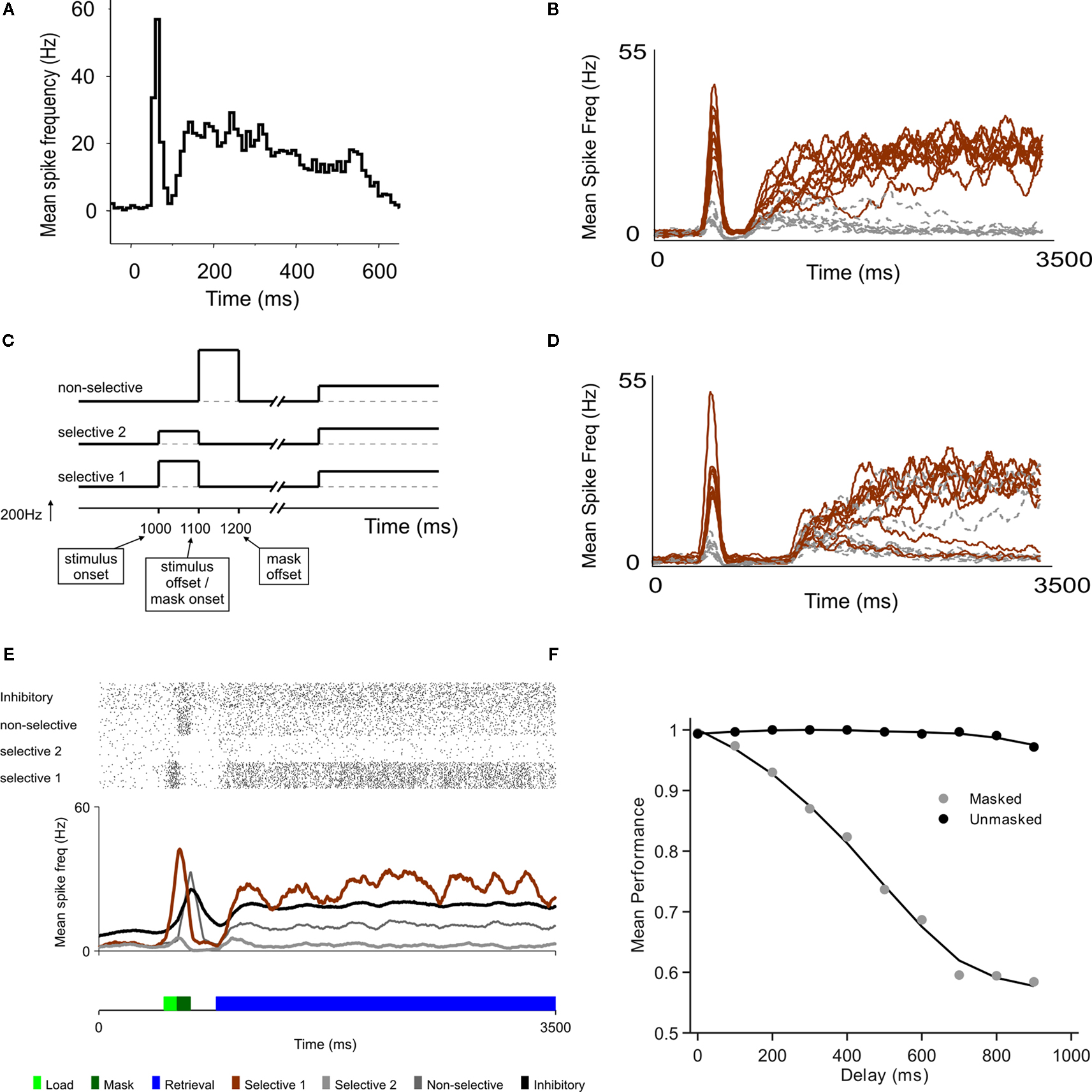
Figure 1. A model of sensory decay and top-down memory retrieval. (A) Neural recording in area V1 from a monkey performing a contour grouping task (Li et al., 2006
), showing a first initial transient followed by a second wave of delayed activations. (B) Two-stage responses in a recurrent model of cortical processing. Top-down control, which sets the circuit in a winner-take-all mode, is directed to the network 300 ms after stimulus offset. The average firing rate of selective (brown) and non-selective (grey) populations are plotted (firing rates are averaged in causal windows of 100 ms and sliding steps of 5 ms). (C) Schematic time course of input signals. The model is submitted to a series of two stages, defined by the particular configuration of external currents (top-down, bottom-up). In the first stage, which corresponds to the bottom-up stimulation generated by stimulus presentation, external inputs are increased for both populations of selective neurons, in 240 Hz for the population with higher selectivity and in 120 Hz for the population with lower selectivity. This stimulation lasts 100 ms and is followed by a mask, which is modeled as a stimulation of non-selective cells also during 100 ms. In the second stage, after a delay which is under experimental control, top-down control is directed to the network, modeled as a constant input to all excitatory cells. (D) Predicted neural activations of an electrophysiological experiment that has not been done, bracketing stimulus presentation and top-down control. The duration of the buffer is 700 ms. (E) The excitatory neurons are divided in those selective to target 1, to target 2, and non-selective. Visual masking (dark green box) is represented as a stimulation of excitatory non-selective cells that through shared inhibitory connections increase the decay rate of the stimulus trace. A raster plot of representative (randomly selected) neurons of all populations is shown, as well as the average activity of each group. (F) Proportion of correct retrievals as a function of the duration of the perceptual buffer, for trials with and without backwards mask.
The main aim and novelty of this study is to understand the dynamics of information when – as done in the partial report paradigm experiments – stimulus presentation (and the evoked transient response) and top-down control are bracketed by a controlled temporal interval. When top-down currents are injected, the network becomes bistable, with one selective population active and the other inhibited.
In all trials one population receives a stronger current during stimulus presentation (see Figure 1
C). A trial is considered correct when the active population after retrieval corresponds to the more stimulated population. For short delay between stimulus offset and top-down control (300 ms, Figure 1
B), the more stimulated population (black trace) was amplified with high probability. For a larger delay (700 ms, Figure 1
D), the transient stimulus fades out and in a more substantial amount of trials, the less-stimulated population (grey trace) was amplified during retrieval.
The probability of correct response as a function of the delay decreased, reaching a plateau about 1 s following stimulus presentation (Figure 1
F). Interestingly, in consistency with experimental observations (Giesbrecht and Di Lollo, 1998
), when the stimulus in unmasked it can be retrieved independently of the buffer duration (Figure 1
F).
The objective of these simulations – of an electrophysiological experiment which has not been performed – is to understand in more detail the probability of correct retrieval as a function of stimulus properties (strength, specificity, duration) and of the temporal interval – henceforth referred simply as the buffer (Figure 1
C). To provide a more quantitative understanding, it is useful to collapse this broad network into the smallest number of relevant dimensions through mean-field and dimensionality reduction (Wong and Wang, 2006
).
Bracketing Stimulus Presentation and Top-Down Control: Description of the Model
Previous studies have shown that a two-node network can embody in simplified but accurate form the dynamics of the large-scale cortical model described briefly in the previous section (see Materials and Methods for details, Brunel and Wang, 2001
; Wang, 2002
; Wong and Wang, 2006
). Wong and Wang (2006)
showed that following mean-field approximation and reduction of the dynamics of fast variables, the spiking network can be collapsed to a system of two coupled equations. Each equation corresponds to the activation of a distinct selective population, interacting through self-excitatory connections and mutual inhibition. As before, the biophysical parameters were fixed and only the temporal course of the input currents to the circuit was variable. These currents model the sensory stimulation and top-down control, determining the specifics of the experiment which is being simulated.
The activity of each node is defined by Si(i = 1,2) (see Materials and Methods), the average synaptic gating variable (proportion of open channels). At any moment in time, the state of the neural circuit is defined by a point in phase space, represented by the activity of both populations and by the configuration of external currents.
As with other models, (Fusi et al., 2007
; Machens et al., 2005
; Wong and Wang, 2006
) the input currents act as parameters of this system of equations and thus the dynamics of the system may undergo bifurcations as currents are changed. For any parameter configuration, the fundamental aspects of the dynamics can be understood by analyzing the structure of fixed points in the phase plane diagram. Here we focus on two important aspects of fixed points: (1) stability (only stable points will result in empirically observed solutions) and (2) active or inactive. An active fixed point has a value of S significantly different from the spontaneous activity in the resting state. To visualize the fixed points and understand the dynamics in each of the processing stages, we plotted the nullclines – the curves where either dS1/dt = 0 or dS2/dt = 0. Fixed points occur where nullclines intersect. Since there is a monotonic relation between Si and its corresponding firing rate, all observations are qualitatively similar when represented as firing rates or in terms of the synaptic gating variables.
Prior to stimulus onset (i.e. the initial condition) the network is in a state of spontaneous activity (∼3 Hz for excitatory cells and 9 Hz for inhibitory cells). We then model the task as a succession of two distinct stages (Figure 2
A).
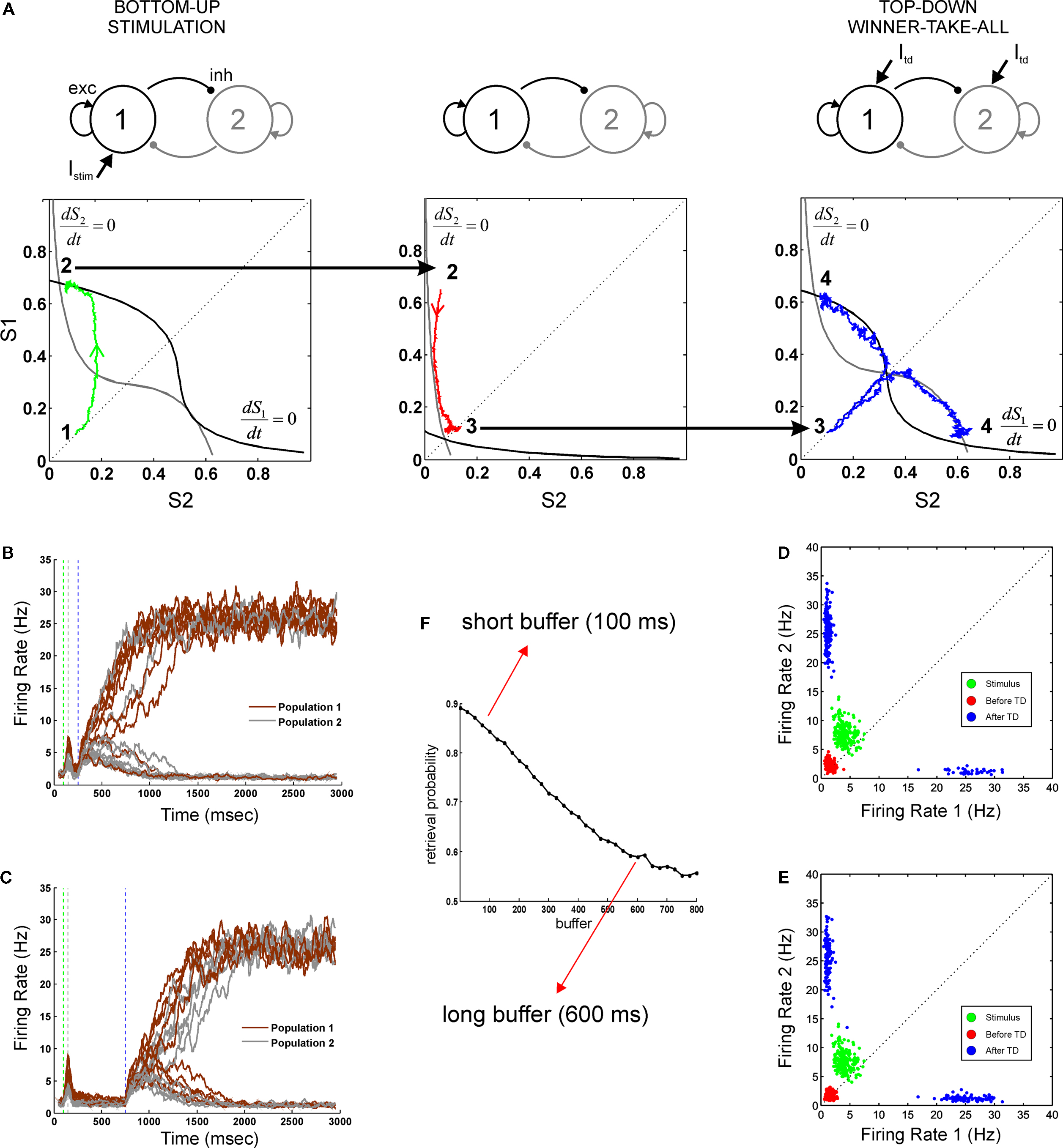
Figure 2. Neural dynamics as a concatenation of discrete processing stages. (A) Sketch of the mean-field architecture and trajectories in phase space. Output synaptic gating variables are plotted against each other. Nullclines for S1 and S2 are plotted in black and grey, respectively. When the stimulus is presented, the system evolves towards the high S1/low S2 asymmetrical attractor. During the buffer, the fixed point in the quiescent state becomes stable and the system evolves towards this fixed point. Top-down control reconfigures the phase space, forcing the system to one of the two high-level attractors. Two trajectories are plotted from the same initial point, giving one correct and one incorrect response. (B,C) Time course of firing rates for short (B) and long (C) buffers. Firing rates are constructed averaging activity over windows of 25 ms, with sliding steps of 5 ms. Red, green, and blue dotted lines indicate load onset, load offset, and retrieval onset, respectively. (D,E) Each processing stage can be understood as a stochastic map in phase space as seen by the distributions of the final states (200 trials) of each processing stage (load, before top-down and after top-down, in green, red and blue, respectively). Each data point indicates the average activity (firing rate) of the last 12.5 ms of the corresponding phase, for short (D) and long (E) buffers. (F) Percent of correct retrievals as a function of the duration of the buffer. Each point is the average over 10,000 trials.
Load
During this phase the two populations receive distinct currents, which represent the sensory inputs evoked by external stimuli. This simulates an experiment in which two stimuli are present at different intensities, or in which only one stimulus differentially activates both populations. The system has two active and stable fixed points with asymmetric basins of attraction (the points in phase-space that will evolve to a fixed point in a fully deterministic system). In the absence of noise, the system will evolve to either S1 or S2 depending solely on whether the initial condition (quiescent S1 and S2) belongs to the basin of attraction of S1 or S2. In the presence of noise, the system has a probability of diffusing (noise-driven fluctuations) across basins of attractions.
Retrieval
During the retrieval period, both populations are stimulated with the same external current which models top-down control. This current is unbiased towards either stimulus. However, it sets the system in a new state that amplifies small current differences. During the retrieval stage, the system has two active and symmetric stable fixed points. The basins of attraction are symmetric and thus the probability of evolving to either of the two fixed points is determined solely by the distance of the initial condition to the diagonal S1 = S2. Following prior convention (Wong and Wang, 2006
), we refer to this important manifold (the line S1 = S2), which divides the phase space, as the decision boundary.
In our simulations, contrary to most previous experiments, both stages will be bracketed in time by a controlled perceptual buffer during which the network does not receive external (top-down or bottom-up) currents. During this stage the system evolves from its current load state towards the quiescent state (∼3 Hz). Any initial condition (resulting from a transient activation) will evolve towards this fixed point. Processing stages are sequentially organized and linked by state continuity: the initial condition of each phase is equal to the final condition of the previous phase.
In this mean-field model with only two active populations, we modeled a stimulus with low visibility by a weak transient response – contrary to the spiking model where we could explicitly model a subliminal presentation by a high contrast stimulus followed by a stimulation of non-specific excitatory cells, which represented the mask. An important aspect of this simplified architecture is that we do not postulate a specific mechanism for the maintenance of the sensory trace. Instead, the loss of the memory trace, results from a passive decay during the buffer towards the quiescent state, which becomes an attractor in the absence of currents. For increasing buffer durations, neural activity will progressively approach the quiescent state – and thus the decision boundary – implying that there is a lesser trace of the sensory memory (Figure 2
A, middle panel).
The three stages of neural activity (transient response – passive fade out – retrieval) are also evident in the time course of the firing rate for both populations (Figures 2
B,C). We measured explicitly the probability of correct retrieval as a function of buffer size and observed that it decreases monotonically until it reaches saturation after about 700 ms (Figure 2
F). The stochastic nature of the decision process can be seen by analyzing the distribution of trials in phase space (Figures 2
D,E). The final state of each stage (load, before retrieval, after retrieval) is represented in a scatter plot (green, red, blue respectively). In this formulation, the entire trial can be seen as a composition of three functions (the load function, the buffer function and the retrieval function) and thus as the concatenation of three operators.
Biophysics of Retrieval Probability and Memory Duration: Neurophysiological Predictions
In a stochastic dynamical system, attractors and noise play opposite roles: stable fix-points result in a shrinking of phase space (all points evolve to the fixed point) while noise diffusion leads to a blurring of phase space. During the buffer, the interplay between these two mechanisms determines the probability of crossing the decision boundary and thus loosing track of the stimulus memory. The probability of stochastically crossing this manifold is determined by the inverse of the coefficient of variation: μ(S1 − S2)/σ(S1 − S2), which essentially estimates the distance to the decision boundary in units of standard deviation. Thus, both the speed of convergence to the quiescent state and the amount of diffusion (noise) determines the duration of the perceptual memory. Some examples are illustrated in Figure 3
A. It is worth remarking that equal values of noise can lead to distributions which appear considerably noisier when the speed of convergence is decreased. In the limit, in which there is no deterministic memory loss (close to the bifurcation value), memory loss is exclusively determined by diffusion (this is close to the situation shown in the lower right panel of Figure 3
A).
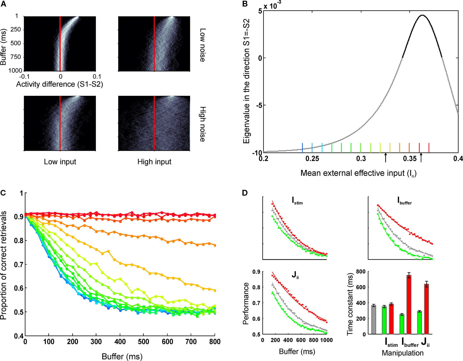
Figure 3. The dynamics of error and correct responses during memory decay and retrieval. (A) We explored the progression of the distance to the decision boundary during the buffer. The four panels represent a factorial exploration of the effects of background current during the buffer [low (left column) and high (right column) input currents] and the noise level [low (top panels) and high noise (bottom panels)]. Within each panel, each line represents a histogram, coded in a grey color code. The y-axis indicates buffer time and the x-axis indicates the difference in activity between S1 and S2. In all panels it can be seen that in the beginning of the buffer activity is clustered in a value of (S1 − S2) (the initial condition had no dispersion) and as time passes (going down in the y-axis) the distribution probability approaches the decision boundary and becomes wider. (B) The speed of convergence to the decision boundary can be estimated by calculating the eigenvalue of the quiescent fix point in the linearized system as a function of the background input currents. For high background currents – just bellow the bifurcation – speeds are arbitrarily slow (stimulus memory is lost by noise diffusion). For lower currents, the speed increases (in absolute value) reaching an asymptote which establishes a maximal rate of convergence and thus a minimal temporal decay constant. This critical time is determined by the NMDA temporal constant and determines that perceptual buffers last at least about 100 ms. The current values which correspond to the retrieval mode (positive eigenvalue) are indicated in bold. Black arrows indicate the default values used as background currents during buffer (I0 = 0.3255 nA) and retrieval (I0 = 0.3619 nA) throughout the paper. (C) Simulations of a sensory retrieval experiment using the original (non-linear) system of equations, varying the duration of the buffer and the background current during the buffer. Information is lost exponentially with a time constant which increases with increasing currents and has a lower bound. Each curve is the average over 5,000 trials. Each color represents a different input value, as indicated in Figure 2
B. Values range from 0.24 to 0.37 nA, in intervals of 0.01 nA. (D) Effect of different parameter manipulations on task performance: stimulus intensity (Istim, upper left panel), top-down currents during the buffer (Ibuffer, upper-right panel), and recurrent strength (Jii, lower left panel). The baseline (same as data in Figure 2
F) is plotted in gray. Higher values are plotted in red and lower values in green. Data is fitted with exponential distributions. Error bars indicate 95% confidence bounds.
A quantitative analysis of these dependencies can be understood analyzing the comparatively simpler linearized system of equations (Strogatz, 1994
). In a linear system, the dynamics can be collapsed to a single number – referred as the eigenvalue – which indicates the speed of convergence to the fixed point. Thus, to explore the effect of different biophysical parameters in the duration of sensory memory, we calculated the eigenvalue of the quiescent fix point in the direction orthogonal to the decision boundary (S1 = −S2, Figure 3
B).
A current discussion in the literature has debated whether top down control is allocated sequentially in an all or none fashion to distinct processors or rather, whether certain amount of top-down control can be shared among concurrent processes. In our simplified network each population receives a single current type (i.e. different inputs do not target distinct receptors or synapses with different dynamics) and thus all input currents are additive. Thus, to understand the effect of sub-threshold modulations (i.e. for which the only active state is quiescent) on the dynamics of sensory memory, we gradually increased the background currents during the buffer from the default values to the bifurcation point in which the network switches to a retrieval mode (Figures 3
B,C).
The simulations resulted in the following conclusions:
1. For small background current values the eigenvalue is negative indicating that the default state is an attractor. At a certain critical value of the top-down current the eigenvalue becomes positive. This merely reflects that the network undergoes a bifurcation in which the quiescent state is not stable anymore and switches to a retrieval operational mode.
2. For high background currents within the buffer regime – just bellow the bifurcation point – speeds of convergence to the decision boundary is close to zero, indicating that stimulus memory is lost only by noise-driven drift.
3. As the background currents decreases, the speed of convergence increases monotonically (the eigenvalue becomes more negative). This process reaches an asymptote which establishes a maximal speed of convergence, or, conversely, a minimal temporal decay constant. This critical time is established by the NMDA temporal constant and determines that the system cannot relax (at least passively) faster than about 100 ms.
Based on these observations, we simulated a sensory retrieval experiment, using the full (non-linear) system of equations while varying the background current during the buffer (Figure 3
C). As suggested by the lineal analysis, information is lost exponentially with a time constant which decreases monotonically with decreasing background current, reaching a lower bound (green to cyan curves result in almost identical temporal decay functions, although the background current is lowered). Thus, variations in top-down control – even at modest levels which are insufficient to achieve amplification – affect the time constant of the decay of the experimental buffer establishing a concrete prediction which can be submitted to experimental verification.
Next, we wanted to investigate whether other biophysical and experimental manipulations changed the time course of the perceptual memory (Figure 3
D). We performed three simulations changing the background current during the buffer phase (which from prior results we know it affects the temporal constant), the strength of recurrent connections and the strength of the stimulus. While overall all manipulations affected the probability of correct retrieval, they had a different impact in the dynamics of the memory trace. The background current and the strength of recurrent connections (which is also a plausible biophysical model of top down control – see Discussion) affected the temporal constant of the exponential (for recurrent strength JN11 = [0.24, 0.207] nA, the temporal constants for the best-fit exponentials (R2 > 0.994) were τ = [289, 636] ms, and for buffer currents Ibuffer = [+15, −15] Hz, the temporal constants were τ = [250, 750] ms, respectively). On the contrary, changing the stimulus strength affected the gain of the perceptual buffer (a multiplicative effect in the exponential), with no effect in its temporal constant (τ = [351, 383] ms for I1 = [91.2, 100.8] Hz respectively).
From Biophysics to Behavior: Performance of the Model In A Dual-Task Experiment
As discussed in the introduction, there are not (to our knowledge) single-cell neurophysiological experiments which have investigated explicitly and in a controlled manner the temporal bracketing between sensory stimulation and top-down control. On the contrary, many variants of this experiment – as for instance in the AB and the Partial Report Paradigm have been largely explored in the experimental psychology literature (Raymond et al., 1992
; Sperling, 1960
).
In the AB, two masked stimuli in rapid succession have to be reported (Figure 4
A); the second stimulus is often missed, and the probability of not seeing the stimulus is a function of the SOA. Despite its conceptual simplicity, an extensive exploration of this phenomenon has revealed a quite complex description (see Discussion and, for instance, Bowman and Wyble, 2007
for an extensive review). The aim of this work is not to provide a model which will account for this rich diversity of observations. Rather, we show that the simple biophysical architecture described in this paper can account for one factor which is common to these distinct behavioral experiments: the exponential decay of information.
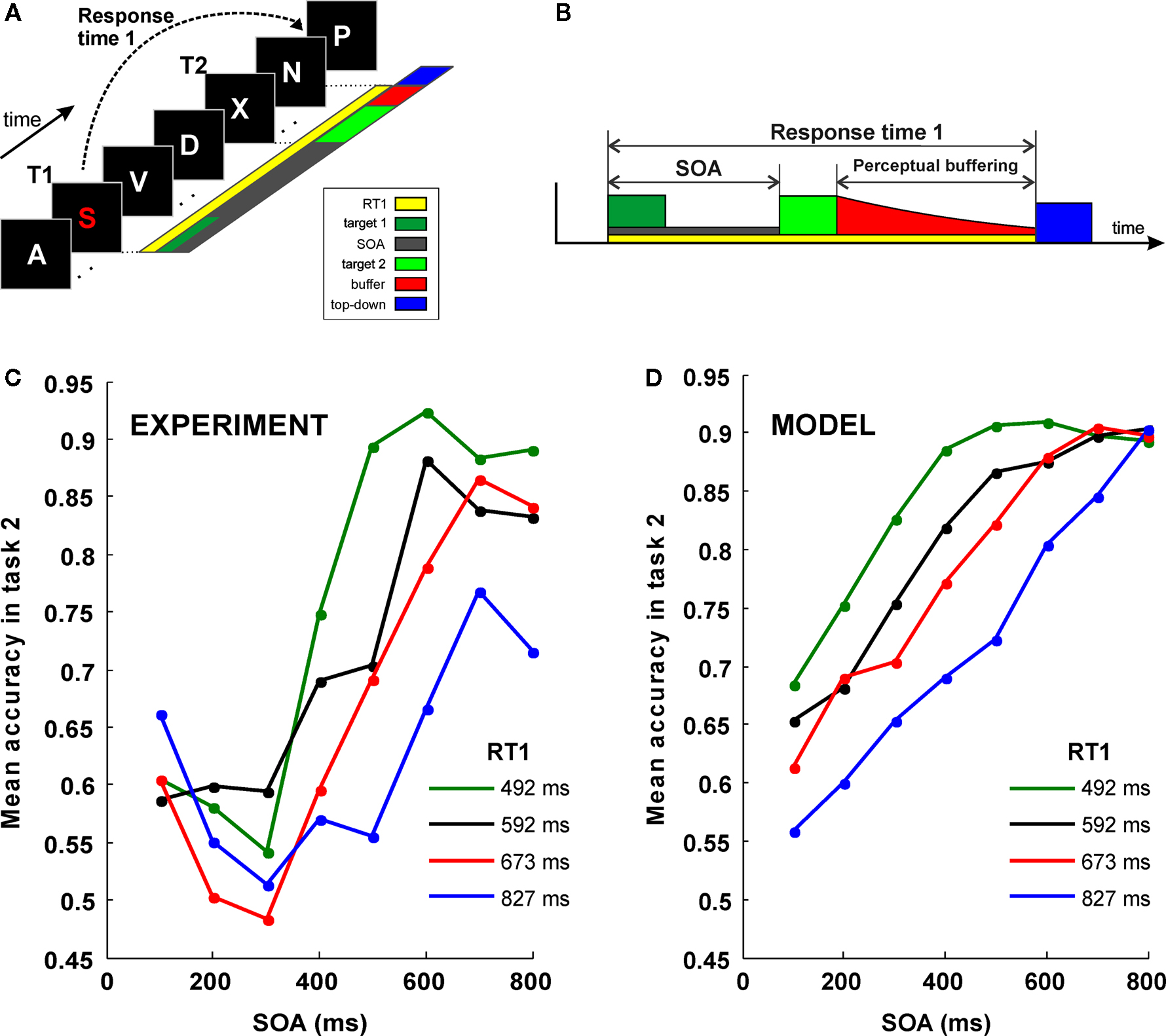
Figure 4. Simulation of a dual-task interference experiment. (A) Sketch of the “speeded attentional blink” paradigm used by Jolicoeur (1999)
: letters are presented in rapid serial visual presentation (RSVP), each letter presented for 100 ms with no blank ISI. Subject must report both T1 and T2. T1 must be reported as soon as possible, while T2 is reported at the end of the trial, without time pressure. SOA is systematically varied in order to study its effect on T2 accuracy. (B) A schematic model of interference based on sequential top-down allocation. Top-down allocation to T2 can only occur once it has been released from T1 and thus the duration of the sensory buffer is determined by RT1 − SOA − P. (C) Mean accuracy in task 2 for different SOA, as obtained by (Jolicoeur, 1999
). The proportion of trials where T2 was correctly identified (given T1 correct) is plotted against SOA (in milliseconds). Results are grouped in four categories according to the response time to the first task (RT1). Mean RT1 is indicated. (D) Result of the simulations of the model after averaging 1,000 trials for each condition.
In the AB, it has been shown that the probability of seeing the second target is also a function of the response time to the first task (RT1) (Jolicoeur, 1999
) (Figure 4
C). This result can be interpreted in terms of a very simple theoretical scheme, according to which, top-down control is sequentially allocated to both tasks. According to this interpretation, top-down control to T2 is only delivered once it has been released from T1 and thus the longer the time to complete the first task (RT1) the larger the gap between the presentation of T2 stimulus and the allocation of top-down control (see Figure 4
B for a simple illustration of the scheme).
More precisely, following the assumptions of a sequential deployment of top-down control, the duration of the perceptual buffer can be obtained from experimental observables: as sketched in Figure 4
B, the duration of the perceptual buffer of S2 is determined by:

where P is a fixed value determined by the latency of the sensory response (Pashler, 1994
; Sternberg, 1969
).
We modeled an extremely simplified version of T2 processing in this AB experiment, using the reduced two-dimensional network, with the same set of parameters as in Figure 2
.
For each RT1 and SOA values we calculated the duration of the buffer following Eq. 1. We then simulated 10,000 trials, following exactly the procedure of Figure 2
(i.e. a stimulus presentation of 50 ms biased to one of the selective populations) – followed by a buffer in which the background current was set to 0.3255 nA and then a retrieval period. In each trial, the response was considered correct if the activated population after retrieval corresponded to the more stimulated population. We then averaged, for each SOA and RT1 value, the percent of correct responses for comparison with the experimental results. Note that here we are not simulating the processing of T1 and the precise gating mechanisms that control the shifting of attention between T1 and T2. A full simulation of the dynamics of the engagement and disengagement of top-down control during the processing of multiple sensory elements will be an objective for future studies. Rather, we make the simple assumptions that: (1) top-down to T2 is directed after the conclusion of the first task, (2) that this is indexed by RT1 and (3) that top-down control is implemented by a non-specific current to the network which sets it in a retrieval mode.
The experiments show that this single parameter derived from SOA and RT1 (the duration of the sensory buffer), is capable of capturing one of the main qualitative aspects of the dependence of performance with RT1 and SOA (Figures 4
C,D), which captures most of the variability for intermediate SOA values. The observations for very short and for very long SOA values cannot be explained by a passive decay of information mechanism. For instance, this over simplified model predicts that performance is worse at the shortest SOA values and an asymptotic performance for large SOA values which is independent of RT1. These predictions are in contradiction with the observations and thus pose a limit on which observations can be explained simply by passive decay of information.
A more direct experimental psychological demonstration of the memory decay during the interval between stimulus presentation and top-down control comes from partial report experiments (Sperling, 1960
). In these experiments, participants are asked to recall only a portion of the stimulus array. Performance in many different variants of this experimental design has been shown to decay exponentially with the inter-stimulus interval (ISI), the time between the presentation of the stimulus and the spatial cue indicating the item to report (Loftus et al., 1992
; Sperling, 1960
).
Here we modelled an experiment in which eight different letters appeared simultaneously for 106 ms, arranged on a circle around the fixation point. A cue was then presented at variable ISI values, ranging from 24 to 1,000 ms, after the offset of the array display (Figure 5
A) (Graziano and Sigman, 2008
).

Figure 5. Simulation of a partial report experiment. (A) Sketch of the partial report experiment (Graziano and Sigman, 2008
). Eight letters appeared simultaneously for 106 ms on a computer screen, arranged on a circle (5.5°) around the fixation point. Each letter was presented in uppercases and chosen at random from a set of 26 letters. Trials started with a fixation point at the center of the display. After 1,000 ms, the array of eight letters was shown for 106 ms. After removal of the array of letters participants were cued with a color marker at the location of the letter that had to be reported. The cue was maintained on the screen until participants made a forced choice. Eight target-cue asynchronies (ISI) were investigated: the cue appeared 24, 71, 129, 200, 306, 506, 753, 1,000 ms after the offset of the array display. (B) Description of the network and of the model. Each letter is represented by a variable with a normalized output in the range (0, 1). For simplicity, we neglect any interaction between letters in different positions of the stimulus array and thus the eight different locations are modeled independently. The network is endowed with local excitatory connection – each excitatory population connects to one inhibitory population – and global inhibition – each inhibitory population projects uniformly to all excitatory populations. The number of active populations in the stable state decreases with the inverse of inhibition strength and increases with top-down strength. This dependency assures that a wide range of parameters exists for which the network is set in a winner-take-all mode (i.e. retrieves a single population). In each location, only one population receives bottom-up input during stimulus presentation (green populations in the lower-left panel). During retrieval, all excitatory populations receive equal top-down currents (blue populations in the lower-right panel). (C) Transient responses to the stimuli and top-down amplification at the target location. In each position, the activity of the 26 possible responses (letters) is plotted. Top-down current sets a winner-take-all competition at target location, where the initial transient response biases the competition towards the presented letter. Stimulus onset, stimulus offset, and cue onset are marked with green, red and blue lines respectively. (D) Performance for human subjects (red dots) and model (black line). Solid curve was obtained by fitting model simulations to an exponential distribution (R2 > 0.995). Data for the fit was obtained by averaging 3,000 simulations at each of 43 inter-stimulus-cue intervals (from 0 to 1,050 ms at intervals of 25 ms).
In the AB experiment, as in most simple-decision experiments, subjects (and the models) perform a binary choice. On the contrary, in the partial report experiment the number of possible responses corresponds to the 26 letters of the alphabet. Thus the model described earlier (Figure 2
) was extended to 26 different excitatory populations. In addition to all letter identities, the network has to code the position of the array. For simplicity, all spatial locations were modeled independently, i.e. there were no direct connections between populations coding for different locations (Figure 5
B). Within each location, populations responding to distinct letters were arranged on a circle and connected to the two closest neighbors. These connections resulted in partial spreading of activity and, in future work, should permit exploring the confusion effect in iconic memory experiments (i.e. when the letter F is responded when the letter E was present in the cued location). For the modeling of the main factor, the exponential decay in performance, these connections were unnecessary and removing them yields essentially the same results.
On the contrary, the topology of the inhibitory network played a critical role in the model. As shown in Figure 5
B, inhibitory neurons receive synaptic inputs from a single excitatory population and then project globally to all excitatory populations. Local excitation and global inhibition has been assumed as a plausible architecture in many computational and theoretical studies (Ardid et al., 2007
; Compte et al., 2000
; Ermentrout, 1992
; Kang et al., 2003
; Wang and Terman, 1995
). This asymmetry (local presynaptic and global postsynaptic connections of inhibitory neurons) turned out to be critical to assure that the network scaled correctly and generated a winner-take-all behavior during retrieval. This can be intuitively understood with a simple qualitative calculation involving the balance of currents in excitatory populations and assuming that populations fire following a step function, if the input current is larger than a threshold T. Each excitatory population receives input currents:

Which respectively correspond to: (1) self-excitation (2) an external excitatory current which captures the background and top-down currents and (3) inhibitory inputs. If the population is active and ISE + IE − IINH > T, it will stay active. Of course, this algebraic equation needs to be iterated dynamically since once the population is active it changes the inputs to other populations, which in turn change the input to others populations and so on. However, without need of solving this differential equation it can be understood that if ISE + IE − IINH > T (i.e. the active population keeps on firing) and IE − IINH < T (i.e. the silent populations stay silent) then the network configuration with a single active population is stable.
This consideration is general and does not make assumptions about the architecture of the network. The important aspect of the proposed architecture is that inhibition to all neurons increases linearly with the number of excited neurons and thus the balance between inhibition and excitation can be easily controlled. For this architecture the input current to a excitatory population becomes:

where we have simply replaced from Eq. 2 the inhibition current by a constant (the efficacy of synaptic inhibition) multiplied by the number of active populations (recall that the key aspect of this architecture is that for each active excitatory population, there is one active inhibitory population). It is easy to see that, for fixed values of IE and T, there is a critical number of excited populations (NC) such that:

In this case, and if silent excitatory populations stay silent which can be assured if

a stable state with NC neurons exists. Note from Eq. 4 that the stable state with maximal number of active populations can be related to μ by:

We verified this relation (Figure 5
B), showing that NC decays as 1/μ, with a constant that depends on the excitatory input. Note that this dependence implies that there is a wide region in parameter space for which there will be a winner-take-all (i.e. a single active population, NC = 1). Thus, we could easily adjust the parameters, in a stable manner to set the network in a mode in which there is passive decay during the buffer and amplification to a single response after allocation of top-down control currents. It is interesting that in Iconic Memory Experiments subjects often retrieve more than one letter with very high confidence. Thus, in future experiments and model it might be worth exploring the number of elements which can be correctly retrieved in iconic memory experiments and how this may relates in a more quantitative manner to the architecture of inhibition in recurrent memory networks.
Once we could assure a stable winner-take-all network for a large number of excitatory populations, we proceeded to explore whether retrieval in this network showed an exponential dependence with ISI, as observed in the experiments. We simulated the dynamics of the network, 3,000 trials for each ISI condition (Figures 5
C,D). Figure 5
C shows the dynamics of all populations in a representative trial. The stimulus was modeled as a constant input current, lasting 100 ms to one of the populations in each spatial location. The stimulated population at each location evoked a large transient response which decayed to the quiescent state. Top-down was directed to the cued location of the visual field at a fixed delay (set at 200 ms) following the cue. The delay between the cue and the onset of top-down modulation – which was necessary to explain performance level bellow 100% for the shortest ISI values – has been found in different experimental setups (Bisley and Goldberg, 2006
; Lamme, 1995
; Li et al., 2006
; Roelfsema et al., 1998
).
The performance of these simulations for long ISIs is at chance level (which here is 1/26) since the transient response has completely decayed. This is in contradiction with the results of iconic memory experiments – in which it is observed that the asymptotic performance is significantly above chance – and we hypothesized that this is due to the fact that spontaneously (before the beginning of the trial) top-down control is directed to a window of the visual scene which covers a fraction of the display. We assumed that in trials in which the cued letter was within the attended window, performance was perfect. In trials in which the cued location was outside of the attended window, top-down control is directed to this location only after the presentation of the cue, and performance can be estimated by the model. This simply results in a linear correction of the probability of correct performance, as described in the “Materials and Methods” section.
As with the simulation of the AB experiment, this aims to explain a complex psychophysical experiment in an admittedly simplified simulation. Future work should address the spontaneous allocation of top-down control and the subsequent shifting to other cued location in a full simulation which incorporates in the network the dynamics of these processes. Here, we merely show that: (1) correct retrieval after passive delay accounts for the correct scaling observed in psychophysical experiments and (2) that a recurrent network can be configured to elicits passive decay of information in absence of top-down control and switch, with the allocation of top-down control, to a winter-take-all configuration for a large number of distinct excitatory populations.
In this work we have attempted to unite, through a simple biophysical implementation, two different literatures which have independently investigated the dynamics of top-down control. Single single-cell monkey electrophysiology have investigated in detail the distinct waves of responses to a sensory stimulus in situations of varied ethological relevance, without explicitly manipulating the temporal gap between sensory stimulation and top-down control. Different behavioral paradigms which include the PRP (Pashler, 1994
; Smith, 1967
; Telford, 1931
), the AB (Raymond et al., 1992
) and partial report experiments (Sperling, 1960
) have investigated performance (visibility, ability to respond to an item, etc…) in experiments in which an interference probe perturbed the ability to timely attend to a presented stimulus, leading to experiments in which the gap between sensory stimulation and top-down control is presumably controlled experimentally but in which this relation can only be made indirectly.
We presented a biophysical model intended to bridge the partial retrieval of sensory information – as determined in partial report and AB experiments – to the two-stage organization of responses in visual areas of awake-behaving monkeys. We show that a simple model, involving a first initial transient response followed by a forced competition set out by top-down currents can account for the partial retrieval of sensory information observed in partial report and AB experiments. The proposed model can successfully explain functional dependencies of interference experiments, such as the visibility of a target as a function of the time it takes to report a previous item and the rapid memory loss of a stimulus display.
The model works by concatenation of discrete processing stages, determined by specific stimulus and top-down context. Contrary to “boxological” models, where different functions are generally assigned to different areas in the brain, in our model the same network performs the different processing stages. The particular configuration of external inputs (stimulus and top-down) sets the circuit in a specific working mode, which can respond transiently, decay or amplify information. Our model suggests that the “memory” of a stimulus resides in the decaying trace of a stimulus transient response and the speed of this decay depends on the background current and recurrent connection strength, but not on the stimulus intensity. The model does not need to assume an active process in the maintenance of iconic memory, establishing a qualitatively different form of persistence than working memory models in which the memory is actively held in a reverberation process. In accordance with this distinction, experimental results have shown that iconic memory decays much more rapidly than working memory (in a few hundred milliseconds) and is labile, i.e. can be destroyed by the presence of a concurrent stimulus. Previous fMRI studies in a partial report experiment have also suggested a passive role of iconic memory, by showing that activity in the visual cortex is identically amplified when the cue is presented 200 ms before or after the stimulus presentation (Ruff et al., 2007
).
A similar observation comes from a classical demonstration of dual-task interference, the PRP. In this experimental setup in which two targets have to be responded rapidly, if the second processed target is not masked it can be retrieved correctly with virtually perfect performance. There is, however, a very clear trace of interference as reflected in the fact that the second target is only responded after a delay (Pashler and Johnston, 1989
). Two principal observations suggest that the nature of this memory is qualitatively different from working memory and similar to the iconic memory observed in partial report paradigm experiments: (1) this memory is labile (i.e. a brief mask is sufficient to degrade it) as shown in the behavioral experiments by Jolicoeur and colleagues, reported in this paper and (2) functional imaging experiments have not shown any activation related to the maintenance of the second target while the first task is being executed (Dux et al., 2006
; Jiang et al., 2004
; Sigman and Dehaene, 2008
). Thus, the physiological nature of the memory of the delayed stimulus, which does not seem to involve an active process, constitutes an open question suitable for theoretical and computational investigation. Here we showed that a passive decay memory, sustained in the convergence to a quiescent state in the absence of top-down control can account for these principal observations. Another possible physiological alternative, which may explain the lack of a correlate of this memory in fMRI experiments, involves low metabolic-cost synaptic memories (Mongillo et al., 2008
).
Duration of Sensory Information, from Biophysics To Psychophysics
Our explorations have shown that two factors control the duration of iconic memory, a uniform background current and the strength of recursive connections. While in our model we have investigated the effect of varying these parameters in a simple model of a processing network, an interesting possibility is that these parameters may vary at different stages of the cortex. For instance, the size of the receptive fields increase as one proceeds in the visual hierarchy (Rolls, 2000
), indicating a larger population of neurons with similar response properties and thus stronger effective recurrent connections. It is thus possible and a matter for further experiments to investigate whether, the sensory memory, i.e. the duration of a transient response evoked by a stimulus, may increase (even in the absence of conscious perception) as one progresses from primary sensory areas to the frontal cortex. Another possibility is that, within the same cortical region, effective recurrent strengths may be changed by top-down control. While no direct biophysical evidence of such mechanism exists, this possibility is suggested by indirect evidence which has shown that top-down influences target specifically contextual and integrative properties of V1 neurons (Gilbert and Sigman, 2007
; Li et al., 2004
, 2006
). Indeed, we performed simulations in which the retrieval stage – when information is amplified under top-down control – is modeled by an increase of the recurrent connections (instead of increasing the background currents) which yielded virtual identical results as the ones described in the paper.
A theoretical debate has been held on whether, in dual-task experiments, top-down allocation is a sequential all-or-none process or whether it can be distributed in a graded manner across different processes (Shapiro et al., 2006
; Tombu and Jolicoeur, 2003
, 2005
). Our model suggests an experimental approach to discern between these alternatives. If top-down control is partially allocated to the task which is not consciously being executed – even at modest levels which are insufficient to achieve amplification – it should affect the time constant of the decay of the experimental buffer. Indeed, some experiments have investigated which parameters can affect the persistence of a stimulus of iconic memory, measuring quantitatively the temporal constant of the memory decay in partial report paradigms. Our model shows that different factors map to distinct parameters of the exponential decay. For instance changing the background current during the buffer affects the temporal constant, while increasing stimulus strength affects the exponential decay function in a multiplicative manner. Thus, the model predicts that different experimental manipulations should be found affecting distinct parameters of the iconic memory decay. Previous experiments provide partial evidence in support of this view. For instance, iconic memory decays much faster for observers with Mild Cognitive Disorders than for normal controls even when they performed at equivalent levels assays of visibility and of short-term memory (Lu et al., 2005
). Our model predicts that the temporal constant of the memory decay can be affected independently of stimulus strength and suggests that the patients’ deficit may be explained by a reduced capacity to maintain low levels of top-down control during the buffer. Complementarily, in a partial report experiment which studied the duration of the iconic memory as a function of different geometric and spatial factors, we found that letter frequency affects the memory decay in a multiplicative manner, without changing the temporal constant (Graziano and Sigman, 2008
). This is precisely the prediction of our model, given that more frequent letters elicit stronger average response than non-frequent letters in occipito-temporal visual cortex (Vinckier et al., 2007
).
Relation to Other Models of Dynamics of Neural Activity
At this stage, our model does not intend to provide a full explanation of the dynamics of sensory processing and top-down control. Rather we used the proposed model as a tool to explain and interpret observations in different experiments. We suggest that observations from partial report paradigm and the AB may involve a common mechanism. Our model, although admittedly oversimplified, establishes concrete predictions which may guide future neurophysiological experiments.
More detailed models of the AB (Bowman and Wyble, 2007
; Dehaene et al., 2003
; Fragopanagos et al., 2005
; Nieuwenhuis et al., 2005
) can capture some elements which our simple model is unable to describe. For instance, it can’t explain why in the AB performance increases for very short SOA. This effect, known as lag-1 sparing, is still largely unexplained (Dell’Acqua et al., 2007
) and has been attributed to mechanisms beyond the present model, such as an attentional “blaster” effect on selected target stimuli (Bowman and Wyble, 2007
). It is clear that our minimal model cannot account for this effect, since shorter SOA result in longer buffers and thus worse performance. Another aspect that cannot be accounted by our simple model is the effect of RT1 when SOA is large. In the model, if SOA > RT1 − P, the buffer duration is zero and the processing of T2 is independent of RT1. Experimental results show that performance does recover as SOA increases, but this recovery is not as complete as predicted by our model. This may be due to the presence, in actual experiments, of a small fraction of trials at long RT1 in which the subject is distracted and fails to reallocate attention to the second stimulus.
Numerous efforts have been made to generate biophysical models which account for important elements of cognition, such as, Bayesian inference in sensory perception (Knill and Pouget, 2004
; Pouget et al., 2003
), information maintenance in working memory (Brunel and Wang, 2001
; Durstewitz et al., 2000
), attentional modulation (Ardid et al., 2007
; Deco and Rolls, 2003
), decision-making (Lo and Wang, 2006
; Machens et al., 2005
) and conscious access (Dehaene et al., 2003
; Izhikevich and Edelman, 2008
). Mean-field approximations have been used to reduce the dimensionality of large-scale spiking models as well as to get a geometric understanding of their behavior (Brunel and Wang, 2001
; Renart et al., 2004
; Tovee et al., 1993
). This paper has been motivated by this strategy of generating simple dynamic models from large-scale architectonic models, to address an important aspect of information flow: the persistence of sensory buffers. As described in other previous models (Dehaene et al., 2003
), only a fraction of sensory information is amplified and piped to the decision-making or the motor system. Here we have incorporated the dynamics of the unattended and the to-be-attended stimuli. Our model was able to capture different experimental observations and led to the following predictions:
1. Both buffering and retrieval can occur within sensory areas initially involved in the feed-forward response to the stimulus, without the need to postulate specific “buffer areas”.
2. Firing rates just prior to top-down signals for retrieval are a predictor of the probability of correct retrieval.
3. Mean activity in sensory areas decays almost exponentially during the delay period, and this decay accounts for the memory loss. There is an upper limit to the speed of this decay, determined by NMDA receptors. Pharmacological blockage of these receptors should significantly reduce the temporal constant of the decay.
4. In behavioral experiments, blocking NMDA receptors should result in the inability to retrieve unattended stimuli, as can be explored with a partial report paradigm experiment in animal models.
5. In a partial report experiment in which attention is removed away from the presented letter (for instance with a competing task in the fovea as done in (Joseph et al., 1997
)) iconic memory should decay very fast (but with unaffected amplitude). This prediction is parametric; the exponential time constant should decrease monotonically with the amount of attention deployed to the competing task. Moreover, if top-down resources are completely allocated away from the partial report paradigm task, the asymptotic performance for very long ISI should be at chance levels.
6. We predict that this observation should co-vary with the temporal constant of populations of neurons in sensory areas.
7. If increased receptive field size determines stronger local recurrence between excitatory populations, the temporal constant of the decay of stimulus information should increase as one proceeds in the visual hierarchy.
The authors declare that the research was conducted in the absence of any commercial or financial relationships that could be construed as a potential conflict of interest.
We thank Stefano Fusi, Kong-Fatt Wong, Xiao-Jing Wang and Gustavo Deco for sharing the computer code. This work was partly supported by grants from SECYT (PICT 38366) and Peruilh Foundation, and by the Human Frontiers Science Program.