1
Network Dynamics Group, Max Planck Institute for Dynamics and Self-Organization, Göttingen, Germany
2
Bernstein Center for Computational Neuroscience, Göttingen, Germany
3
Center for Brain Science, Faculty of Arts and Sciences, Harvard University, Cambridge, MA, USA
Large sparse circuits of spiking neurons exhibit a balanced state of highly irregular activity under a wide range of conditions. It occurs likewise in sparsely connected random networks that receive excitatory external inputs and recurrent inhibition as well as in networks with mixed recurrent inhibition and excitation. Here we analytically investigate this irregular dynamics in finite networks keeping track of all individual spike times and the identities of individual neurons. For delayed, purely inhibitory interactions we show that the irregular dynamics is not chaotic but stable. Moreover, we demonstrate that after long transients the dynamics converges towards periodic orbits and that every generic periodic orbit of these dynamical systems is stable. We investigate the collective irregular dynamics upon increasing the time scale of synaptic responses and upon iteratively replacing inhibitory by excitatory interactions. Whereas for small and moderate time scales as well as for few excitatory interactions, the dynamics stays stable, there is a smooth transition to chaos if the synaptic response becomes sufficiently slow (even in purely inhibitory networks) or the number of excitatory interactions becomes too large. These results indicate that chaotic and stable dynamics are equally capable of generating the irregular neuronal activity. More generally, chaos apparently is not essential for generating the high irregularity of balanced activity, and we suggest that a mechanism different from chaos and stochasticity significantly contributes to irregular activity in cortical circuits.
Most neurons in the brain communicate by emitting and receiving electrical pulses, called action potentials or spikes, via chemically operating synaptic connections. Local cortical circuits often exhibit spiking dynamics that is highly irregular and appears as if it were random. Such irregular activity at low neuronal firing rate is thus considered a basic “ground state”. It is characterized by individual neurons that display largely fluctuating membrane potentials and highly variable inter-spike-intervals (ISIs) as well as by low correlations between the neurons (v.Vreeswijk and Sompolinsky, 1996
, 1998
; Brunel, 2000
; Vogels and Abbott, 2005
; Kumar et al., 2007
). Originally, this dynamical state seemed to be in contradiction to cortical anatomy, where each neuron receives a huge number of synapses, typically 103–104 (Braitenberg and Schüz, 1998
): One might expect that a large number of uncorrelated, or weakly correlated synaptic inputs to one neuron, given the central limit theorem, sums up to a regular total input signal with only small relative fluctuations, therefore excluding the emergence of irregular dynamics. So the finding of highly irregular activity might be surprising.
This issue was resolved by the idea of a “balanced state” (v.Vreeswijk and Sompolinsky, 1996
), in which excitatory (positive) and inhibitory (negative) input balances such that the average membrane potential is sub-threshold and strong fluctuations once in a while are sufficiently depolarizing to initiate a spike. The original work “Chaos in neuronal networks with balanced excitatory and inhibitory activity” (v.Vreeswijk and Sompolinsky, 1996
) was an analysis of a self-consistent, highly irregular “balanced” activity for sparse random networks of binary model neurons. It was shown that the balanced state naturally and robustly occurs in large networks if the inhibitory and excitatory coupling strengths and their respective numbers of synapses appropriately scale with each other. Moreover, flipping the state of only one of the binary neurons in a large network (i.e. applying the smallest possible non-zero perturbation in such a system) leads to a supra-exponential divergence between the perturbed and the unperturbed realizations of the network dynamics, exemplifying the extremely chaotic nature of the balanced activity (v.Vreeswijk and Sompolinsky, 1996
, 1998
).
Later analysis (Amit and Brunel, 1997
; Brunel, 2000
) of networks of integrate-and-fire neurons demonstrated that the mean field description of the balanced activity for these continuous-state neuron networks is very similar to that of the original binary neuron networks. These and related results (Amit and Brunel, 1997
; Brunel, 2000
; Timme et al., 2002
; Timme and Wolf, 2008
) indicate that statistically the same balanced activity persists both in networks with external excitatory inputs and recurrent inhibition only as well as in networks with equal total amounts of recurrent inhibition and recurrent excitation. Given these findings about the robustness of the balanced state, the original work (v.Vreeswijk and Sompolinsky, 1996
, 1998
) together with common intuition may suggest that highly irregular activity originates from chaotic network dynamics. This hypothesis, however, has not been systematically investigated so far. Recent research even points towards the contrary: it shows that in globally coupled networks without delay the dynamics tends to converge to stable periodic orbits if inhibition dominates (Jin, 2002
). Numerical investigations of weakly diluted inhibitorily coupled networks without delay show that although the dynamics may be irregular, its Lyapunov exponent is negative (Zillmer et al., 2006
). These numerical simulations also demonstrate by example that the dynamics converges to a periodic orbit after long quasi-stationary transients. Interestingly, a related article (Zillmer et al., 2009
) also gives numerical evidence that there can be chaos and long transients even in networks with only inhibitory connections.
In this article we show analytically in the limit of fast synaptic response, that in inhibitory networks with inhomogeneous delay distribution and arbitrary, strongly connected topology (A network is strongly connected if there is a directed path of connections between any ordered pair of neurons.) any generic trajectory is asymptotically stable. After a (typically long) stable transient characterized by irregular activity the dynamics converges to a periodic orbit that is also stable, in agreement with the results presented by Memmesheimer and Timme (2006a) and Timme and Wolf (2008)
. In particular the transients are not chaotic in contrast to the ones occurring in purely excitatorily coupled networks (Zumdieck et al., 2004
). We show that this collective dynamics is robust upon increasing the synaptic response time from zero and upon replacing some inhibitory by excitatory interactions. Nevertheless, if the synaptic response becomes too slow or the number of excitatory interaction too large, the collective dynamics becomes chaotic via a transition where the Lyapunov exponent changes smoothly and the spiking activity stays highly irregular. Thus the irregularity equally prevails in networks with stable as well as in networks with chaotic dynamics (Figure 1
), leaving no evidence that chaos generates the irregularity.
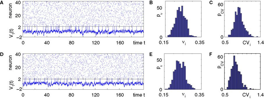
Figure 1. Highly irregular spiking activity equally emerges from chaotic and from stable circuit dynamics. Irregular dynamics in purely inhibitorily (A-C) and inhibitorily and excitatorily (D–F) coupled random networks of identical leaky integrate-and-fire neurons (N = 400, γi ≡ 1, VΘ,i ≡ 1,  |Pre(i)| ≡ 80). (A,D) Spiking dynamics (A)
  Ii ≡ 4, NE = 0; (D)
  , NE = 10000, where the NE excitatory couplings are distributed such that each neuron has the same number of excitatory inputs. The upper panel displays the spiking times (blue lines) of the first 40 neurons. The lower panel displays the membrane potential trajectory of neuron i = 1 (spikes of height ΔV = 1 added at firing times). (B,E) Histogram of mean firing rates νi. (C,F) Histogram of the coefficients of variation CVi:= σi/μi;
 averaged over time.
|Pre(i)| ≡ 80). (A,D) Spiking dynamics (A) Ii ≡ 4, NE = 0; (D) , NE = 10000, where the NE excitatory couplings are distributed such that each neuron has the same number of excitatory inputs. The upper panel displays the spiking times (blue lines) of the first 40 neurons. The lower panel displays the membrane potential trajectory of neuron i = 1 (spikes of height ΔV = 1 added at firing times). (B,E) Histogram of mean firing rates νi. (C,F) Histogram of the coefficients of variation CVi:= σi/μi; averaged over time.Some analytically accessible aspects of the stable irregular dynamics have been briefly reported before (Jahnke et al., 2008a
). Parts of this work have been presented by Memmesheimer (2007) and at a Bernstein Symposium (Jahnke et al., 2008b
).
We consider networks of N neurons with directed couplings that interact by sending and receiving spikes. If such a directed connection exists from neuron j to neuron i, we call i postsynaptic to neuron j. We denote the set of all postsynaptic neurons of neuron j by Post(j). Neuron j is then presynaptic to neuron i, the set of all presynaptic neurons is denoted by Pre(i). The membrane potential Vi(t) of some neuron i evolves according to:

where a smooth function fi specifies the internal dynamics, εij are the coupling strengths from presynaptic neurons j to i, δ(.) is the Dirac delta-distribution, τij > 0 are the delay times of the connection and  denotes the time when neuron j sends the kth spikes. If not stated otherwise, in the following we consider inhibitory networks, i.e. εij ≤ 0. Spikes sent to postsynaptic neurons with different delay times from neuron j are considered as separate spikes, so if the delays are all different, e.g. if they are chosen randomly, neuron j sends |Post(j)| spikes at time
  When neuron j reaches the threshold VΘ,j of the potential, i.e. Vj(t−) = VΘ,j, it generates spikes at
  for some k and is reset,
  The neuronal dynamics is therefore smooth except at times when events, namely sendings or receivings of spikes happen. Simultaneous sendings of spikes by one neuron are treated as one event as well as simultaneous receptions of spikes sent by the same neuron. We require that the fj satisfy fj(Vj) > 0 and
  for all j and Vj ≤ VΘ,j, such that in isolation each neuron j exhibits oscillatory dynamics with a period
denotes the time when neuron j sends the kth spikes. If not stated otherwise, in the following we consider inhibitory networks, i.e. εij ≤ 0. Spikes sent to postsynaptic neurons with different delay times from neuron j are considered as separate spikes, so if the delays are all different, e.g. if they are chosen randomly, neuron j sends |Post(j)| spikes at time When neuron j reaches the threshold VΘ,j of the potential, i.e. Vj(t−) = VΘ,j, it generates spikes at for some k and is reset, The neuronal dynamics is therefore smooth except at times when events, namely sendings or receivings of spikes happen. Simultaneous sendings of spikes by one neuron are treated as one event as well as simultaneous receptions of spikes sent by the same neuron. We require that the fj satisfy fj(Vj) > 0 and for all j and Vj ≤ VΘ,j, such that in isolation each neuron j exhibits oscillatory dynamics with a period The network dynamics can equivalently be described by a phase-like variable ϕj(t) ∈ (−∞,ϕΘ,j] satisfying

at all non-event times (Mirollo and Strogatz, 1990
). When the phase threshold is reached,  the phase is reset,
  and a spike is generated. This spike travels to the postsynaptic neurons, arrives after a delay time τij at neuron i and induces a phase change according to
the phase is reset, and a spike is generated. This spike travels to the postsynaptic neurons, arrives after a delay time τij at neuron i and induces a phase change according to
with the transfer function

where each Ui(t) is the free (all εij = 0) solution of (1) through the initial condition Ui(0) = 0, yielding Ui′ > 0 and Ui″ < 0 and  (cf. Memmesheimer and Timme, 2006a
). Figure 2
illustrates the relation between phase dynamics and membrane potential.
(cf. Memmesheimer and Timme, 2006a
). Figure 2
illustrates the relation between phase dynamics and membrane potential.
(cf. Memmesheimer and Timme, 2006a
). Figure 2
illustrates the relation between phase dynamics and membrane potential.
Figure 2. Relation between membrane potential and phase dynamics. (A) Membrane potential of neuron 1. At  the membrane potential V1(t) crosses the threshold potential VΘ,1 which leads to a reset of the potential
  to and spikes are emitted. (B) Membrane potential of neuron 2 which is postsynaptic to neuron 1, i.e. 2 ∈ Post(1). In this example the coupling is excitatory. The spike is received at
  and induces a jump of size ε21 in the potential. (C) Phase dynamics of neuron 1. The phase increases linearly until the phase threshold ϕΘ,1 is reached, then it is set to zero. (D) Phase dynamics of neuron 2. When the spike is received at
  it induces a phase jump:
  .
.
the membrane potential V1(t) crosses the threshold potential VΘ,1 which leads to a reset of the potential to and spikes are emitted. (B) Membrane potential of neuron 2 which is postsynaptic to neuron 1, i.e. 2 ∈ Post(1). In this example the coupling is excitatory. The spike is received at and induces a jump of size ε21 in the potential. (C) Phase dynamics of neuron 1. The phase increases linearly until the phase threshold ϕΘ,1 is reached, then it is set to zero. (D) Phase dynamics of neuron 2. When the spike is received at it induces a phase jump: .The analysis below is valid for general Ui(ϕ); in the numerical simulations we employ leaky integrate-and-fire neurons, fi(V) := Ii − γiV with time scale  and equilibrium potential
  the membrane potential has the functional dependence
  on ϕ and the oscillation period of a free neuron is given by
  We consider arbitrary generic spike sequences in which all neurons are active, i.e. there is a finite constant T > 0, such that in every time interval [t, t + T), t ∈ ℝ, every neuron fires at least once. Further, we assume that the dynamics is sufficiently irregular such that two events occur at the same time with zero probability.
and equilibrium potential the membrane potential has the functional dependence on ϕ and the oscillation period of a free neuron is given by We consider arbitrary generic spike sequences in which all neurons are active, i.e. there is a finite constant T > 0, such that in every time interval [t, t + T), t ∈ ℝ, every neuron fires at least once. Further, we assume that the dynamics is sufficiently irregular such that two events occur at the same time with zero probability.Due to the delay, the state space is formally infinite dimensional. However, it becomes finite dimensional after some finite time t′ (cf. Ashwin and Timme, 2005
). At a given time t > t′ the network dynamics is completely determined by the phases ϕi(t) and by the spikes which have been sent but not yet received by the postsynaptic neurons at t. Their number is bounded by some constant ND′. Due to the inhibitory character of the network couplings, each neuron i needs at least the free oscillation period  to generate a spike after the last reset. Consequently, at most
to generate a spike after the last reset. Consequently, at most
spikes per neuron are in transit and the state space stays finite, with dimensionality smaller than or equal to N·(1 + D′) (cf. also Ashwin and Timme, 2005
). Here ⌈x⌉ denotes the ceiling function, the smallest integer larger or equal to x.
We now introduce variables to describe spikes, which are already sent at time t by neuron j to the postsynaptic neuron i and not yet received. A single spike in transit is characterized by the state variable σijk(t) ∈ [0, τij]. The index k = 1, 2, 3…≤ D′/N numbers the different spikes traveling from neuron j to i at time t in the order of arrival at the postsynaptic neuron i, starting with k = 1 for the next spike to arrive. When spikes are emitted at time  for some n, σijk(t) is set to
  The spike index k equals the number of spikes already in transit plus one. It thus depends on the actual network state at time
  Between two events σijk(t) increases linearly with slope one, when
 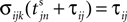 the spike is received by the postsynaptic neuron i, where it induces a phase jump according to Eq. 3. After spike reception we cancel the spike arrived (which has index k = 1) and renumber the indices k > 1 as k → k − 1 such that
  specifies the spike sent by neuron j which arrives next at the postsynaptic neuron i (cf. Figures 3
A,B for illustration).
specifies the spike sent by neuron j which arrives next at the postsynaptic neuron i (cf. Figures 3
A,B for illustration).
for some n, σijk(t) is set to The spike index k equals the number of spikes already in transit plus one. It thus depends on the actual network state at time Between two events σijk(t) increases linearly with slope one, when the spike is received by the postsynaptic neuron i, where it induces a phase jump according to Eq. 3. After spike reception we cancel the spike arrived (which has index k = 1) and renumber the indices k > 1 as k → k − 1 such that specifies the spike sent by neuron j which arrives next at the postsynaptic neuron i (cf. Figures 3
A,B for illustration).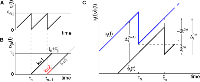
Figure 3. Phase dynamics of neuron j and definition of state variables. (A) At t = tn and t = tn + 1 the phase ϕj(t) reaches the threshold and is reset to 0. (B) The spikes emitted travel to the postsynaptic neurons i ∈ Post(j). They are described by σijk(t). In this example we show two spikes traveling from neuron j to one specific postsynaptic neuron i, described by σij1(t) (black) and σij2(t) (red). At t = tn, σij1(tn) is set to 0; here k = 1 because there is no spike in transit at  When neuron j spikes again at t = tn + 1, σij2(tn + 1) is set to 0. At t = tn + τij the spike emitted at t = tn arrives at the postsynaptic neuron i and induces a phase jump in ϕi(t) (not shown, cf. Figure 2
). After spike reception, we renumber k → k − 1 such that σij2 → σij1. (C) Definition of the phase shifts. The phase curve ϕi(t) of neuron i (blue) before and after the reception of a spike at t = tn is shown together with
When neuron j spikes again at t = tn + 1, σij2(tn + 1) is set to 0. At t = tn + τij the spike emitted at t = tn arrives at the postsynaptic neuron i and induces a phase jump in ϕi(t) (not shown, cf. Figure 2
). After spike reception, we renumber k → k − 1 such that σij2 → σij1. (C) Definition of the phase shifts. The phase curve ϕi(t) of neuron i (blue) before and after the reception of a spike at t = tn is shown together with  (black).
 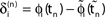 is the difference of neuron i’s phases in the unperturbed and the perturbed dynamics taken at corresponding event times tn and
  .
.  denotes the difference of event times tn and
  i.e. the temporal offset between both sequences. Finally,
  is some phase shift of neuron i with the temporal offset taken into account.
When neuron j spikes again at t = tn + 1, σij2(tn + 1) is set to 0. At t = tn + τij the spike emitted at t = tn arrives at the postsynaptic neuron i and induces a phase jump in ϕi(t) (not shown, cf. Figure 2
). After spike reception, we renumber k → k − 1 such that σij2 → σij1. (C) Definition of the phase shifts. The phase curve ϕi(t) of neuron i (blue) before and after the reception of a spike at t = tn is shown together with (black). is the difference of neuron i’s phases in the unperturbed and the perturbed dynamics taken at corresponding event times tn and . denotes the difference of event times tn and i.e. the temporal offset between both sequences. Finally, is some phase shift of neuron i with the temporal offset taken into account.Lyapunov Stability of Arbitrary Generic Spike Sequences
In this section we study the stability properties of the spike sequences. We compare the microscopic dynamics of two sequences, that slightly differ in the timing of the spikes, but have the same ordering. We show that the distance between these trajectories is bounded by the initial distance. Assuming that one sequence is generated by a perturbation of the other, this implies Lyapunov stability for the considered spike pattern. Distances and perturbation sizes are measured using the maximum norm.
Since the distance between trajectories only changes at event times, we can choose an event-based perspective. The time of the nth event in the entire network is denoted by tn in the first sequence, and by  in the second one. Analogously, we denote the phases of a neuron i at a given time t by ϕi(t) and
  and the spikes in transit at time t by σijk(t) and
  in the different sequences. Let
in the second one. Analogously, we denote the phases of a neuron i at a given time t by ϕi(t) and and the spikes in transit at time t by σijk(t) and in the different sequences. Let
denote the difference between the phase difference, 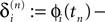
 and the temporal offset,
  after the nth and before the (n + 1)th event (cf. Figure 3
C). Similarly
after the nth and before the (n + 1)th event (cf. Figure 3
C). Similarly
and the temporal offset, after the nth and before the (n + 1)th event (cf. Figure 3
C). Similarly
labels the shift of the kth spike sent by neuron j and not yet arrived at neuron i after the nth and before the (n + 1)th event. Between two consecutive events, both  and
and  increase linearly and only at event times the phases and spike variables are updated nonlinearly as described above. Therefore, to study the stability of the system it is sufficient to consider the phase shifts after events.
and increase linearly and only at event times the phases and spike variables are updated nonlinearly as described above. Therefore, to study the stability of the system it is sufficient to consider the phase shifts after events.In the following we investigate the evolution of shifts at the discrete event times. There are two different kinds of events: (i) sending and (ii) receiving of spikes. In the first case, the shifts  and
and  stay unchanged, but new spikes with new spike variables are generated. These variables inherit the perturbation of the sending neuron. In the second case, the phase shift of the neuron which receives the spike changes and the spikes in transit are reordered. The resulting phase shift of the neuron receiving a spike turns out to be a weighted sum of previous shifts. This can be shown by studying both cases in detail.
and stay unchanged, but new spikes with new spike variables are generated. These variables inherit the perturbation of the sending neuron. In the second case, the phase shift of the neuron which receives the spike changes and the spikes in transit are reordered. The resulting phase shift of the neuron receiving a spike turns out to be a weighted sum of previous shifts. This can be shown by studying both cases in detail.Transfer of perturbations without change of size
If as (n + 1)th event the phase of some neuron j* reaches its threshold and a spike is emitted, the shifts of all neurons’ phases stay unchanged,

Similarly, the shifts of the spikes in transit stay unchanged
Additionally, new spikes are generated σij*k*(tn + 1) = 0 and  where k* = k*(i, j*, n + 1) is the appropriate spike number, cf. Figure 3
. The shifts of the new spike variables depend on the phase shift of the sending neuron j* according to
where k* = k*(i, j*, n + 1) is the appropriate spike number, cf. Figure 3
. The shifts of the new spike variables depend on the phase shift of the sending neuron j* according to
where k* = k*(i, j*, n + 1) is the appropriate spike number, cf. Figure 3
. The shifts of the new spike variables depend on the phase shift of the sending neuron j* according to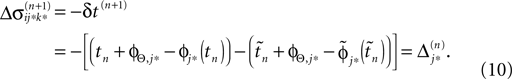
Averaging of prior perturbations
If as (n + 1)th event some spike arrives, say σi*j*1 (tn + 1) = τi*j*, it induces a phase jump in the postsynaptic neuron i*. According to Eq. 3, the phase shift  can be computed as:
can be computed as:
where  and
and  are the phases “just before” spike reception. Using the definitions (6) we find the identity
and are the phases “just before” spike reception. Using the definitions (6) we find the identity
Applying the mean value theorem in Eq. 11 and the relation
yields

where  is given by the derivative
is given by the derivative
for  for
for 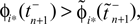 ϕ takes values ϕ ∈
  If neuron i* is not connected to neuron j*, εi*j* = 0, the function
  becomes the identity, such that the phase shift stays unchanged,
  indeed
  independent of ϕ.
for ϕ takes values ϕ ∈ If neuron i* is not connected to neuron j*, εi*j* = 0, the function becomes the identity, such that the phase shift stays unchanged, indeed independent of ϕ.For εi*j* < 0,  is bounded by
is bounded by
where  and
and  We have used that
  is monotonic increasing with ε
and We have used that is monotonic increasing with ε
The shifts of traveling spikes stay unchanged on spike reception, cf. Eq. 9,

for all spikes with i ≠ i* ∨ j ≠ j*. For i = i*, j = j* the spike variables are renumbered and

holds, except for k = 1, because σi*j*1 (t) is the variable describing the spike received and therefore canceled.
We will now ascertain that the coefficients  in Eq. 14 lie in a compact interval within (0, 1), such that a true averaging takes places when interactions happen. Formally, the phases of neurons can achieve values ϕi ∈ (−∞, ϕΘ,i]. Each neuron fires at least once within a time interval of length T, therefore the phases are certainly bounded to the compact interval ϕi ∈ [−T + ϕΘ,i, ϕΘ,i]. Further, in inhibitory networks the phase after an interaction is smaller than before,
in Eq. 14 lie in a compact interval within (0, 1), such that a true averaging takes places when interactions happen. Formally, the phases of neurons can achieve values ϕi ∈ (−∞, ϕΘ,i]. Each neuron fires at least once within a time interval of length T, therefore the phases are certainly bounded to the compact interval ϕi ∈ [−T + ϕΘ,i, ϕΘ,i]. Further, in inhibitory networks the phase after an interaction is smaller than before,
because together with Ui also  is strictly monotonic increasing and ε < 0. The strict concavity of Ui(ϕ) implies
is strictly monotonic increasing and ε < 0. The strict concavity of Ui(ϕ) implies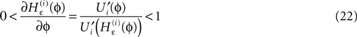
for any finite ϕ (cf. Figure 4
for illustration). The derivative  is continuous in ϕ, therefore the image of [−T + ϕΘ,i,ϕΘ,i] under the map
  is compact. Together with Eq. 22 it follows that
is continuous in ϕ, therefore the image of [−T + ϕΘ,i,ϕΘ,i] under the map is compact. Together with Eq. 22 it follows that
Figure 4. (A) The transfer function  for a leaky integrate-and-fire neuron. For ε = 0 (black),
  is the identity (black), for ε < 0 (blue: ε = −0.5, green: ε = −1) the phase ϕ after receiving an input is smaller than before. For all inhibitory inputs we find
  (B) The derivative of Ui(ϕ) is monotonic decreasing, therefore
  for ε ≤ 0 (cf. Eq. 22).
for a leaky integrate-and-fire neuron. For ε = 0 (black), is the identity (black), for ε < 0 (blue: ε = −0.5, green: ε = −1) the phase ϕ after receiving an input is smaller than before. For all inhibitory inputs we find (B) The derivative of Ui(ϕ) is monotonic decreasing, therefore for ε ≤ 0 (cf. Eq. 22).Taken together, Eqs. 8–10, 14 and 23 imply that a true averaging between shifts already present in the system takes place when a spike is received. For other events the shifts stay unchanged. As a consequence, the maximal and minimal shift after the nth event,

are bounded by the initial shifts for all future events,

as long as the order of events in both sequences is the same. Here the minima and maxima are taken over i,j ∈ {1,…,N} and k numbers the spikes traveling from neuron j to i at time tn. An initial perturbation cannot grow, thus the trajectory is Lyapunov stable. We note that we did not make any assumptions about the network connectivity, the results hold for any network structure and the described class of trajectories.
Asymptotic Stability
In this section we prove that for strongly connected networks even asymptotic stability holds under the condition that the perturbed and the unperturbed sequences have the same order of events, i.e. the order of events is unchanged by small perturbations. The central idea is as follows: We study the dynamics and convergence of two neighboring trajectories. We will track the propagation of the perturbation of one specific neuron l0 through the entire network. Since there is a directed connection between every pair of neurons in the network and any spike reception leads to an averaging of shifts, there is an averaging over all perturbations in the network. For large times all perturbations converge towards the same value, such that both sequences become equivalent, only shifted by a constant temporal offset. Further details and the derivation of the following Eqs. 26–28 is provided in the Appendix.
We find the upper bound

for the maximal perturbation after K := 2NM events and analogously the lower bound

for the minimal perturbation. The averaging factor c* is determined by the network parameters and bounded to

A bound for the difference of the maximal and minimal perturbation after K events is therefore given by

The spread of any perturbation through the network has a contracting effect on the total perturbation, it leads to a decay of the difference between the extremal perturbations at least by a factor (1 − c*). Inequality (29) implies together with the bound (28) that for the considered trajectories in the long-time limit the maximal and minimal perturbation are the same,

Thus, for t → ∞ the events are just shifted by a constant temporal offset

(cf. Figure 5
for illustration), and both sequences become equivalent 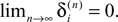 Thus all sequences considered are asymptotically stable for all strongly connected networks and perturbations decay exponentially fast with at least
Thus all sequences considered are asymptotically stable for all strongly connected networks and perturbations decay exponentially fast with at least
where ⌊·⌋ is the floor function. The actual and numerically measured exponential decay is much faster than the estimation given by Eq. 32, because for deriving Eqs. 26 and 27 in the Appendix we assumed a worst-case scenario. The main reasons for the faster decay are that (i) the mean path length is more meaningful for estimating the number of events until all neurons have received an input from the starting one and (ii) it is impossible that the neurons receive the worst-case perturbation at each reception.
Figure 5. Stable dynamics in the network of Figures 1
A–C. (A) Exponential decay of the maximal perturbation  (blue dots) and minimal margin κ(n) (gray line) for one microscopic dynamics. The initial perturbation
  decays exponentially fast. (B) Exponential convergence of the temporal offset δt(n). For large n the original and the perturbed sequences are equivalent, just shifted by a constant offset
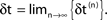
(blue dots) and minimal margin κ(n) (gray line) for one microscopic dynamics. The initial perturbation decays exponentially fast. (B) Exponential convergence of the temporal offset δt(n). For large n the original and the perturbed sequences are equivalent, just shifted by a constant offset Margins
The stability results in the previous sections hold for the class of patterns, where a small perturbation does not change the order of spikes. In this section we show that typical spike patterns, generated by networks with a complex connectivity, belong to this class.
In heterogeneous networks with purely inhibitory interactions the occurrence of events at identical times has a zero probability. There is no mechanism causing simultaneous spiking, like supra-threshold inputs in excitatorily coupled networks. As long as two events do not occur at the same event time, there is a non-zero perturbation size keeping the order unchanged in any finite time interval. However, the requirement of an unchanged event order yields more and more conditions over time such that the allowed size of a perturbation could decay more quickly with time than the actual perturbation. This is excluded if a temporal margin μ(n) (cf. Jin, 2002
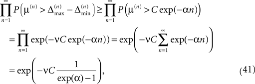
) stays larger than the dynamical perturbation for infinite time. Formally, after time tn denote the kth potential future event time (of the original trajectory) that would arise if there were no future interactions by θn,k, k ∈ ℕ, and the temporal margin by μ(n) := θn,2 − θn,1. A sufficiently small perturbation, satisfying 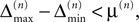 cannot change the order of the (n + 1)th event.
cannot change the order of the (n + 1)th event.Stability of generic periodic orbits
This directly implies that almost all periodic orbits (all those with non-degenerate event times tn) consisting of a finite number of P events are stable because there is a minimal margin

for every non-degenerate periodic pattern (c.f. also Memmesheimer and Timme, 2009 under revision).
Stability of irregular non-periodic spiking activity
We study the stability properties of irregular non-periodic spike sequences by considering the minimal margin κ(n) over the first n events. For simplicity, we consider delay distributions where τij is independent of the spike receiving neuron i. The irregular spiking dynamics of the entire network is well modeled by a Poisson point process with rate νs, where νs specifies the mean firing rate of the network (Tuckwell, 1988
; Brunel and Hakim, 1999
; Brunel, 2000
; Burkitt, 2006
). We assume that, along with the irregular dynamics, the temporal margins are also generated by a Poisson point process with the network event rate ν = 2νs, because any spike sending time generates one receiving event due to the independence of τij from i and the definition of events. The distribution function of margins is given by

Therefore, the probability that the minimal margin κ(n) after n events is smaller or equal to μ is determined by the probabilities that not all individual margins μ(n) are larger than μ such that

with density ρn(μ) := dP(κ(n) ≤ μ)/dμ = nνexp(−nνμ). This implies an algebraic decay with the number n of events for the expected minimal margin

that depends only on the event rate and is independent of the specific network parameters. Numerical simulations show excellent agreement with this algebraic decay (36); a typical example is shown in Figure 6
.
Figure 6. Margins in the network given in Figures 1
A–C. (A,B) Probability distribution P (κ(n) ≤ μ) after (A) n = 1 and (B) n = 105 events. The blue curve shows the distribution measured over 2500 samples, the red dotted line is the analytical prediction (no free fit parameter, rate ν is measured; cf. Eq. 35). (C) Algebraic decay of the average minimal margin,  (green dashed line, averaged over 250 random initial conditions) and its analytical prediction (no free fit parameter; black solid line). Additionally we show the minimal margin κ(n) for three exemplary initial conditions (gray lines), including that of Figure 5
A.
(green dashed line, averaged over 250 random initial conditions) and its analytical prediction (no free fit parameter; black solid line). Additionally we show the minimal margin κ(n) for three exemplary initial conditions (gray lines), including that of Figure 5
A.
(green dashed line, averaged over 250 random initial conditions) and its analytical prediction (no free fit parameter; black solid line). Additionally we show the minimal margin κ(n) for three exemplary initial conditions (gray lines), including that of Figure 5
A.This already strongly suggests that a sufficiently small perturbation stays smaller than the minimal margin for all times. However, in each step, the exponential distribution of margins has a finite density for arbitrary small values of μ, i.e. in each step the margin can fall below the level of perturbation with positive probability. We will show that  the probability that there is at least one step in which the margin falls below the perturbation size, goes to zero if the size of the initial perturbation goes to zero. Thus, also the probability that there is a change in the order of events goes to zero. Of course, we cannot expect to reach zero for nonzero perturbation.
the probability that there is at least one step in which the margin falls below the perturbation size, goes to zero if the size of the initial perturbation goes to zero. Thus, also the probability that there is a change in the order of events goes to zero. Of course, we cannot expect to reach zero for nonzero perturbation.We derive a lower bound for the probability that the margin stays larger than  for infinite time. We show that it converges to one when the size of the perturbation goes to zero and thus prove that sufficiently small perturbations have arbitrarily high probability to stay smaller than the minimal margin for all times. We start from the upper bound for the evolution of the perturbation, Eq. 32. Using
  and Eq. 28 leads to
for infinite time. We show that it converges to one when the size of the perturbation goes to zero and thus prove that sufficiently small perturbations have arbitrarily high probability to stay smaller than the minimal margin for all times. We start from the upper bound for the evolution of the perturbation, Eq. 32. Using and Eq. 28 leads to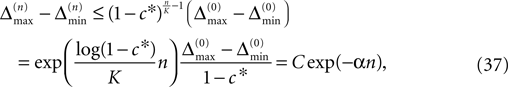
where we introduced
In particular, C → 0 if the initial perturbation goes to zero, i.e.  while α is independent of the initial perturbation. The probability that all margins are larger than all perturbations is given by
while α is independent of the initial perturbation. The probability that all margins are larger than all perturbations is given by
since the margins are independent. Using Eq. 37 and P(μ(n) > μ) = exp(−νμ) yields
which goes to one if the initial perturbation (and thus C) goes to zero.
We note that the assumption of a constant lower bound of the minimal margin is not necessary in contrast to Jin (2002)
. Indeed this assumption would be highly problematic, because in an irregular dynamics arbitrarily small margins naturally occur with positive probability in every step. So, assuming some lower bound would exclude generic irregular dynamics. In contrast, the novel approach introduced above enabled us to show that the generic irregular dynamics is stable.
For infinitely large networks in a mean field approach, where one takes the limit of infinitely many neurons in the beginning (e.g. v.Vreeswijk and Sompolinsky, 1996
, 1998
; Brunel and Hakim, 1999
), our method is not applicable in a straightforward way. In this limit the average inter-spike interval goes to zero and a positive margin cannot be presumed. In our analysis we employ the fact that the minimal margin stays finite, i.e. a sufficiently small perturbation does not change the order of events. This assumption and therefore our results hold for arbitrarily large finite systems.
Convergence to Periodic Orbits
Interestingly, the asymptotic stability together with the finite phase space imply that generic spike sequences converge to a periodic orbit. To show convergence analytically, we extend and explicate the ideas presented by Jin (2002) and Jahnke et al. (2008a)
. In the following we focus on a finite subsequence s* of a spike sequence generated by a given network. The number E* of events in s* is called the length E* of s*. As discussed towards the end of Section “Network Model”, the considered system is finite dimensional with dimension bounded from above by N + ND′. Thus, if s* is sufficiently long it contains at least two disjoint subsequences s1 and s2 of length E, where the ordering of events is identical. The maximal E for which the existence of s1 and s2 is guaranteed, is given by the largest integer E satisfying

When increasing the observation length E* also the possible length E of the subsequences increases. Both the phases and the variables encoding the spikes in transit are bounded to a finite interval, ϕi(t) ∈ [−T + ϕΘ,i,ϕΘ,i] and σijk(t) ∈ [0, maxij{τij}] at any given time t. Therefore, the maximal event-based distance between two trajectories is also bounded to a finite size,

Thus, comparing sequences s1 and s2 the initial event-based distance between their underlying trajectories at the beginning of s1 and at the beginning of s2 is bounded by Φmax, i.e.  By definition, the order of events in both sequences s1 and s2 is the same; therefore the distance between them shrinks according to Eq. 32. After E events the distance is bounded by (cf. Eq. 37)
By definition, the order of events in both sequences s1 and s2 is the same; therefore the distance between them shrinks according to Eq. 32. After E events the distance is bounded by (cf. Eq. 37)
where we used the definition (39). We note that, if we increase our observation length E* and therefore the subsequence length E, the maximal possible distance  between the trajectories underlying the sequences s1 and s2 decreases. If
  is sufficiently small, i.e. the distance between s1 and s2 after E events is smaller than the average margin, there is a high probability that also the order of events in the sequence following s1 and s2 are the same. Analogous to Eq. 41 the probability is given by:
between the trajectories underlying the sequences s1 and s2 decreases. If is sufficiently small, i.e. the distance between s1 and s2 after E events is smaller than the average margin, there is a high probability that also the order of events in the sequence following s1 and s2 are the same. Analogous to Eq. 41 the probability is given by: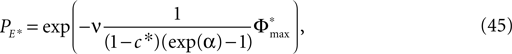
which goes to one when the observation length E* tends to infinity.
This implies a periodic dynamics: Assume that s1 occurs first in s* at the ath event and after a certain event number a + L ≤ E* − E the sequence s2 begins. We have seen that (with a certain probability) the ordering of events for (infinite) sequences starting at the ath and the (a + L)th event is the same for all future times. Therefore also the sequence starting at the (a + 2L)th event is identical to the ones mentioned before, so the ordering of events is periodic. Together with the exponential convergence of equally ordered sequences this implies that also the spike timings converge towards a periodic orbit. For arbitrarily long observed sequences this happens with an arbitrary large probability that tends to one as E* → ∞.
In Figure 7
we show a typical example: The mean margin,  decays algebraically on the transient and saturates after the periodic orbit is reached. Interestingly, the periodic attractor (shown in Figure 7
D) of the sparse random network resembles the “splay state” known from globally coupled networks (Strogatz and Mirollo, 1993
). In a splay state the firing pattern is characterized by equally spaced ISIs. It has been shown that it is possible to design networks, which exhibit more complex periodic spike patterns (Memmesheimer and Timme, 2006a
,b
). Indeed, in different parameter regimes we observe such complex periodic orbits, with a large periodicity, cf. the heterogeneous globally coupled network in Figure 8
, where the periodic orbit is reached after a small number of events compared to sparse networks. As shown previously (Timme et al., 2002
; Timme and Wolf, 2008
), highly irregular spiking activity may coexist with even the simplest (fully synchronous) periodic orbits that exhibits regular, maximally ordered activity.
decays algebraically on the transient and saturates after the periodic orbit is reached. Interestingly, the periodic attractor (shown in Figure 7
D) of the sparse random network resembles the “splay state” known from globally coupled networks (Strogatz and Mirollo, 1993
). In a splay state the firing pattern is characterized by equally spaced ISIs. It has been shown that it is possible to design networks, which exhibit more complex periodic spike patterns (Memmesheimer and Timme, 2006a
,b
). Indeed, in different parameter regimes we observe such complex periodic orbits, with a large periodicity, cf. the heterogeneous globally coupled network in Figure 8
, where the periodic orbit is reached after a small number of events compared to sparse networks. As shown previously (Timme et al., 2002
; Timme and Wolf, 2008
), highly irregular spiking activity may coexist with even the simplest (fully synchronous) periodic orbits that exhibits regular, maximally ordered activity.
Figure 7. Convergence towards a periodic orbit in a random network. (N = 40, γi ≡ 1, Ii ≡ 3.0, VΘ,i ≡ 1.0,  |Pre(i)| ≡ 8,
  ) (A) Coupling matrix, each realized connection is indicated by a black square. (B) Average minimal margin
  (averaged over 250 random initial conditions, cf. Figure 6
C) decays as a power-law (region A) and saturates after about 107 events (region B) when the periodic orbit is reached. Inset: Margin μ(n) (black) and minimal margin κ(n) (gray) for a trajectory started from one specific initial condition. The margin μ(n) fluctuates strongly on the transient and is comparatively large after the sequence becomes periodic; thus the minimal margin κ(n) does not decrease further for future events n. (C,D): Snapshots of irregular spike sequences (C) after n ≈ 15.000 events on the transient and (D) after n ≈ 108 events on the periodic orbit.
(averaged over 250 random initial conditions, cf. Figure 6
C) decays as a power-law (region A) and saturates after about 107 events (region B) when the periodic orbit is reached. Inset: Margin μ(n) (black) and minimal margin κ(n) (gray) for a trajectory started from one specific initial condition. The margin μ(n) fluctuates strongly on the transient and is comparatively large after the sequence becomes periodic; thus the minimal margin κ(n) does not decrease further for future events n. (C,D): Snapshots of irregular spike sequences (C) after n ≈ 15.000 events on the transient and (D) after n ≈ 108 events on the periodic orbit.
|Pre(i)| ≡ 8, ) (A) Coupling matrix, each realized connection is indicated by a black square. (B) Average minimal margin (averaged over 250 random initial conditions, cf. Figure 6
C) decays as a power-law (region A) and saturates after about 107 events (region B) when the periodic orbit is reached. Inset: Margin μ(n) (black) and minimal margin κ(n) (gray) for a trajectory started from one specific initial condition. The margin μ(n) fluctuates strongly on the transient and is comparatively large after the sequence becomes periodic; thus the minimal margin κ(n) does not decrease further for future events n. (C,D): Snapshots of irregular spike sequences (C) after n ≈ 15.000 events on the transient and (D) after n ≈ 108 events on the periodic orbit.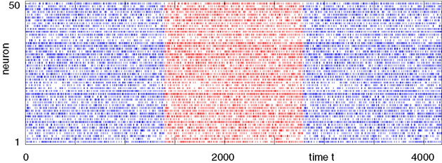
Figure 8. Long periodic orbit in a random network. (N = 50, γi ≡ 1, Ii ≡ 1.2, VΘ,i ≡ 1.0,  ) The coupling strengths are randomly independently drawn from the uniform distribution [−1, 0] and normalized afterwards
  The final spike pattern (shown after a transient of 9 × 10⁶ events) repeats every 11012 events and is highly irregular.
) The coupling strengths are randomly independently drawn from the uniform distribution [−1, 0] and normalized afterwards The final spike pattern (shown after a transient of 9 × 10⁶ events) repeats every 11012 events and is highly irregular.Although the attractor is reached after a finite number of events, the transient becomes very important in systems with strong inhibition or large number of neurons. As formerly found in networks with excitatory coupling (Zumdieck et al., 2004
), and also in weakly diluted networks with purely inhibitory interactions (Zillmer et al., 2006
), the transient length grows rapidly with network size such that the dynamics is governed by the transient for large time scales. We study inhibitory random networks with an arbitrary network structure, typically far away from the weakly diluted topology. To perform numerical measurements of the transient length in dependence on the network size N, we define the length of the transient, tr by the number of events after which the order of events stays periodic. When increasing the network size N, we leave the sum  of the external excitatiory current, Ii, and the internal inhibition,
  constant. Thus, on average each neuron receives a constant effective input independent of N and the mean firing rate of a single neuron 〈νi〉 is approximately conserved. Figure 9
shows the increase of transient lengths with network size for different sizes of internal inhibition and different scalings of the single connection strengths. We observe an exponential increase of the mean transient length with network size N independent of the scaling of the coupling strengths, εij, and the number of incoming connections, Ki := |Pre(i)|. This is qualitatively similar to the scaling of the transient lengths in weakly diluted networks (Zillmer et al., 2006
). Assuming that the rapid increase continues for much larger networks, the transient will dominate the dynamics essentially forever in networks of biological relevant sizes. In this sense the transient becomes quasi-stationary (cf. also Zillmer et al., 2006
, 2009
). If a larger network is in the balanced state (cf. Figure 1
), the stable transients typically dominate the network dynamics.
constant. Thus, on average each neuron receives a constant effective input independent of N and the mean firing rate of a single neuron 〈νi〉 is approximately conserved. Figure 9
shows the increase of transient lengths with network size for different sizes of internal inhibition and different scalings of the single connection strengths. We observe an exponential increase of the mean transient length with network size N independent of the scaling of the coupling strengths, εij, and the number of incoming connections, Ki := |Pre(i)|. This is qualitatively similar to the scaling of the transient lengths in weakly diluted networks (Zillmer et al., 2006
). Assuming that the rapid increase continues for much larger networks, the transient will dominate the dynamics essentially forever in networks of biological relevant sizes. In this sense the transient becomes quasi-stationary (cf. also Zillmer et al., 2006
, 2009
). If a larger network is in the balanced state (cf. Figure 1
), the stable transients typically dominate the network dynamics.
of the external excitatiory current, Ii, and the internal inhibition, constant. Thus, on average each neuron receives a constant effective input independent of N and the mean firing rate of a single neuron 〈νi〉 is approximately conserved. Figure 9
shows the increase of transient lengths with network size for different sizes of internal inhibition and different scalings of the single connection strengths. We observe an exponential increase of the mean transient length with network size N independent of the scaling of the coupling strengths, εij, and the number of incoming connections, Ki := |Pre(i)|. This is qualitatively similar to the scaling of the transient lengths in weakly diluted networks (Zillmer et al., 2006
). Assuming that the rapid increase continues for much larger networks, the transient will dominate the dynamics essentially forever in networks of biological relevant sizes. In this sense the transient becomes quasi-stationary (cf. also Zillmer et al., 2006
, 2009
). If a larger network is in the balanced state (cf. Figure 1
), the stable transients typically dominate the network dynamics.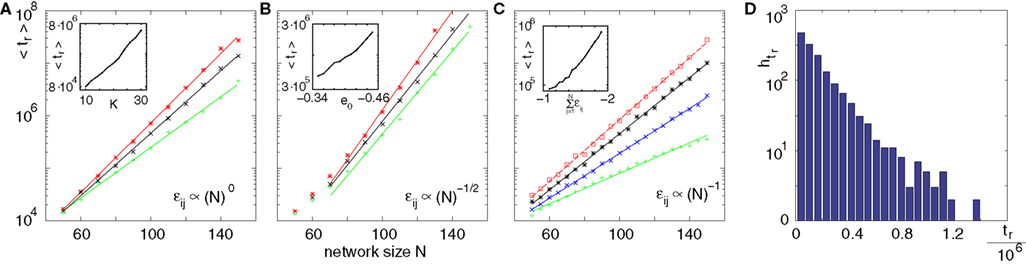
Figure 9. Scaling of the transient lengths in sparse random networks. (A) The sum of the external excitation and the internal inhibition is fixed,  such that the mean firing rate, 〈νi〉i, of the single neurons stays approximately constant. The number of incoming connections to each neuron, Ki := |Pre(i)|, is fixed to Ki ≡ 15 (green +), Ki ≡ 20 (black ×), Ki ≡ 25 (red *). The single connections are set to
  with e0 = −0.38. The solid lines show the best exponential fit. We observe an exponential increase of the trial averaged transient length 〈tr〉 with network size N. The inset shows the dependence of the transient length on the in-degree for fixed network size (N = 100). (B) Networks with fixed fraction of connections, where Ki ≡ ⌊pN⌋ and p = 1/4. We scale the coupling strengths as
  such that
  and the external current Ii is adjusted appropriately to fix the mean firing rate 〈νi〉i. The mean transient lengths for different e0 are shown together with the best exponential fit (e0 = −0.34 (green +), e0 = −0.38 (black ×), e0 = −0.42 (red *)). Again, we observe an exponential increase of the transient lengths with N. The inset shows the increase of the transient length with inhibitory coupling strength for fixed network size (N = 100). (C) Networks with fixed fraction of connections, where Ki ≡ ⌊pN⌋ and p = 1/4. The external currents Ii ≡ 3.0 are fixed and the internal coupling is normalized to
  (green +), −1.5 (blue ×), −1.75 (black *), −1.9 (red □), such that the mean firing rate, 〈νi〉i, of the single neurons is approximately the same for each curve. The number of incoming connections per neuron, Ki, increases linearly with network size, so the coupling strengths are scaled as εij ∝ 1/Ki. Here we also observe an exponential increase of 〈tr〉 with network size. The inset shows the fast increase of the transient length with inhibitory coupling strength for fixed network size and external current (N = 100, Ii ≡ 3.0). (D) The transient length is broadly distributed as shown in the histogram for 2500 trials started from random initial conditions, where the initial phases were randomly independently drawn from the uniform distribution on [0, 1] (N = 100, Ii ≡ 3.0,
  ).
).
such that the mean firing rate, 〈νi〉i, of the single neurons stays approximately constant. The number of incoming connections to each neuron, Ki := |Pre(i)|, is fixed to Ki ≡ 15 (green +), Ki ≡ 20 (black ×), Ki ≡ 25 (red *). The single connections are set to with e0 = −0.38. The solid lines show the best exponential fit. We observe an exponential increase of the trial averaged transient length 〈tr〉 with network size N. The inset shows the dependence of the transient length on the in-degree for fixed network size (N = 100). (B) Networks with fixed fraction of connections, where Ki ≡ ⌊pN⌋ and p = 1/4. We scale the coupling strengths as such that and the external current Ii is adjusted appropriately to fix the mean firing rate 〈νi〉i. The mean transient lengths for different e0 are shown together with the best exponential fit (e0 = −0.34 (green +), e0 = −0.38 (black ×), e0 = −0.42 (red *)). Again, we observe an exponential increase of the transient lengths with N. The inset shows the increase of the transient length with inhibitory coupling strength for fixed network size (N = 100). (C) Networks with fixed fraction of connections, where Ki ≡ ⌊pN⌋ and p = 1/4. The external currents Ii ≡ 3.0 are fixed and the internal coupling is normalized to (green +), −1.5 (blue ×), −1.75 (black *), −1.9 (red □), such that the mean firing rate, 〈νi〉i, of the single neurons is approximately the same for each curve. The number of incoming connections per neuron, Ki, increases linearly with network size, so the coupling strengths are scaled as εij ∝ 1/Ki. Here we also observe an exponential increase of 〈tr〉 with network size. The inset shows the fast increase of the transient length with inhibitory coupling strength for fixed network size and external current (N = 100, Ii ≡ 3.0). (D) The transient length is broadly distributed as shown in the histogram for 2500 trials started from random initial conditions, where the initial phases were randomly independently drawn from the uniform distribution on [0, 1] (N = 100, Ii ≡ 3.0, ).Robustness of Stability and Smooth Transition to Chaos
In the following we will check the robustness of our results. The considerations above hold for networks with inhibitory interactions without temporal extent. We investigate the influence of excitatory interaction and pulses with a finite duration. For small deviation from the networks considered above the stability properties are similar, for large fractions of excitatory connections and larger temporal extent we observe a transition to a chaotic regime. For temporally extended couplings we assume that after a neuron is reset all previous input is lost. Therefore the state of a neuron is specified by its last spike time and all spikes it has received afterwards. The phase representation is thus not meaningful anymore and we track two trajectories by comparing the differences in the last spiking times of the neurons and in the spike arrival times since these last spikings. To keep the section consistent, we adopt this view when studying the Lyapunov exponents of the excitatory dynamics.
Excitatory interactions
We have shown that in networks with purely inhibitory interactions the dynamics is typically stable. If the connection from neuron j to neuron i is excitatory, the phase shift  of the postsynaptic neuron i after receiving a spike from neuron j as the (n + 1)th event may exceed its shift
  before and the shift
  of the received spike. Figures 10
A,B gives an illustration: A spike is simultaneously received in the perturbed and in the unperturbed dynamics
of the received spike. Figures 10
A,B gives an illustration: A spike is simultaneously received in the perturbed and in the unperturbed dynamics  The phase shift before and after the application of the transfer function
  is shown for (A) an inhibitory input and (B) an excitatory input. For inhibitory input the phase shift
  is reduced, this leads to the stable dynamics as described in the sections above. For excitatory input, the phase shift
  increases when the spike is received.
of the postsynaptic neuron i after receiving a spike from neuron j as the (n + 1)th event may exceed its shift before and the shift of the received spike. Figures 10
A,B gives an illustration: A spike is simultaneously received in the perturbed and in the unperturbed dynamics The phase shift before and after the application of the transfer function is shown for (A) an inhibitory input and (B) an excitatory input. For inhibitory input the phase shift is reduced, this leads to the stable dynamics as described in the sections above. For excitatory input, the phase shift increases when the spike is received.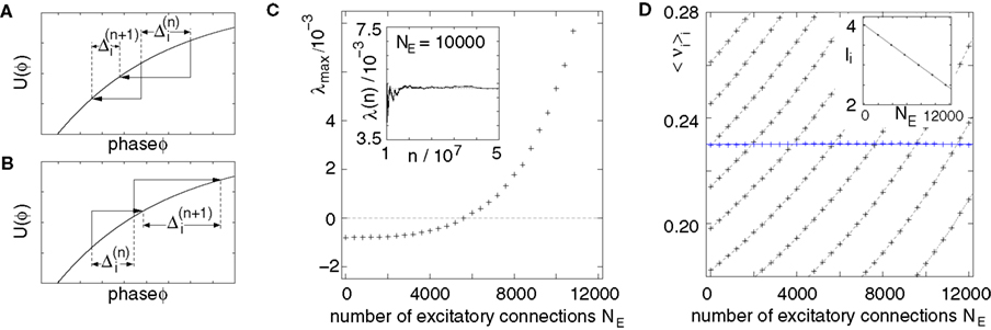
Figure 10. Destabilizing effect of excitation. (A) Simultaneous receiving of an inhibitory input decreases the phase shift. (B) Simultaneous receiving of an excitatory input increases the phase shift. (C) The largest Lyapunov exponent is measured for an increasing fraction of excitatory connections starting with the network of Figures 1
A–C and ending with the network of Figures 1
D–F. Here we keep the firing rate constant. Inset shows exemplarily the convergence of a finite time Lyapunov exponent with n. (D) Average firing rate 〈νi〉i versus number of excitatory connections in the network for different external currents Ii (black crosses, values belonging to the same Ii are connected by a dashed line). The neurons’ firing rate stays almost constant if we reduce the external current linearly with the number of excitatory connections (blue crosses). The inset displays the current strength employed to maintain firing rate of 〈νi〉i ≈ 0.23. (Further details see text).
Indeed, since the inverse of Ui(ϕ) is monotonically increasing with ϕ, we find for a given ε > 0

In contrast to Eq. 22, the derivative of the transfer function  is bounded from below by
is bounded from below by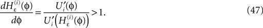
According to Eq. 14, this can lead to an increase of (in particular extremal) perturbations and to a destabilization of the trajectory. The upper bound of  cmax < 1 (cf. Eq. 23) does not hold anymore. However, in a network with a small fraction of excitatory connections, the trajectory is still stable. At an interaction the perturbation may increase, but the stabilizing effect of inhibitory inputs dominates the dynamics. We study the transition from the stable regime to chaotic dynamics (a discussion of the chaotic dynamics in networks with purely excitatory interactions can be found in Zumdieck et al., 2004
). When increasing the number of excitatory couplings, we increase the mean effective input current to the neurons. Thus we additionally decrease the external input Ii to keep the network rate ν constant. Indeed, in good approximation, the current has to be decreased linearly with NE, the number of excitatory connections, Ii ≡ I − kNE where i is the original input current.
cmax < 1 (cf. Eq. 23) does not hold anymore. However, in a network with a small fraction of excitatory connections, the trajectory is still stable. At an interaction the perturbation may increase, but the stabilizing effect of inhibitory inputs dominates the dynamics. We study the transition from the stable regime to chaotic dynamics (a discussion of the chaotic dynamics in networks with purely excitatory interactions can be found in Zumdieck et al., 2004
). When increasing the number of excitatory couplings, we increase the mean effective input current to the neurons. Thus we additionally decrease the external input Ii to keep the network rate ν constant. Indeed, in good approximation, the current has to be decreased linearly with NE, the number of excitatory connections, Ii ≡ I − kNE where i is the original input current.To quantify the transition we estimate the largest Lyapunov exponent of the system: At the nth event, we denote n − W(n) the earliest event which still influences the future dynamics of the system explicitly. We apply an initial perturbation of size ||Δ0||1 to the event times t0, t−1,…,t−W(0), where Δn = (Δtn, Δtn − 1,…,Δtn − W(n)) is the perturbation vector at the nth event time and Δti is the perturbation of ti. Here ||.||1 is the 1-norm, ||x||1 := Σi |xi|. We evolve the system and rescale the perturbation vector Δn by an after each event, such that the rescaled perturbation vector is of the same size as the initial perturbation,

The largest Lyapunov exponent, λmax, is then given by

We observe a transition from a stable to a chaotic regime, characterized by a positive Lyapunov exponent. For small fraction of excitatory neurons the dynamics is typically stable, the effect of the inhibitory pulses dominates the dynamics and, on average, a perturbation do not grow over time. With increasing NE the Lyapunov exponent increases until the dynamic becomes chaotic. Of course, in our simulations we can only study finite time Lyapunov exponents with very large n and estimate the value to which they converge. The chaotic dynamics may thus be transient. However, it dominates the dynamics at least over very long times.
Estimating the maximal Lyapunov exponent in networks including excitatory interactions can be difficult (Hansel et al., 1998
; Zumdieck et al., 2004
; Brette et al., 2007
; Cessac and Vieville, 2008
; Kirst and Timme, 2009
). Suprathreshold excitation, together with the infinitely fast response of neurons receiving a spike and the sharp threshold may induce synchronous events. Thus even an infinitesimal small perturbation may change the order of spikes. Nonetheless generically the perturbation will stay infinitesimal small, in particular for a small fraction of excitatory connections, such that we estimate the largest Lyapunov exponent in the following way: We evaluate at each time step the resulting temporal perturbation on the actual event as a result of earlier perturbation under the assumption that the order of spikes stays the same. This gives us the new perturbation vector Δn, which is rescaled according to (48). For long times, λ(n) then will give an estimate of the largest Lyapunov exponent and describe the generic behavior of the trajectory under the influence of sufficiently small perturbations. However, we cannot exclude the occurrence of macroscopic perturbations in general.
Figures 10
C,D show some numerical results: In Figure 10
C the largest Lyapunov exponent is measured for an increasing fraction of excitatory connections starting with the network of Figures 1
A–C and ending with the network of Figures 1
D–F. The number of excitatory connections is increased by successively choosing one incoming inhibitory connection per neuron to be excitatory. The external current, Ii, is reduced linearly to keep the network rate unchanged according to Ii ≡ I − kNE, where I = 4.0 is the initial external current, k ≈ 1.3 10−4 and NE is the number of excitatory connections. For a large fraction of excitatory couplings we observe a transition to an unstable, chaotic regime. The inset demonstrate the convergence of 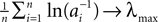 (exemplarily shown for NE = 10000). For a constant external current the rate increases with increasing fraction of excitatory connections (black crosses, for Ii ∈ {2.25, 2.5, 2.75, 3.0, 3.25, 3.5, 3.75, 4.0, 4.25, 4.5}). The neurons’ firing rate stays almost constant, if we reduce the external current linearly with the number of excitatory connections (blue crosses). We determined the value of Ii at the intersection point of the 〈νi〉i vs. NE curves with the desired frequency by linear interpolation. The values (Ii, NE) that give rise to the desired frequency lie in good approximation on a straight line with slope −k ≈ −1.3 10−4 (cf. Inset to (D)).
(exemplarily shown for NE = 10000). For a constant external current the rate increases with increasing fraction of excitatory connections (black crosses, for Ii ∈ {2.25, 2.5, 2.75, 3.0, 3.25, 3.5, 3.75, 4.0, 4.25, 4.5}). The neurons’ firing rate stays almost constant, if we reduce the external current linearly with the number of excitatory connections (blue crosses). We determined the value of Ii at the intersection point of the 〈νi〉i vs. NE curves with the desired frequency by linear interpolation. The values (Ii, NE) that give rise to the desired frequency lie in good approximation on a straight line with slope −k ≈ −1.3 10−4 (cf. Inset to (D)).The result is particularly remarkable since in mean-field descriptions of balanced networks, as long as the mean input to each cell is the same, the regime where NE = 0 is comparable to the regime where NE > 0 with appropriately reduced external excitatory current Ii.
Temporally extended interactions
Up to now, we considered δ-coupling, where the response to an action potential is instantaneous. However, in biological neuronal systems the postsynaptic current has finite temporal extent. In the following, we investigate the influence of such temporally extended interactions. The analysis gets more complicated, because neurons are permanently influenced by incoming signals. As mentioned above, in our model we assume that the neuron looses the information about previously received spikes when it reaches the threshold and is reset.
We modify Eq. 1 by introducing a temporally extended interaction kernel g(t), such that the evolution of the membrane potential is given by

In the following analysis we consider single exponential couplings, g(t) = Θ (t)·βe−βt with time scales γ−1 > β−1 > 0, the time constant of the postsynaptic current is shorter than the membrane time constant. As an exemplary neuron model we study the leaky integrate-and-fire neuron, fi(Vi) = −γVi(t) + Ii, but the analysis can easily be extended to more complex neuron models and interaction kernels.
Numerical simulations show that the stability of the dynamics is robust against introduction of synaptic currents with small temporal extent, but on increase of temporal extension a transition to chaos occurs. In Figure 11
A, the largest Lyapunov exponent, λmax, in a random network is estimated in dependence of the decay time constant β−1 of the synaptic current. For small time constant β−1, the dynamics behaves similar to the dynamics with δ-pulse interactions, in particular it is stable, the largest Lyapunov exponent is negative. For increasing β−1 the temporal extension becomes more and more influential and there is a transition to an unstable, chaotic regime with positive largest Lyapunov exponent.
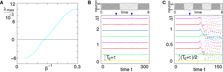
Figure 11. Robustness and transition to chaos with increasing temporal extent of the postsynaptic current. (A) Largest Lyapunov exponent λmax in a random network (N = 50, |Pre(i)| ≡ 10, γ = 1, Ii ≡ 4.0, 
 ) versus time constant β−1 of the synaptic current. (B) Stable periodic pattern in a network with temporally extended interactions. (C) Time compressed, thus unstable pattern in a network with temporally extended interactions. (For details see text).
) versus time constant β−1 of the synaptic current. (B) Stable periodic pattern in a network with temporally extended interactions. (C) Time compressed, thus unstable pattern in a network with temporally extended interactions. (For details see text).We now study the linear stability properties analytically. We denote the last spiking time of neuron i before tn by

at t = t0(n,i) the potential of neuron i was reset to zero. The solution of Eq. 50 together with the initial condition Vi(t0(n,i)) = 0 is then given between the nth and (n + 1)th network event by
where  is the reception time of the spike sent at
  by neuron j at neuron i. The sum in Eq. 52 takes into account all spikes which are received by neuron i between t0(n,i) ≤ t ≤ tn and therefore influence the potential Vi,n(t). In the limit of very short temporal extension of the postsynaptic current, β → ∞, Eq. 52 becomes a solution of Eq. 1. After the nth event, neuron i would reach the threshold at some time t′ under the assumption that there are no further inputs after tn. According to Eq. 52, t′ is implicitly given by
is the reception time of the spike sent at by neuron j at neuron i. The sum in Eq. 52 takes into account all spikes which are received by neuron i between t0(n,i) ≤ t ≤ tn and therefore influence the potential Vi,n(t). In the limit of very short temporal extension of the postsynaptic current, β → ∞, Eq. 52 becomes a solution of Eq. 1. After the nth event, neuron i would reach the threshold at some time t′ under the assumption that there are no further inputs after tn. According to Eq. 52, t′ is implicitly given by
where A is the vector of the original event times tn,…,tn − W,

where we introduced W = maxn{W(n)}. We now estimate the effect of a small perturbation Δtn,…,Δtn − W of the event times tn,…,tn − W on the hypothetical event time t′. By Eq. 53, the Jacobian of t′, Dt′, with respect to former spike times, tn,…,tn − W, is given as
The linearized estimation of the displacement Δt′of t′ is then given by
The special structure of Vi,n(t) (cf. Eq. 52), more precisely the fact that Vi,n(t) depends on t via t − tk for k ∈ {n − W,…,n}, yields the identity

Under the condition

we can combine Eqs. 56 and 57 and find bounds for the displacement

Condition (58) implies that if neuron i sends or receives a spike earlier, also the threshold is crossed earlier. This always holds for δ-couplings, for interactions with temporal extend it restricts the class of patterns as we show below. Equation 59 is an analog to Eq. 25, sufficiently small perturbations stay bounded by the initial ones for finite times. This directly implies Lyapunov stability for periodic orbits. For general irregular dynamics and to prove asymptotic stability, the propagation of pulses through the network has to be studied as for the nonlinear stability analysis in the main part.
We now want to specify a class of periodic patterns which are stable in a network with temporally extended synaptic currents. The influence of various events on Vi,n(A,t′) is as follows: For an influential spike receiving tk, Eq. 52 yields

where ε* < 0 is the coupling strength from the sending neuron. For the last spike sending of neuron i, tk = t0(n,i),

For any other event tk a displacement of tk has no influence on Vi,n(t), here
Therefore condition (58) reduces to a condition on the left and right hand side of Eq. 60 and can be reformulated as
where tk are the spikes arrival times at neuron i since the last reset t0(n,i). This means that the class of patterns where each neuron i does not cross the threshold for a time period Td after receiving a spike are stable. For β → ∞ the system tends to the δ – pulse coupled system and indeed Td vanishes,  such that any non-degenerated orbit is stable. However, for temporally extended interactions unstable periodic orbits exists and also chaotic dynamics is possible (cf. Figure 11
A).
such that any non-degenerated orbit is stable. However, for temporally extended interactions unstable periodic orbits exists and also chaotic dynamics is possible (cf. Figure 11
A).
such that any non-degenerated orbit is stable. However, for temporally extended interactions unstable periodic orbits exists and also chaotic dynamics is possible (cf. Figure 11
A).To illustrate our analytical findings, in Figures 11
B,C, we used a generalization of a recently introduced method (Memmesheimer and Timme, 2006a
,b
) to design two networks realizing predefined spike patterns in a network of five neurons (VΘ,i ≡ 1.0, Ii ≡ 2.4, β = 8, τ := τij ≡ 0.125) with temporally extended couplings. Both patterns are the same, but with different ISIs. In (B) all spikes are separated by ΔT = Td + τ, which ensures that a neuron never spikes within a time period Td after receiving a spike; in (C) we choose the ISIs smaller ΔT = (Td + τ)/2. The lower panels illustrates the stability properties: The spike times of the different neurons are plotted relative to the spike time of neuron 1 in vertical direction. The horizontal direction is simulated time, different colors indicate spike times of the five different neurons. At certain points in time (blue arrows) the network dynamics is perturbed. The dynamics in (B) is stable: After perturbations of size ≈0.2 (maximum norm), the dynamics converge towards the periodic orbit. (C) The dynamics is unstable: a perturbation of size ≈10−12 leads to a divergence from the unstable periodic orbit.
Irregular spiking activity that robustly arises in balanced state models constitutes a generic feature of cortical dynamics. Here, for a class of models including e.g. the common leaky integrate-and-fire neuron, we have shown that generic trajectories which give rise to the irregular balanced state can be exponentially stable. In particular, they are stable in purely inhibitory strongly connected networks of neurons with delayed couplings and with infinitesimal synaptic time course. We showed that the dynamics even converges to a periodic orbit. However, the length of the irregular yet stable transient grows rapidly with network size such that for larger networks, in particular for biological relevant sizes, transients may dominate the dynamics on all relevant time scales.
Furthermore, we found that the phenomenon of stable yet irregular dynamics is robust against introducing some excitatory interactions or against increasing the synaptic time scales from zero. If the synaptic responses become too slow or excitatory interactions too many, we revealed a smooth transition from stable irregular dynamics to chaotic, equally irregular dynamics. We emphasize that we kept the network rate during this transition (and thus keep the balance) and that the mean field descriptions (v.Vreeswijk and Sompolinsky, 1998
; Brunel, 2000
) of networks in both regimes are identical when the parameters are suitably chosen. Thus, highly irregular spiking dynamics occurs independent of the stability properties of the network.
Earlier studies on balanced neural activity considered a priori the limit of infinitely many neurons in sparse networks (v.Vreeswijk and Sompolinsky, 1996
, 1998
; Amit and Brunel, 1997
; Brunel and Hakim, 1999
; Brunel, 2000
). In this mean field limit the collective dynamics is well understood. In particular in infinitely large networks of binary neurons with balanced excitatory and inhibitory interactions the dynamics are chaotic (v.Vreeswijk and Sompolinsky, 1996
, 1998
). Further studies of finite networks found stable dynamics in weakly diluted networks of inhibitory coupled neurons (Zillmer et al., 2006
), as well as in globally coupled networks with dominating inhibition (Jin, 2002
). Recent analytical evidence confirmed the existence of stable dynamics in inhibitory coupled networks of integrate-and-fire neurons with a more complex structure (Jahnke et al., 2008a
). As the inter-event times that underly our analysis shrink inversely proportional to the network size (at a given individual neuron-spiking-rate), the methods applied here, however, are not applicable in a straightforward way in associated mean field models. Thus, one cannot make strict statements about stability in the limit of infinitely many neurons. Nevertheless, as shown above, generic transients and periodic trajectories in arbitrarily large inhibitorily coupled networks are stable.
Taken together, the results show that the microscopic dynamics in the considered purely inhibitorily coupled networks differs substantially from the dynamics of networks that explicitly include excitatory couplings. Whereas the latter may be chaotic, the former are generically stable – despite both showing the same irregularity features. In particular, chaotic as well as stable dynamics are equally well capable of generating highly irregular spiking activity. The smoothness of the transition to chaos, without essential change of the irregularity (e.g. of the large coefficients of variation) further suggests that chaos is not the main dynamical origin of the high irregularity. We thus suggest that a mechanism different from chaos contributes to the irregularity of cortical firing patterns in a substantial way.
Nevertheless, chaos as well as stochastic network properties such as unreliable synapses, may support the robust occurrence of irregular activity in cortical networks and also modify its computational features. It is thus an important future task to investigate which anatomical and dynamical features of cortical networks are indeed of crucial relevance for their spiking activity and their functions.
In the following we will derive the bounds Eqs. 26–28 stated in the Section “Asymptotic Stability”. We will track the propagation of the perturbation of one specific neuron l0 through the entire network.
All neurons spike at least once in a sufficiently large but finite time interval T. Moreover, after τmax = maxi,j(τij) all spikes in transit have certainly arrived at the postsynaptic neurons. We label the maximal number of events possible in the time interval [t,t + max{T,τmax}] by M. For purely inhibitory networks, M < ∞ due to the bounded neural spike rate. We denote the set of postsynaptic neurons of l0 by

thus a neuron li ∈ Posti(l0) is connected to l0 by a directed path of length i (cf. Figure 12
). Further, we define Post0(l0) := {l0}.
We estimate the bounds of the perturbation following one specific path from a neuron l0 to a neuron l. In a strongly connected network, l ∈ Postj(l0) for some j ≤ N − 1, so there is a directed path between l0 and l = lj via neurons l1,…,lj − 1 in the network. As the consideration holds for an arbitrary path, the result is an universal bound of the perturbation. Initially, at n = 0, the neurons are perturbed by  The first spiking of neuron l0 after n = 0 is labeled by s0 ≤ M. After a delay time
  this spike is received by the postsynaptic neuron l1 ∈ Post(l0), we call the event r1 ≤ 2M. After at most M further events, at s1 ≤ 3M, the neuron l1 emits a spike. In general, we recursively define si as the first spiking event of neuron li ∈ Posti(l0) after ri and ri as the event when the spike generated by li − 1 ∈ Posti − 1(l0) at si − 1 is received (cf. Figure 12
). Due to the definition of M, the relations si ≤ (2i+1)M and ri ≤ 2iM hold.
this spike is received by the postsynaptic neuron l1 ∈ Post(l0), we call the event r1 ≤ 2M. After at most M further events, at s1 ≤ 3M, the neuron l1 emits a spike. In general, we recursively define si as the first spiking event of neuron li ∈ Posti(l0) after ri and ri as the event when the spike generated by li − 1 ∈ Posti − 1(l0) at si − 1 is received (cf. Figure 12
). Due to the definition of M, the relations si ≤ (2i+1)M and ri ≤ 2iM hold.
The first spiking of neuron l0 after n = 0 is labeled by s0 ≤ M. After a delay time this spike is received by the postsynaptic neuron l1 ∈ Post(l0), we call the event r1 ≤ 2M. After at most M further events, at s1 ≤ 3M, the neuron l1 emits a spike. In general, we recursively define si as the first spiking event of neuron li ∈ Posti(l0) after ri and ri as the event when the spike generated by li − 1 ∈ Posti − 1(l0) at si − 1 is received (cf. Figure 12
). Due to the definition of M, the relations si ≤ (2i+1)M and ri ≤ 2iM hold.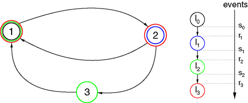
Figure 12. Tracking the propagation of a pulse. Here neuron l0 = 1 (black) is fixed as the initial neuron. The sets of postsynaptic neurons are: Post(1) = {2} (blue), Post2(1) = {1, 3} (green), Post3(1) = {1, 2} (red). Following one specific path through the network, we label the first spike event of neuron li ∈ Posti(l0) after receiving an input from li − 1 ∈ Posti − 1(l0) si. The event when the generated spike is received by li + 1 is labeled ri + 1. In a strongly connected network of size N the union  contains all the neurons, because any two of them are connected by a directed path of maximal length N − 1.
contains all the neurons, because any two of them are connected by a directed path of maximal length N − 1.First, we prove by induction that the perturbation of the neuron li, before sending of a spike at si, is bounded from above by

(1) Initially neuron l0 is perturbed by  Before l0 generates a spike it receives at most s0 − 1 inputs. According to Eq. 14, if the neuron l0 receives an input its perturbation may increase. To find an upper bound, we assume that at every event 0 < n < s0 neuron l0 receives an input with the maximal initial perturbation,
  and a minimal averaging constant cmin, which moves the average into the direction of the maximal possible perturbation. Repeated application of Eq. (14) yields
Before l0 generates a spike it receives at most s0 − 1 inputs. According to Eq. 14, if the neuron l0 receives an input its perturbation may increase. To find an upper bound, we assume that at every event 0 < n < s0 neuron l0 receives an input with the maximal initial perturbation, and a minimal averaging constant cmin, which moves the average into the direction of the maximal possible perturbation. Repeated application of Eq. (14) yields
which is the inductive statement (65) for i = 0.
(2) We assume that the statement (65) holds for  which is neuron li’s perturbation as inherited by the spike sent at si (cf. Eq. 10). After at most M events the spike is received by the postsynaptic neuron li + 1 at event ri + 1. In our worst- (or worse than worst-) case estimation, we assume that neuron li + 1 is maximally perturbed before it receives the spike,
  and that the interaction factor
  is maximal, cmax, such that again the average is moved into the direction of the maximal perturbation. Therefore the perturbation after the interaction is bounded by
which is neuron li’s perturbation as inherited by the spike sent at si (cf. Eq. 10). After at most M events the spike is received by the postsynaptic neuron li + 1 at event ri + 1. In our worst- (or worse than worst-) case estimation, we assume that neuron li + 1 is maximally perturbed before it receives the spike, and that the interaction factor is maximal, cmax, such that again the average is moved into the direction of the maximal perturbation. Therefore the perturbation after the interaction is bounded by
Before si + 1 > ri + 1 > si, neuron li + 1 receives at most (si + 1 − 1 − ri + 1) inputs. Analogously to Eq. 66, we assume that with each event li + 1 receives a spike which is maximally perturbed (with  ), and the averaging constant is minimal, cmin. This yields
), and the averaging constant is minimal, cmin. This yields
We replace  by
by  in Eq. 68, thereby increasing the right-hand side, because si − 1 − ri + 1 < 0. This directly yields the induction statement for
by in Eq. 68, thereby increasing the right-hand side, because si − 1 − ri + 1 < 0. This directly yields the induction statement for Based on Eq. 65, we now derive an upper bound of the perturbation of all neurons after event sN − 1. After this event, every neuron has sent at least one spike which is influenced by the initial perturbation of neuron l0, because in a strongly connected network the union  contains all neurons of the network (cf. Figure 12
). After the sith event, neuron li can still receive spikes. Before the sN − 1th event, taken as reference, it receives in the worst case scenario (sN − 1 − si) inputs with maximal initial perturbation
contains all neurons of the network (cf. Figure 12
). After the sith event, neuron li can still receive spikes. Before the sN − 1th event, taken as reference, it receives in the worst case scenario (sN − 1 − si) inputs with maximal initial perturbation  and minimal averaging factor cmin. Using Eq. 65 we repeatedly apply Eq. 14 (sN − 1 − si) times which leads to
contains all neurons of the network (cf. Figure 12
). After the sith event, neuron li can still receive spikes. Before the sN − 1th event, taken as reference, it receives in the worst case scenario (sN − 1 − si) inputs with maximal initial perturbation and minimal averaging factor cmin. Using Eq. 65 we repeatedly apply Eq. 14 (sN − 1 − si) times which leads to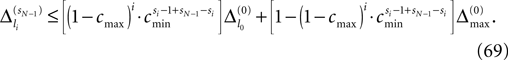
The right-hand side increases with i, therefore the perturbation of an arbitrary neuron j ∈ {1,…,N} after sN − 1 events is bounded from above by
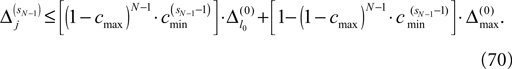
At the sN − 1th event there can be D′ spikes per neuron in transit which are, in the worst-case scenario, assumed to have the maximal perturbation. Due to their arrival after the sN − 1th event, the perturbations of neurons can still increase. However, after sN − 1 + M events all spikes generated before the sN − 1th event have arrived at the corresponding postsynaptic neurons. Taking into account the arrival of these spikes using Eqs. 14 and 70, we find an upper bound for the perturbation after sN − 1 + M events,
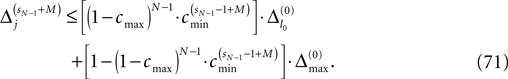
Due to the fact that generated spikes inherit a perturbation present in the phases at spike sending time, the bound (71) holds also for the perturbation of spikes generated after the sN − 1th and before the (sN − 1 + M)th event, because the bound (71) limits the maximal perturbation for all neurons between the sN − 1th and the (sN − 1 + M)th event.
We conclude that the perturbations of the neurons and the spikes in transit after K := 2NM ≥ sN − 1 + M events are bounded by
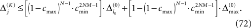
Therefore, we find an upper bound for the maximal perturbation  after K events,
after K events,
with
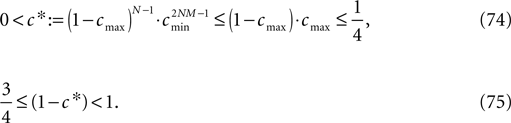
Similarly, we find a lower bound for the minimal perturbation after K events

by an estimation analogous to the one above, where only  has to be replaced
  and the relation “≤” has to be replaced by “≥”. We note, that we did not have to specify the perturbation
  to derive this result.
has to be replaced and the relation “≤” has to be replaced by “≥”. We note, that we did not have to specify the perturbation to derive this result.The authors declare that the research was conducted in the absence of any commercial or financial relationships that could be construed as a potential conflict of interest.
We thank Fred Wolf for helpful comments, David Hansel for pointing out the article (Zillmer et al., 2009
) and the Federal Ministry of Education and Research (BMBF) Germany for partial support under Grant No. 01GQ0430. RMM thanks the Sloan Swartz Foundation for partial support.
Brette, R., Rudolph, M., Carnevale, T., Hines, M., Beeman, D., Bower, J. M., Diesmann, M., Morrison, A., Goodman, P. H., Harris, F. C. Jr, Zirpe, M., Natschlager, T., Pecevski, D., Ermentrout, B., Djurfeldt, M., Lansner, A., Rochel, O., Vieville, T., Muller, E., Davison, A. P., El Boustani, S., and Destexhe, A. (2007). Simulation of networks of spiking neurons: a review of tools and strategies. J. Comput. Neurosci. 23, 349–398.