Department of Computer Science, University of Western Ontario, London, ON, Canada
Recent research has showed that tile systems are one of the most suitable theoretical frameworks for the spatial study and modeling of self-assembly processes, such as the formation of DNA and protein oligomeric structures. A Wang tile is a unit square, with glues on its edges, attaching to other tiles and forming larger and larger structures. Although quite intuitive, the idea of glues placed on the edges of a tile is not always natural for simulating the interactions occurring in some real systems. For example, when considering protein self-assembly, the shape of a protein is the main determinant of its functions and its interactions with other proteins. Our goal is to use geometric tiles, i.e., square tiles with geometrical protrusions on their edges, for simulating tiled paths (zippers) with complex neighborhoods, by ribbons of geometric tiles with simple, local neighborhoods. This paper is a step toward solving the general case of an arbitrary neighborhood, by proposing geometric tile designs that solve the case of a “tall” von Neumann neighborhood, the case of the f-shaped neighborhood, and the case of a 3 × 5 “filled” rectangular neighborhood. The techniques can be combined and generalized to solve the problem in the case of any neighborhood, centered at the tile of reference, and included in a 3 × (2k + 1) rectangle.
During the last decade, breakthroughs in DNA manipulation techniques have generated a wide range of advances in several areas of science: genetics, biology, medicine, but also nanoengineering and computer science. Regarding computer science in particular, several new directions of research have been established: DNA computing, DNA code-design, bioinformatics, computational modeling, and others. However, as usual in mathematics and computer science, the theoretical foundations of these new research topics lie deep in well established theoretical backgrounds.
The principle of self-assembly is one of the key concepts of nanosciences. It is the process by which objects aggregate independently, without external force or guidance, to form complex structures. This process can be found in nature at all levels: atoms interact with one another and create molecules, molecules may aggregate to form macromolecules, proteins self-assemble into protein complexes, etc. This natural principle has been mimicked successfully by artificial and semi-artificial self-assembly systems. Examples are the macroscopic plastic tiles of Rothemund (2000
) which assemble on an oil/water surface, simulating in this way a one-dimensional cellular automaton, or the self-assembly of some lead structures on a copper surface from Plass et al. (2001
). On the other hand, scientists have also used the intrinsic properties of biomolecules, such as the Watson–Crick complementarity of DNA molecules, in order to construct various self-assembly systems which are capable of a wide range of computations or tasks. Examples are the DNA nanostructures performing bit-wise cumulative XOR (Mao et al., 2000
), binary counters (Barish et al., 2005
), molecular switches between two conformations (Liedl et al., 2006
), DNA “walkers” moving along a track (Sherman and Seeman, 2004
), autonomous molecular motors (Bath et al., 2005
), nanoscale DNA shapes and patterns (Rothemund, 2006
), fixed-width cellular automata (Fujibayashi et al., 2008
), and many others.
Tile systems are one of the most important mathematical models of self-assembly systems (see e.g., Adleman, 2000
; Rothemund et al., 2004
). A Wang tile is an oriented unit square with each edge covered by a specific “glue”. Tiles are placed on the two-dimensional plane, and two adjacent tiles stick together if and only if they have the same glue on their abutting edges. Wang tiles, first proposed by Wang (1961
), have been extensively studied before finding their natural applications to self-assembly. More recently, Wang tiles and some of their variants, e.g., the Tile Assembly Model (Winfree, 1998
; Rothemund, 2001
), have been widely used as models for self-assembly and used to design and analyze successful practical experiments (see e.g., Rothemund et al., 2004
; Barish et al., 2005
).
Although quite intuitive, the idea of glues placed on the edges of a tile is not always natural for simulating the interactions occurring in some real systems. For example, when considering protein self-assembly, the shape of a protein is essential in determining its function and its interactions with other proteins. Tiles of various shapes had been previously designed and studied in the literature for specific purposes. For example, Robinson (1971)
designed six polygonal tiles (squares with notched edges and corners) in the context of solving the problem of minimization of the number of tiles that allowed only aperiodic tilings of the plane. In this paper, we design geometrical tiles, i.e., square tiles with protrusions on their edges, for the purpose of simplifying neighborhood relationships in tiling systems. Our main goal is to simulate any tiled path (“zipper”) that uses tiles with an arbitrarily complex neighborhood, by a “ribbon” of new geometrical tiles with a much simpler neighborhood relationship. Namely, the only requirement of a tiling with the new tiles is that no overlap occurs.
The reason we focus on tiled paths, either zippers or ribbons, instead of simple total or partial tilings, is threefold. First, from a theoretical point of view, due to their underlying path, the transition from zippers with complex neighborhoods to ribbons of geometrical tiles is much more complex than a simple transition between two, possibly partial, tilings (the first using a complex neighborhood and the second using geometric tiles). Indeed, preserving the underlying path of the zippers when transforming them into ribbons can be non-trivial. The second and third reasons are more application oriented. Note that the zipper and the ribbon structures are closely related to protein structures. Although we can see a protein as a “valid tiled” three-dimensional structure, these organic compounds are made of linear chains of amino acids, which are folded into their actual three-dimensional shape. The final reason for considering paths associated with tilings comes from the practical challenge of creating self-assembling nano-wires and nano-circuits. This aspect has been particularly studied in reference with the Tile Assembly Model (see e.g., deLorimier et al., 2002
; Cook et al., 2004
; Brun and Reishus, 2009
).
The first step towards solving the proposed problem was done in Czeizler and Kari (Submitted) where we introduced a “motif” construction, based on a geometrical tile design, that solved the problem in the case of Moore neighborhood. This paper is the next step towards the solution to the general case. We namely consider other natural extensions of the von Neumann and Moore neighborhoods, consisting of elements placed further away from the reference tile. In particular, we consider the case of the neighborhood that is a “tall” version of the von Neumann neighborhood (the neighborhood of a tile consists of the tile at the East, the tile at the West, two tiles to the North and two tiles to the South), the f-shaped neighborhood, and the 3 × 5 “filled” rectangular neighborhood. The techniques can be combined and generalized to solve the problem in the case of any neighborhood included in a Moore-type rectangular neighborhood, centered at the tile of reference, and of width 3 and height 2k + 1.
For all three cases, any zipper can be simulated by a ribbon made of new geometrical tiles in which the tiles shapes, and not their glues, determine the self-assembly process, and the neighborhood dependency is greatly simplified. The geometrical tile design ensures the transmission of information at a distance (across several tiles), as well as across several information channels. At the same time, the design satisfies the requirement of no overlapping between any two geometric tiles.
The paper is organized as follows. The next section presents basic definitions and notations. In Section “From Complex Neighborhoods to Geometric Tiles” we make the transition from tiles with complex neighborhoods to geometric tiles with simple, i.e., local, neighborhoods. The three following subsections address the case of the “tall” von Neumann neighborhood, the f-shaped neighborhood, and the 3 × 5 “filled” rectangular neighborhood. In the last section we show how to combine and generalize these techniques to solve the problem of neighborhood simplification by geometric tile design in the case of any neighborhood, centered at the tile of reference, and included in a 3 × (2k + 1) rectangle.
A Wang tile is an oriented unit square, i.e., a square which cannot be rotated or reflected, whose edges are labeled by symbols from a finite alphabet X, called glues. Thus, each tile t is uniquely determined by the four glues of its North, East, South and West edges as:
t=(tN, tE, tS, tW) ∈ X4.
The positions of the tiles on the plane are indexed by pairs of integers, (i, j) ∈ ℤ2.
A tile system T is a finite collection of tiles. We say that two tiles t and t′ stick on the North-South direction if and only if tN=t′S, that is, if the North end of t and the South edge of t′ have the same glue. Similarly, we can define the sticking property on the East-West, South-North and West-East directions.
A total tiling of the plane is a mapping 𝒯 : ℤ2 → T which assigns to every position from ℤ2 a tile from T. We say that a tiling 𝒯 is valid on a position (i, j) ∈ ℤ2 if the tile on position (i, j), denoted as t(i, j), sticks on the North-South, East-West, South-North and West-East directions to the tiles t(i, j + 1), t(i + 1, j), t(i, j − 1), and t(i − 1, j) respectively; here, we assume that there exists a tile on all positions of the plane.
A partial tiling of the plane is a mapping 𝒯D from a domain D ⊆ ℤ2 to T. We say that 𝒯D is valid if for any tile within the domain there are no mismatches between the glues of a tile and the glues of its existing neighbors. More formally, for all (i, j) ∈ D,
• if (i, j + 1) ∈ D then t(i, j)N=t(i, j + 1)S;
• if (i + 1, j) ∈ D then t(i, j)E=t(i + 1, j)W;
• if (i, j − 1) ∈ D then t(i, j)S=t(i, j − 1)N;
• if (i − 1, j) ∈ D then t(i, j)W=t(i − 1, j)E.
If no confusion can arise, we refer to valid tilings (either total or partial ones) simply as tilings.
A path P is a succession of adjacent positions in the plane. Formally, a finite (resp. infinite) path is a mapping P : I → ℤ2 where I={1, 2, 3,…,n}, n ≥ 2, (resp. I=ℕ) such that for all 1 ≤ i ≤ n − 1 (resp. for all i ≥ 1), if P(i)=(x, y) for some x, y ∈ ℤ, then P(i + 1) ∈ {(x, y + 1), (x + 1, y), (x, y − 1), (x − 1, y)}. A T-tiled path is a contiguous succession of tiles. Formally, it is a pair (P, r) where P : I → ℤ2 is a path and r : range(P) → T is a mapping assigning tiles to all positions of the path. A T-tiled path is called a T-ribbon if P is injective, i.e., the path is not self-crossing, and for any position in the path (except for the last one, if any), the tile and its successor must agree on their glues on the corresponding abutting edges. A T-zipper is a special type of T-ribbon where if two tiles are adjacent, even if they are not on consecutive positions on the path, they still must agree on their glues on their abutting edges. Given a ribbon (resp. a zipper) (P, r), we refer to P as the underlying path of the ribbon (resp. of the zipper).
A neighborhood vector (or simply neighborhood) is a finite collection of pairs of integers, describing the relative position in space of those tiles which interact with a given tile. Formally (Kari, 2005
; Adleman et al., 2009
), a neighborhood is an n-tuple N=(ν1, ν2,…,νN), νi ∈ ℤ2\{(0, 0)}, 1 ≤ i ≤ n, where νi ≠ νj for all 1 ≤ i < j ≤ n, and for all 1 ≤ i ≤ n there exists a unique j such that νi=(x, y) and νj=(−x, −y), where x, y ∈ ℤ. This last restriction on the content of the neighborhood vector is referred to as the “symmetry condition” and it is due to the fact that whenever a tile t interacts with another tile t′, then also t′ interacts with t. The neighbors of a position (x, y) ∈ ℤ2 are the positions (x + xi, y + yi) where νi=(xi, yi) for 1 ≤ i ≤ n.
In this paper, we consider the way in which a tile interacts with its neighbors to be similar to the case of classical Wang tiles, that is using glues. Although the tiles are represented as unit squares and placed on the nodes of a square lattice (exactly as in the case of classical tiles), we can think of a tile t as having n “virtual” edges, each labeled by a glue and each associated to exactly one neighboring tile. Given a neighborhood vector N=(ν1, ν2,…,νN) and a tile t placed on position (x, y) ∈ ℤ2, the neighboring tiles of t are all the tiles placed on the neighboring positions of (x, y), that is, the tiles on positions (x + xi, y + yi), where νi=(xi, yi) for all 1 ≤ i ≤ n. Then, each tile t is uniquely determined by an n-tuple of glues, t=(t1, t2,…,tn), where each glue ti ∈ X, 1 ≤ i ≤ n, corresponds to the virtual edge associated with the neighboring tile placed on the relative position νi.
In order to simplify future considerations, for a tile t, we use t(xi,yi) to refer to the glue ti, where νi=(xi, yi). Then, for two neighboring tiles t and t′ such that t′ is placed on the position νi relative to the position of t, the glues t(xi,yi) and  correspond to the common virtual edge between the two tiles. Note that the existence of the element (−xi, −yi) in the neighborhood N is guaranteed by the “symmetry condition”.
correspond to the common virtual edge between the two tiles. Note that the existence of the element (−xi, −yi) in the neighborhood N is guaranteed by the “symmetry condition”.Given a neighborhood vector N with n elements, a tile system using this neighborhood is a finite set TN ⊆ Xn of tiles. If no confusion can arise regarding the neighborhood, we can omit N from the notation. Then, a (partial) tiling is a (partial) function T : ℤ2 → T. If the function is defined for (x, y) ∈ ℤ2, we denote by t(x, y) the tile on this position.
Given a neighborhood vector N=(ν1, ν2,…,νN) and some D ⊆ ℤ2, we say that a (total or partial) tiling 𝒯 : D → T is valid on position (x, y) ∈ D if for all νi=(xi, yi) such that (x + xi, y + yi) ∈ D, we have t(x,y)(xi,yi) = t(x+xi,y+yi)(−xi,−yi), i.e., the two neighboring tiles have the same glue on their common virtual edge. We say that 𝒯 is valid if it is valid on all positions (x, y) ∈ D.
Next, we give a couple of examples illustrating the previous notions.
Example 1: let N be the well known von Neumann neighborhood vector,
N=((0, 1), (1, 0), (0, −1), (−1, 0)),
pointing to the positions to the North, East, South and West of a given tile. Tile systems using this neighborhood are exactly the classical Wang tile systems defined in Section “Preliminaries”. The neighbors of a given tile t(x, y) are those tiles placed to the North, East, South and West directions and the virtual edges of t(x, y) are simply its edges.
Example 2: let N be the “tall” von Neumann neighborhood vector, i.e.,
N=((0, 1), (0, 2), (1, 0), (0, −1), (0, −2), (−1, 0)).
In this case, the neighbors of a tile are the tiles placed one and two steps to the North and to the South, and the tiles placed immediately to the East and to the West. Here, besides the four normal edges of the tile, i.e., the four geometrical edges of the unit square, we have two additional virtual edges, one corresponding to the tile two steps to the North, and the other corresponding to the tile two steps to the South. In Figure 1
we present a valid partial tiling using this neighborhood. Note that adjacent tiles do not necessary have the same glues on their virtual edges; for instance, in Figure 1
, the North virtual edge of the tile t1 has to agree only with the South virtual edge of t2.
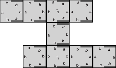
Figure 1. A partial tiling using the “tall” von Neumann neighborhood. The gray sections on the borders of the tiles represent the virtual edges.
Example 3: another well established instance is the Moore neighborhood vector,
N=((0, 1), (1, 1), (1, 0), (1, −1)(0, −1), (−1, −1), (−1, 0), (−1, 1)).
In this case, the neighbors of a given tile are all those tiles on the eight surrounding positions. Here, it is more intuitive to consider the corners of the tiles as the virtual edges, see Figure 2
for a valid partial tiling using this neighborhood.
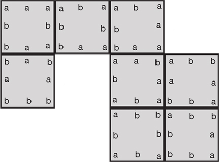
Figure 2. A partial tiling using the Moore neighborhood; both the edges and the corners of each tile are labeled by glues.
The notions of path, tiled path, and zipper are generalized in the natural way for the case of complex neighborhood vectors. The notion of path (resp. tiled path) remains unchanged independent of the contents of the neighborhood vector, i.e., a mapping P : I → ℤ2 (resp. a pair (P, r)) where the element P(i + 1) can be placed only to the North, East, South or West of P(i), exactly as in the case of classical Wang tile systems. In the case of zippers we require that the underlying path is not self-crossing and, moreover, any two tiles placed one on the neighborhood of the other (not necessarily succeeding or even adjacent to each other) must have the same glues of their common (maybe virtual) edges.
The principle of matching glues, although quite intuitive and very easy to be modeled mathematically, is not always natural for simulating the interactions within some self-assembly systems. Sometimes, the geometry of the objects involved in these systems can play the central role in their self-assembly. Thus, a major requirement for two or several objects to successfully aggregate is that when doing so, the objects will simply not overlap. For instance, in the case of protein self-assembly, the shape of the protein, i.e., its folding, determines both its function and the way it interacts with other proteins.
The most natural question arising at this moment is whether one can modify the structure of the tiles from the previous section such that instead of using glues as a way to control self-assembly, the shape of the tiles would govern the self-aggregation process. The case of finite zipper structures is particularly interesting, as this would correspond to a sequence of amino acids forming a protein, or a sequence of proteins forming a complex. The case of the classical von Neumann neighborhood has already been addressed by, e.g., Robinson (1971)
, Adleman et al. (2002
, 2009
), Kari (2003
), where glues were replaced with pairs of matching bumps and dents. However, in this case, each tile has abutting edges with all its neighbors, thus making the construction very intuitive. In the case of more complex neighborhood vectors, tiles may have virtual edges with some non-abutting neighbors. Thus, we must find a way to “transmit” information from one tile to its distant neighbors. In Czeizler and Kari (Submitted) we present a way of doing so for the case of tile systems using the Moore neighborhood vector from Example 3. However, also in this case, the neighbors of a tile are still surrounding it in some sense, making the construction easier.
When simulating a tiling using glues and a complex neighborhood dependency by a tiling based only on the non-overlapping principle, one of the first methods that one could try is the following. First, one simulates the first tiling by another one where tiles use the von Neumann neighborhood, i.e., using Wang tiles. Then, based on the already known constructions, one simulates the Wang tiling by another one where tiles use only their shapes in order to self-assemble.
One of the methods used in the literature (see e.g., Kari, 1989
; Adleman et al., 2002
, 2009
), for simulating a larger neighborhood by a smaller one, is to scale up the construction. That is, one creates some macro-tiles, which capture the information of both the initial tile and its neighbors. For instance, in Adleman et al. (2002
, 2009
), for the case of total tilings of the plane, the authors simulate the Moore neighborhood dependency by the von Neumann neighborhood dependency. The authors replace the initial tiles (let us call them mini-tiles) with a set of macro-tiles, consisting of blocks of 3 × 3 mini-tiles with no mismatching inside the blocks. Then, two such macro-tiles can be placed one North of the other if and only if the bottom 2 × 3 mini-tiles from the first macro-tile are exactly the same as the top 2 × 3 mini-tiles from the second macro-tile. Similarly, one defines the South-North, East-West and West-East sticking property. Then, by performing the following transformation, there exists a one-to-one correspondence between total tilings of the mini-tile system using the Moore neighborhood, and total tilings of the macro-tile system using the von Neumann neighborhood (Adleman et al., 2002
, 2009
). For a given total tiling using mini-tiles we replace each tile t(i, j) on position (i, j) with the macro-tile corresponding to the 3 × 3 block containing t(i, j) in the middle and all eight surrounding tiles. For the converse, the correspondence is obtained by associating to each macro-tile the mini-tile placed in the middle of that particular 3 × 3 block.
This technique can be generalized successfully for any neighborhood vector, by taking k × k blocks as macro-tiles, for sufficiently large k. However, it is essential to notice that this scaling up technique works only if we consider total tilings of the plane. If, on the other hand, we consider partial tilings, then this method generates errors, as we can design some valid partial tilings using macro-tiles which do not correspond to any valid tilings using mini-tiles, see, e.g., Figure 3
.
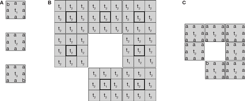
Figure 3. (A) A set of mini-tiles, (B) a valid tiling using macro-tiles, emphasizing the center mini-tiles, (C) the associated non-valid tiling using mini-tiles.
Another method which one could consider for simulating a tiling using some complex neighborhood by a tiling using Wang tiles, could be the following. We modify the way we associate glues to the sides of the square unit tiles, such that instead of having only one glue on each edge, we could have several. Then, we use some of these extra glues in order to transfer information from one tile to its distant neighbors by using the tiles placed in between. Similarly to the previous case, this method can be used successfully for the case of total tilings. However, also here, in the case of partial tilings, this method can generate errors, since we do not have a tile in each position of the plane.
In this paper we propose a more direct approach for this problem, that is, we replace each tile from the initial tile system with several tiles with complex structures. In the following sections we present several tile designs constructed for some particular complex neighborhood vectors, accomplishing the desired requirement: the shape of the tiles is the sole factor determining the self-assembly process. We call these tiles geometric tiles (or simply tiles if no confusion can arise) to underline the importance of their shapes.
Since we want to eliminate glues, the notion of valid tiling (total or partial) must be updated. Although at a first look the geometric tiles that we propose here do not have a regular contour any more, by making an abstraction of the bumps and dents placed on their edges, each tile has actually a square shape. Thus, similar to the previous cases, we require that all tiles are placed on the nodes of a square lattice. Note that this requirement can be easily imposed geometrically (see e.g., Robinson, 1971
; Kari, 2008
) by adding pairs of matching bumps and dents on the actual edges of the tiles, such that the only way that these tiles can be placed near each other without overlapping is by placing them on the nodes of a square lattice, see Figure 4
.
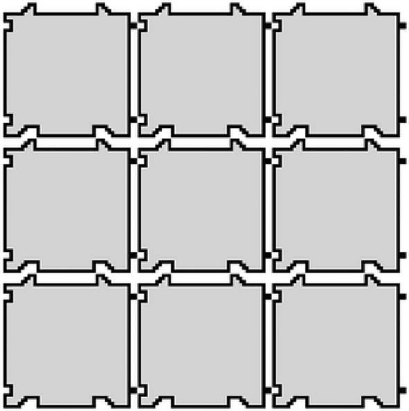
Figure 4. Tiles with matching bumps and dents, forcing their placement on the nodes of a square lattice.
Since the geometrical tiles are placed on the nodes of a square lattice, the notions of geometrical tiling and geometrical tiled path have the same meaning as in the case of Wang tiles.
We say that a geometrical tiling (resp. a geometrical tiled path) is non-overlapping if no two tiles are overlapping. Note that we may refer to non-overlapping tiled paths also as “ribbons”. This is because, similarly to the case of Wang tiles, the underlying path of this construction imposes a quasi-linear neighborhood to all tiles; namely, each tile (except the first and the last, if any) has a predecessor and a successor. Even more, by using standard methods employed in previous papers (see Adleman et al., 2002
, 2009
; Czeizler and Kari, Submitted), one can easily transform such a non-overlapping tiled path into a ribbon of Wang tiles.
In the following sections we show that in the framework of geometric tiles, the notions of non-overlapping tiling and non-overlapping tiled path are equivalent to that of a valid tiling and valid zipper structure, respectively.
The “Tall” Von Neumann Neighborhood Vector “T”
In this section we consider the “tall” von Neumann neighborhood vector from Example 2,
N=((0, 1), (0, 2), (1, 0), (0, −1), (0, −2), (−1, 0)),
which contains six elements, as described more suggestively by the pattern:
Let T ⊆ X6 be a tile system using this neighborhood vector, where X is the set of possible glues of the edges. We design a geometrical tile system G inducing a direct correspondence between valid (partial) T-tilings and T-zippers and non-overlapping G-tilings and G-tiled paths, respectively.
Given a tile t ∈ T, we denote by (tN, tNN, tE, tS, tSS, tW) the ordered set of its glues, instead of (t(0, 1), t(0, 2), t(1, 0), t(0, −1), t(0, −2), t(−1, 0)). Let n be the total number of glues, i.e., |X|=n. For each tile t=(tN, tNN, tE, tS, tSS, tW) ∈ T, we construct n geometric tiles  called the geometrical variants of t. The reason for which we need to introduce multiple geometrical variants for each tile t will be explained in detail later, when we introduce some specific constructions, called the spike, the big dent, and the sheath. The base shape of all geometric tiles is a square. However, on the edges of these squares we place specific bumps and dents in order to simulate the glues of the original tile. We use the East and West edges of the geometric tiles to simulate the glues corresponding to the East and West neighbors. At the same time, the North and South edges are used to simulate the glues corresponding to the four neighbors placed one and two steps to the North and to the South.
called the geometrical variants of t. The reason for which we need to introduce multiple geometrical variants for each tile t will be explained in detail later, when we introduce some specific constructions, called the spike, the big dent, and the sheath. The base shape of all geometric tiles is a square. However, on the edges of these squares we place specific bumps and dents in order to simulate the glues of the original tile. We use the East and West edges of the geometric tiles to simulate the glues corresponding to the East and West neighbors. At the same time, the North and South edges are used to simulate the glues corresponding to the four neighbors placed one and two steps to the North and to the South.We discuss first the East and West edges of the geometrical variants of a given tile t. First, to each glue from X we associate a unique position along the East and the West edges. Then, in all geometrical variants of t we place a bump on the East edges on the unique position associated to the glue tE and a dent on the West edges on the unique position associated to the glue tW, see e.g., Figure 5
. Thus, if the glues of two horizontally adjacent tiles are matching, then the bump and the dent of the corresponding edges of the two associated geometric tiles are placed exactly on the same position, i.e., they fit each other. For example, if the glue on the East edge of a tile t is the same as the glue on the West edge of a tile t′, i.e., tE=t′W, then the bump on the East side of any of the t geometrical variants fits exactly with the dent on the West side of any of the t′ geometrical variants. However, if for two tiles t and t′ we have tE ≠ t′W, then the bump from the East edge of any of the variants of t overlaps with the West edge of any of the variants of t′.
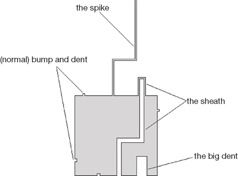
Figure 5. A geometric tile for the case of the “tall” von Neumann neighborhood.
Let us consider now the North and South edges of the geometrical variants of t. The structure of these edges is more complex, as here we use bumps and dents both to communicate with neighboring tiles and to allow the propagation of information. Thus, both edges are split in three regions, and to every glue we associate a unique position in each of these regions.
The first regions of the North and the South edges of the geometrical variants of t are used in order to communicate with the tiles placed immediately to the North and to the South, respectively. Similar to the case of East and West edges, we place a bump on the North edge and a dent on the South edge of each of the variants. The bump on the North edge is placed on the unique position from the first region associated to the glue tN, while the dent on the South edge is placed on the unique position from the first region associated to the glue tS.
The second and the third regions of the North and respectively the South edges of the geometrical variant of t are used to simulate the glues on the virtual edges of t. Thus, on the second region of the North edge of each of the geometrical variants of t we place an elongated bump, called spike. This spike is used to simulate the glue tNN, and thus it is placed (on all geometrical variants) on the unique position from the second region of the North edge associated to it. The spike is long enough to cross the first geometric tile to the North and to reach the South edge of the geometric tile placed two steps to the North. Moreover, the spike shifts its position, see Figure 5
, such that when it reaches the second tile to the North, the spike is placed on the unique position from the third region associated to the glue tNN. If this second geometric tile is a variant of a tile t′ such that t′SS=tNN, then there exists a matching dent in the third region; otherwise an overlap will occur. As previously suggested, on the third region of the South edge of each of the geometrical variants of t we place a wider dent, called the big dent. This big dent is used to simulate the glue placed on the South virtual edge of t, that is tSS, and it is placed (on all geometrical variants of t) on the unique position associated to the glue tSS from the third region of the South edge, see Figure 5
.
Until now, all the geometrical variants of t, that is  have identical shapes. However, the difference between them is given by the sheath which is placed on the second region of the South edge and the third region of the North edge of the geometrical variants. The sheath is a pair of a matching bump and dent, see Figure 5
, which perfectly surrounds the spike of the tile below. Due to this sheath, geometric tiles can propagate information from the tile below, to the tile above. Since there are n different possible positions for the spike of the geometric tile placed below, each of the variants of t will cover for exactly one of these possibilities, see Figure 6
(thus, the required number of different geometrical variants for t). Note that the big dent is constructed wide enough such that it actually matches both the spike (of the tile placed two steps below) and the possible sheath (of the tile placed one steps below) surrounding the spike. In Figure 7
we display a non-overlapping tiling using geometric tiles which is associated to the valid tiling from Figure 1
. Note that the tiling from Figure 7
is only one of the possible non-overlapping tilings which can be associated to the tiling from Figure 1
. For instance, the top right geometric tile can be replaced by any other geometrical variant of the same tile, without causing any overlapping.
have identical shapes. However, the difference between them is given by the sheath which is placed on the second region of the South edge and the third region of the North edge of the geometrical variants. The sheath is a pair of a matching bump and dent, see Figure 5
, which perfectly surrounds the spike of the tile below. Due to this sheath, geometric tiles can propagate information from the tile below, to the tile above. Since there are n different possible positions for the spike of the geometric tile placed below, each of the variants of t will cover for exactly one of these possibilities, see Figure 6
(thus, the required number of different geometrical variants for t). Note that the big dent is constructed wide enough such that it actually matches both the spike (of the tile placed two steps below) and the possible sheath (of the tile placed one steps below) surrounding the spike. In Figure 7
we display a non-overlapping tiling using geometric tiles which is associated to the valid tiling from Figure 1
. Note that the tiling from Figure 7
is only one of the possible non-overlapping tilings which can be associated to the tiling from Figure 1
. For instance, the top right geometric tile can be replaced by any other geometrical variant of the same tile, without causing any overlapping.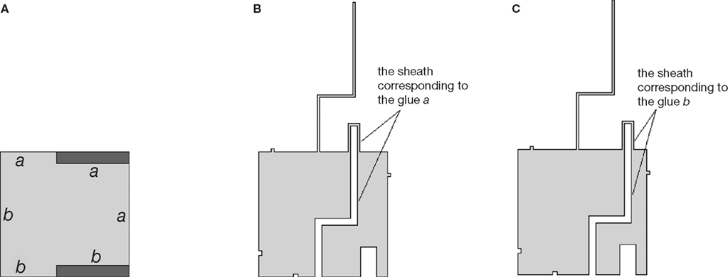
Figure 6. The geometrical variants of a tile, for the case when X={a, b}: (A) the tile, (B) the first geometrical variant, (C) the second geometrical variant.
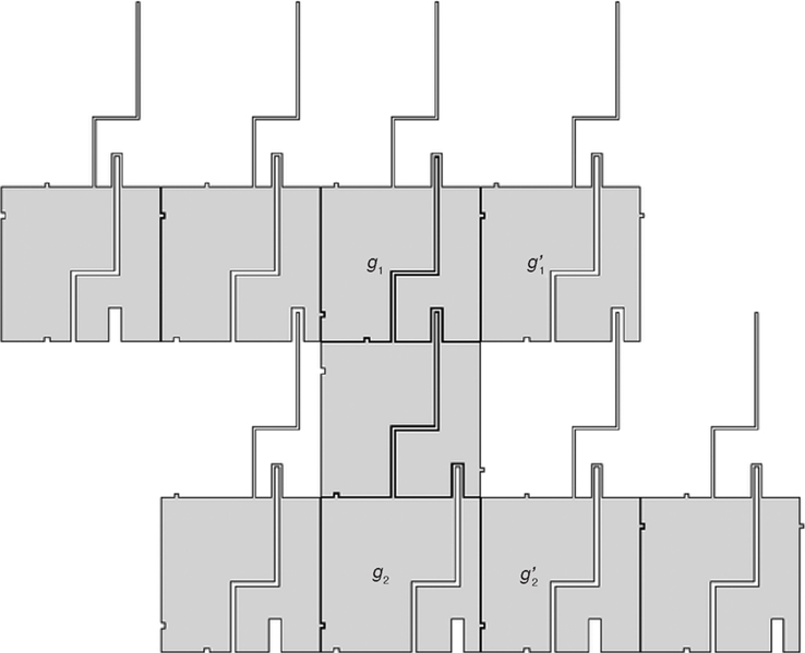
Figure 7. A non-overlapping tiling of geometric tiles, for the case of the “tall” von Neumann neighborhood.
The reason for which we have to use the spike, the big dent, and the sheath instead of using normal (small) bumps and dents is the following. We want each geometric tile to act as an intermediate between the tile below and the tile above. However, we cannot be sure whether given a partial tiling 𝒯D (or similarly a zipper construction) between any two tiles which are placed two steps North of each other, there is also a third tile placed in between. That is, even if (x, y), (x, y + 2) ∈ D, it is not necessary that (x, y + 1) ∈ D. Thus, we must make sure that in both cases, i.e., whether there exists or not a middle tile t(x, y + 1), the information regarding the glue t(x, y)NN is transferred from t(x, y) to t(x, y + 2). In our case, this is accomplished by the matching spikes, big dents, and sheaths; see for example the tiles g1 and g2 from Figure 7
for the case when there is a tile in between, and the tiles g′1 and g′2 for the other case.
Observation 1: both the spike and the sheath have a step-like form due to the following reason. We design the geometric tiles such that all of them have the same square base shape, up to the positions of their bumps and dents along their edges (including here also the spike, the big dent, and the sheath). Thus, if we would have chosen the spike (and hence also the sheath) to have a straight form then, the spike, the big dent, and the sheath, would all be placed in the same region of the South and the North edges of a geometric tile. Thus, for instance, in the case when for some tile t(x, y) we have t(x, y)SS=t(x, y)NN then, in all the geometrical variants of t(x, y), the spike and the big dent will actually overlap with each other. Even more, in that particular geometric variant of this tile, t(x, y), in which also the sheath corresponds to the glue t(x, y)SS, the spike and the big dent are going to overlap also with the sheath, making the construction much more complicated. Also, in many other cases, the spike and the sheath of a geometrical tile placed on position (x, y) will overlap with the spike, the big dent and the sheath of the geometrical tile placed on position (x, y + 1). Although such a design is not impossible, by allowing the spike and the sheath to have a step-like shape we overcome all of these overlapping problems.
Theorem 1: let N=((0, 1), (0, 2), (1, 0), (0, −1), (0, −2), (−1, 0)) be a neighborhood vector, and let T ⊆ X6 be a tile system using this neighborhood. Then, we can construct a geometrical tile system G such that for any surface D ⊆ ℤ2, there exists a one-to-one correspondence between valid 𝒯D-tilings and non-overlapping 𝒢D-tilings, up to replacing some of the tiles with any of its geometrical variants.
Proof: Let 𝒯D : D → T be a valid tiling, and let G be a geometrical tile system constructed as described above. Then, for each (x, y) ∈ D we replace the tile t(x, y) with one of its geometrical variants as follows:
• If (x, y − 1), (x, y + 1) ∉ D, then we replace t(x, y) with any of its geometrical variants.
• If either (x, y − 1) ∈ D or (x, y + 1) ∈ D, then we replace t(x, y) with the geometrical variant whose sheath matches either the spike of the geometric tile below or the big dent of the geometric tile above, respectively. Note that independently of which geometrical variants of the tile below and the tile above we use, the spike and the big dent are the same.
• If both (x, y − 1), (x, y + 1) ∈ D, then we replace t(x, y) with the geometrical variant whose sheath matches the spike of the geometric tile below. Since the tiling 𝒯D is valid, we must have t(x, y − 1)NN=t(x, y + 1)SS. Thus, the sheath of the chosen geometrical variant also matches the big dent of the geometric tile above.
In all of the above cases we do not obtain any overlapping between the spikes, big dents, and sheaths of the geometric tiles. Moreover, since we assumed the tiling 𝒯D to be valid, we also conclude that there is no overlapping between the normal bumps and dents of all adjacent geometric tiles. Thus, the tiling 𝒢D : D → G obtained by replacing the tiles from T with the corresponding geometric tiles from G as described above, is non-overlapping. Moreover, except for the first case mentioned above, i.e., for some (x, y) ∈ D, both (x, y − 1), (x, y + 1) ∉ D, where we can replace the tile t(x, y) with any of its geometrical variants, on all the other cases each tile can be replaced only by one of its geometrical variants.
For the converse, let us assume that 𝒢D : D → G is a non-overlapping tiling. From the definition of the geometric tile system G, each geometric tile from 𝒢D is a variant of a (unique) tile in T. We construct the tiling 𝒯D : D → T by replacing each tile from 𝒢D with the corresponding tile from T. Since there are no overlaps in 𝒢D between bumps and dents and also between the spikes and the big dents, we conclude that any tile from 𝒯D must agree on its glues with all of its neighbors from the domain D. Thus, the tiling 𝒯D is valid, and it is uniquely obtained starting from the tiling 𝒢D.□
The conceptual difference between a zipper and a partial tiling is given only by the presence of a path. Moreover, since in both generalized Wang tile systems and geometrical tile systems the tiles are placed on the nodes of a square lattice (actually the same square lattice), the notion of path remains unchanged. Thus, the following result is a direct consequence of the previous theorem.
Corollary 1: let N=((0, 1), (0, 2), (1, 0), (0, −1), (0, −2), (−1, 0)) be a neighborhood vector, and let T ⊆ X6 be a tile system using this neighborhood. Then, we can construct a geometrical tile system G such that for any non self-crossing path P there exists a one-to-one correspondence between T-zippers (P, r) and non-overlapping G-tiled paths (P, s), up to replacing some of the tiles with any of its geometrical variants.
The f-Neighborhood Vector “ƒ”
In this section we consider the neighborhood vector
N=((0, 1), (0, 2), (1, 2), (1, 0), (0, −1), (0, −2), (−1, −2), (−1, 0)),
which contains eight elements and is described by the following pattern:
This neighborhood describes the shape of the letter f and it is obtained by adding to the “tall” von Neumann neighborhood vector from the previous section the two symmetric elements (1, 2) and (−1, −2). The geometric tiles which we use in this case are obtained by adding to the previous geometric tiles a new pair of matching spikes, big dents and sheaths, which are used to send, receive and respectively transfer the information from a given tile to the one corresponding to the relative position (1, 2).
The new spike, called spike II, is placed along the East edge of the geometric tiles, and it points upwards, see Figure 8
. This structure is used to simulate the glue corresponding to the virtual edge which links a tile to its neighbor placed on the relative position (1, 2). Contrary to the case of the first spike, the starting point of the spike II is the same, independently of which glue it stands for. However, the length of its first horizontal segment uniquely determines which glue it simulates. Before spike II reaches the South edge of the tile placed on the relative position (1, 2) it crosses both the tile placed on the relative position (1, 0) and the tiled placed on the relative position (1, 1). Thus, we construct two new sheaths, called sheath II and sheath III, which enable the crossing of spike II through these two tiles, without overlapping.
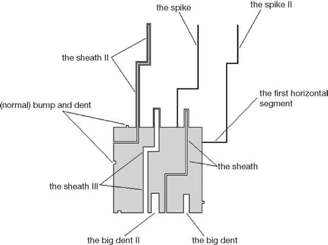
Figure 8. A geometric tile for the case of the f-neighborhood.
The new big dent, called big dent II, is placed on the South edge of the geometric tiles, and it corresponds to the glue of the virtual edge which connects a tile to its neighbor placed on the relative position (−1, −2). Thus, it has to match the spike II of the geometric tile placed on this position. In fact, as we explain next, it has to match both the spike II and the corresponding sheaths surrounding it: the sheath II of the geometric tile placed on the relative position (0, −2), and the sheath III of the geometric tile placed on the relative position (0, −1).
The sheath II starts from the West edge of the geometric tiles and it surrounds the spike II of the geometric tile to the left, i.e., the tile placed on the relative position (−1, 0). Thus, the sheath II crosses the geometric tile placed above it [i.e., the tile placed on the relative position (1, 0)], resembling in some sense a spike.
The sheath III starts from the South edge of the geometric tiles and it surrounds both the spike II of the geometric tile placed on the relative position (−1, −1) and the sheath II of the geometric tile placed on the relative position (0, −1) (which itself also surrounds the spike II).
For a better understanding of these constructions and how they embed in each other, in Figure 9
we present a partial non-overlapping tiling using these geometric tiles. As explained in Observation 1, all these constructions, i.e., the spike II, the sheath II, and the sheath III, must have a step-like form in order to avoid overlapping with similar structures from the surrounding geometric tiles. Thus, some new splitting of the edges are necessary as follows. The East and West edges are split into two regions, while the South and North edges are split into five (two new regions are created on the left side of the edges).
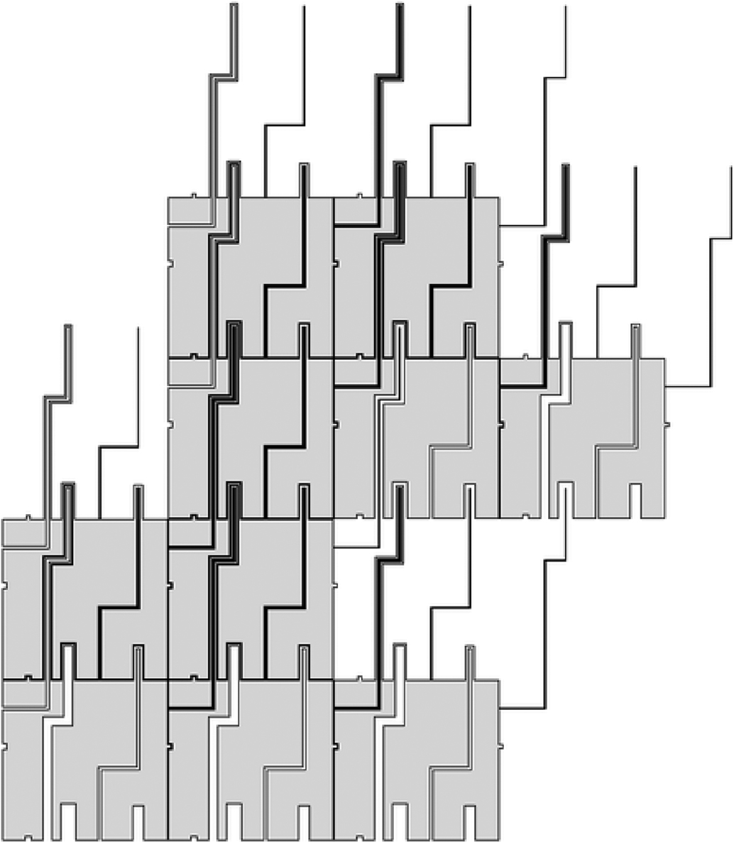
Figure 9. A non-overlapping tiling of geometric tiles, for the case of the f-neighborhood.
The spike II starts from the upper region of the East edge. As previously mentioned, the starting position of this construction (along the edge) is independent of the glue it stands for. However, the length of the first horizontal segment of spike II is unique for each of the n different glues. Thus, the first vertical segment of the spike II reaches the second region of the South edge of the tile placed on the relative position (1, 1) on the unique position associated to the glue simulated by spike II. Before reaching the South edge of the tile placed on the relative position (1, 2), the spike II shifts again, such that now it intersects the edge on the third region (again on the unique position corresponding to the same specific glue).
The sheath II must surround the spike II of the tile on the left. Thus, it starts from the upper region of the West edge, it shifts horizontally, it crosses the second region of the South edge of the tile above, and, after shifting again, it reaches the third region of the South edge of the tile placed on the relative position (0, 2). Note that the positions from both the second region of the South edge of the tile above and the third region of the South edge of the tile two steps above in which the sheath II crosses these tiles, must correspond to the same glue.
The sheath III starts from the second region of the South edge, it shifts once, and it reaches the third region of the South edge of the tile above. Also in this case, the position from the second region of the South edge on which it starts must correspond to the same glue as the position reached on the third region of the South edge of the tile above.
In order to make the transition from tiles with glues to geometric tiles, we proceed as follows. Given a tile system T ⊆ X8, for each tile t ∈ T we construct n3 geometrical variants, where n=|X| is the number of distinct glues. All these n3 geometrical variants of t have the same bumps, dents, spikes and big dents. This is because all these structures simulate the eight glues of the tile t, and they are all placed on the exact position corresponding to the particular glues they simulate. However, on distinct geometric variants, the sheaths must be placed on different positions along the specific regions of the edges. This is due to the fact that the sheaths have the role of allowing the crossing of spikes from a neighboring geometric tile to another, without overlapping. Thus, since these spikes can be placed on n different places along the edges (or actually along one particular region of the edges), for each tile t there must exist a geometric variant corresponding to each of these n cases. Since there are three sheaths, for each tile we must have n3 geometric variants.
Theorem 2: let
N=((0, 1), (0, 2), (1, 2), (1, 0), (0, −1), (0, −2), (−1, −2), (−1, 0))
be a neighborhood vector, and let T ⊆ X8 be a tile system using this neighborhood. Then, we can construct a geometrical tile system G such that for any surface D ⊆ ℤ2, there exists a one-to-one correspondence between valid 𝒯D-tilings and non-overlapping 𝒢D-tilings, up to replacing some of the tiles with several of its geometrical variants.
Proof: Let 𝒯D : D → T be a valid tiling, and let G be a geometrical tile system constructed as described above. Then, for each (x, y) ∈ D we replace each tile t(x, y) with one of its geometrical variants. Since the sheaths of the geometric tile g(x, y) are coming in contact with the geometric tiles on positions (x − 1, y), (x − 1, y − 1), (x, y − 1), (x, y + 1), (x, y + 2) (if these positions are in the domain D), we must select carefully which geometrical variant of t(x, y) we should use. Depending on whether or not one or several of the five positions mentioned above are in the domain of the tiling 𝒯D, we make the following choices (we describe here just three situations, the others cases being very similar):
• If (x − 1, y), (x − 1, y − 1), (x, y − 1), (x, y + 1), (x, y + 2) ∉ D, then we can replace t(x, y) with any of its geometrical variants. This is because all the sheaths of the geometric tile g(x, y) are not coming in contact with any other geometric tile.
• If (x, y + 2) ∈ D or (x − 1, y) ∈ D (or both) then we replace t(x, y) with its geometrical variant whose sheath II corresponds to the glue t(x, y + 2)(−1, −2) or t(x − 1, y)(1, 2), respectively. Note that if both (x, y + 2), (x − 1, y) ∈ D then, since the tiling 𝒯D is valid, it must be that t(x, y + 2)(−1, −2)=t(x − 1, y)(1, 2).
• If (x, y + 1) ∈ D then we replace t(x, y) with its geometrical variant which satisfies the following conditions. First, its sheath should correspond to the glue t(x, y + 1)(0, −2). Then, its sheath II should be perfectly surrounded by the sheath III of the geometric tile above (here, there may be several variants having this property). If also (x, y + 2) ∈ D, then the sheath II should correspond to the glue t(x, y + 2)(−1, −2). Finally, its sheath III should correspond to the glue t(x, y + 1)(−1, −2).
The other cases are treated in a similar manner.
By choosing the correct geometrical variants for the tiles, since the tiling 𝒯D is valid, we do not obtain any overlapping in 𝒢D. Thus, the tiling 𝒢D : D → G obtained by replacing the tiles from T with the corresponding geometric tiles from G as described above, is non-overlapping. Moreover, the tiling 𝒢D is unique, up to replacing some of its geometrical tiles with other geometrical variant of the same tile.
For the converse, if 𝒢D : D → G is a non-overlapping tiling then, just as in the previous section, we construct the tiling 𝒯D : D → T by replacing each tile from 𝒢 with the corresponding tile from T (each tile in G is a geometrical variant of a unique tile from T). Since there is no overlapping in 𝒢D between bumps and dents and also between the spikes and the big dents, we conclude that any tile from 𝒯D must agree on its glues with all of its neighbors from the domain D. Thus, the tiling 𝒯D is valid, and it is uniquely obtained starting from the tiling 𝒢D.□
As in the previous section, the following result is an immediate consequence.
Corollary 2: let
N=((0, 1), (0, 2), (1, 2), (1, 0), (0, −1), (0, −2), (−1, −2), (−1, 0))
be a neighborhood vector, and let T ⊆ X8 be a tile system using this neighborhood. Then, we can construct a geometrical tile system G such that for any non self-crossing path P there exists a one-to-one correspondence between T-zippers (P, r) and non-overlapping G-tiled paths (P, s), up to replacing some of the tiles with several of its geometrical variants.
The 3 × 5 “Filled” Rectangular Neighborhood Vector
As a final case, we consider the neighborhood vector N containing 14 positions, which is described by the following pattern:
In this case, the neighbors of a tile t(x, y) are all the tiles contained in the 3 × 5 rectangle centered on (x, y), except for (x, y). The geometric tiles used in this case are obtained by combining several geometrical tile designs. We combine the geometrical tile design given in the previous section with its symmetric design, and also with a new tile design which is described below.
In Czeizler and Kari (Submitted) we present a motif construction of a certain shape, which is used for proving that a tiling using the Moore neighborhood, see Example 3, can be simulated by another tiling using a quasi linear neighborhood, i.e., a partial von Neumann neighborhood. This shape is obtained by attaching a square to a regular hexagon and by placing several bump and dent constructions on its edges, see Figure 10
A. This motif construction can be used for designing a geometrical tile system which can simulate the tiles with glues having the Moore neighborhood. As in the case of the geometric tiles presented in the previous sections, between the bump and dent constructions of these geometric tiles we can distinguish a spike, a big dent and a sheath. Note that this shape, i.e., a square attached to a regular hexagon, can indeed tile the plane, as it is derived from one of the 11 Archimedean Tilings done by regular polygons (see Grünbaum and Shephard, 1987
). In Figure 10
B we present one of the non-overlapping tilings by geometric tiles which is associated to the tiling from Figure 2
.
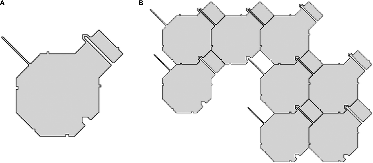
Figure 10. Geometric tiles for the case of the Moore neighborhood: (A) a geometric tile; (B) one of the non-overlapping tilings by geometric tiles which can be associated to the tiling from Figure 2
.
By putting together all of these constructions, we obtain a geometrical tile design which has three pairs of normal (small) bumps and dents, four spikes, four big dents, and six sheaths. In Figure 11
we present both the design of these geometric tiles as well as a non-overlapping tiling obtained using this geometrical tile system (the small bumps and dents are omitted from the pictures). Note also that since in this case we have six sheaths, for each tile we have to construct n6 geometrical variants, where n=|X| is the number of glues.
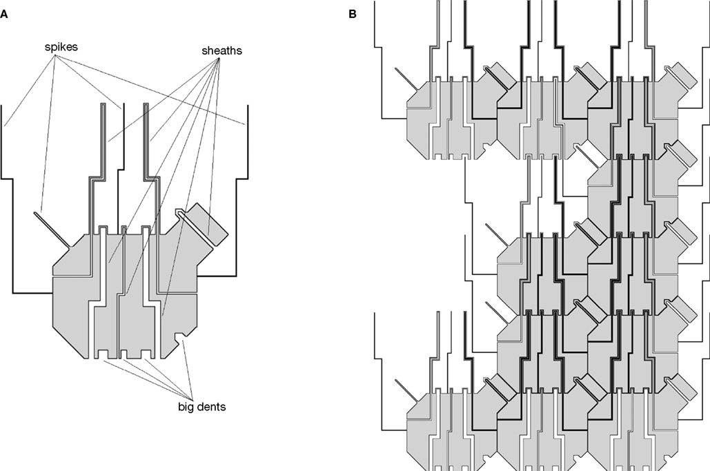
Figure 11. Geometric tiles for the case of the 3 × 5 “filled” rectangular neighborhood (normal bumps and dents are omitted): (A) a geometric tile; (B) a non-overlapping tiling by geometric tiles.
Theorem 3: let N be the 3 × 5 “filled” rectangular neighborhood vector, and let T ⊆ X14 be a tile system using this neighborhood. Then, we can construct a geometrical tile system G such that for any surface D ⊆ ℤ2, there exists a one-to-one correspondence between valid 𝒯D-tilings and non-overlapping 𝒢D-tilings, up to replacing some of the tiles with several of its geometrical variants.
Corollary 3: let N be the 3 × 5 “filled” rectangular neighborhood vector, and let T ⊆ X14 be a tile system using this neighborhood. Then, we can construct a geometrical tile system G such that for any non self-crossing path P there exists a one-to-one correspondence between T-zippers (P, r) and non-overlapping G-tiled paths (P, s), up to replacing some of the tiles with several of its geometrical variants.
In this paper we showed how to simulate partially-tiled paths (zippers) that use square tiles with complex neighborhood relations, by ribbons of geometrical tiles that use a very simple, local neighborhood relation based solely on non-overlapping. We namely solved this problem for the case of the “tall” von Neumann neighborhood (a slightly “taller” version of the von Neumann cross-shaped neighborhood), the f-shaped neighborhood, and the 3 × 5 “filled” rectangular neighborhood.
The techniques we used can be extended to some other particular cases of neighborhoods. For instance, the method from Section “The ‘Tall’ von Neumann Neighborhood Vector ‘┼’” can be easily extended for the case when the von Neumann neighborhood’s vertical arm is arbitrarily tall, i.e., the neighborhood contains one or several pairs of the form (0, k), and their symmetric ones (0, −k), where k ≥ 2. These positions correspond to those tiles placed k-steps to the North and to the South. For each such new position (0, k) and its symmetric (0, −k), we have to add a new spike, big dent, and k − 1 sheaths on the North and South edges. The spike has to be sufficiently long, i.e., a little longer than (k − 1)-times the size of the East edge, while the lengths of the sheaths would have to match the spike, i.e., decreasing from (k − 1)- to one-times the length of the East edge. Also, all these structures would have to be in a step like form, in order not to overlap with the similar structures from the above and below tiles.
By generalizing the methods described in Section “The f-Neighborhood Vector ‘ƒ’”, we can further extend the “arbitrarily tall” von Neumann neighborhood of the previous paragraph by adding to it pairs of the form (1, k) or (−1, k), and their symmetric ones (−1, −k) and (1, −k), respectively, where k ≥ 2. Here, for each new position (1, k) and the symmetric one (−1, −k), we add one spike starting from the East edge, one big dent on the South edge, one sheath on the West and North edges, and k − 1 sheaths on the South and North edges.
By putting together all the above considerations, we conclude the following. Let Nk and  be the neighborhoods Nk={(i,j)|−1 ≤ i ≤ 1,−k ≤ j ≤ k, and (i,j) ≠ (0,0)} and
  Informally, this neighborhood is a rectangular Moore-type neighborhood, centered at the tile of reference, and with width 3 and height 2k + 1 (or height 3 and width 2k + 1). Then, for all tile systems TN, were N is a symmetric neighborhood which can be included in one of the above neighborhoods, i.e., such that there exists k ≥ 0 with
  or
or  we can design a geometrical tile system G such that any (partial) T-tiling or T-zipper can be simulated by a non-overlapping G-tiling or G-tiled path, respectively. Note that such a neighborhood included in a 3 × (2k + 1) rectangle need not be contiguous, i.e., may even have holes in it. On the other hand, we observe that an immediate generalization of the previous techniques cannot be directly applied to the case of completely arbitrary neighborhoods [not even for neighborhoods included in a 5 × (2k + 1) rectangle], since the spikes and sheaths we would have to add in these cases would self-overlap.
be the neighborhoods Nk={(i,j)|−1 ≤ i ≤ 1,−k ≤ j ≤ k, and (i,j) ≠ (0,0)} and Informally, this neighborhood is a rectangular Moore-type neighborhood, centered at the tile of reference, and with width 3 and height 2k + 1 (or height 3 and width 2k + 1). Then, for all tile systems TN, were N is a symmetric neighborhood which can be included in one of the above neighborhoods, i.e., such that there exists k ≥ 0 with or we can design a geometrical tile system G such that any (partial) T-tiling or T-zipper can be simulated by a non-overlapping G-tiling or G-tiled path, respectively. Note that such a neighborhood included in a 3 × (2k + 1) rectangle need not be contiguous, i.e., may even have holes in it. On the other hand, we observe that an immediate generalization of the previous techniques cannot be directly applied to the case of completely arbitrary neighborhoods [not even for neighborhoods included in a 5 × (2k + 1) rectangle], since the spikes and sheaths we would have to add in these cases would self-overlap.The authors declare that the research was conducted in the absence of any commercial or financial relationships that could be construed as a potential conflict of interest.