1
NORDITA, Stockholm, Sweden
2
Department of Computational Biology, AlbaNova University Centre, Stockholm, Sweden
3
ACCESS Linnaeus Centre, KTH-Royal Institute of Technology, Stockholm, Sweden
4
The Niels Bohr Institute, Copenhagen University, Copenhagen, Denmark
Statistical models for describing the probability distribution over the states of biological systems are commonly used for dimensional reduction. Among these models, pairwise models are very attractive in part because they can be fit using a reasonable amount of data: knowledge of the mean values and correlations between pairs of elements in the system is sufficient. Not surprisingly, then, using pairwise models for studying neural data has been the focus of many studies in recent years. In this paper, we describe how tools from statistical physics can be employed for studying and using pairwise models. We build on our previous work on the subject and study the relation between different methods for fitting these models and evaluating their quality. In particular, using data from simulated cortical networks we study how the quality of various approximate methods for inferring the parameters in a pairwise model depends on the time bin chosen for binning the data. We also study the effect of the size of the time bin on the model quality itself, again using simulated data. We show that using finer time bins increases the quality of the pairwise model. We offer new ways of deriving the expressions reported in our previous work for assessing the quality of pairwise models.
In biological networks the collective dynamics of thousands to millions of interacting elements, generating complicated spatiotemporal structures, is fundamental for the function. Until recently, our understanding of these structures was severely limited by technical difficulties for simultaneous measurements from a large number of elements. Recent technical developments, however, are making it more and more common that experimentalists record data from larger and larger parts of the system. A living example of this story is what is now happening in Neuroscience. Until a few years ago, neurophysiology meant recording from a handful of neurons at a time when studying early stages of sensory processing (e.g. the retina), and only single neurons when studying advanced cortical areas (e.g. inferotemporal cortex). This limit is now rapidly going away, and people are collecting data from larger and larger populations (see e.g. the contributions in Nicolelis, 2007
). However, such data will not help us understand the system per se. It will only give us large collections of numbers, and most probably we will have the same problem that we had with the system, but now with the data set: we can only look at small parts of it at a time, without really making use of its collective structures. To use such data and make sense of it we need to find systematic ways to build mathematically tractable descriptions of the data, descriptions with lower dimensionality than the data itself, but involving relevant dimensions.
In recent years, binary pairwise models have attracted a lot of attention as parametric models for studying the statistics of spike trains of neuronal populations (Schneidman et al., 2006
; Shlens et al., 2006
, 2009
; Tang et al., 2008
; Roudi et al., 2009a
,b
), the statistics of natural images (Bethge and Berens, 2008
), and inferring neuronal functional connectivities (Shlens et al., 2006
; Yu et al., 2008
). These models are the simplest parametric models that can be used to describe correlated neuronal firing. To build them one only needs the knowledge of the distribution of spike probability over pairs of neurons, and, therefore, these models can be fit using reasonable amounts of data. When dealing with statistical models, there are two main questions that one needs to answer. The first question is the inference question, i.e. how one can find the best parameters for the model given the data. The second question is the question of model quality, i.e. once the best parameters are found, how good the fitted model is for describing the statistics of the data. These questions can be naturally studied in the framework provided by statistical physics. Starting from a probability distribution over the states of a number of elements, statistical physics deals with computing quantities such as correlation functions, entropy, free energy, energy minima, etc., through exact or carefully developed approximate methods. It allows one to give quantitative answers to questions such as: what is the entropy difference between real data and the parametric model? Is there a closed-form equation relating model parameters to the correlation functions? How well does a pairwise model approximate higher order statistics of the data?
This paper has three main purposes: (a) to provide a summary of the previous results, derived using statistical physics, on the parameter inference and quality of pairwise models, (b) to study how the choice of the time bin size affects the inference and model quality problems and, (c) to report new and somewhat simpler derivations of our previous results.
In building binary pairwise models a crucial step is binning the spike trains into small time bins and assigning −1 or 1 to each bin depending on whether there is a spike in it or not. The answers to the inference and model quality problems may thus be affected by the choice of this time bin size. In what follows, we first deal with the effect of the size of the time bin on the answer of the inference question. We review a number of approximate methods described in Roudi et al. (2009b)
for inferring the parameters of the pairwise model and study how their quality depends on the choice of the bin size. We also describe a new approximation, the independent-triplet (IT) approximation, as an extension to the independent-pair (IP) approximation described in Roudi et al. (2009b)
. We show that although IT slightly outperforms IP, it cannot beat the more powerful approximations that we describe, i.e. the Thouless–Anderson–Palmer (TAP) inversion, and the Sessak–Monasson (SM) approximation. We also derive the TAP inversion approximation from the celebrated Belief Propagation algorithm. After this, we study the effect of the size of the time bin on the answer to the model quality question. This issue has been studied analytically in Roudi et al. (2009a)
, using a perturbative expansion. They derived equations for the difference between the entropies of the pairwise model and the true distribution of the data, as well as between an independent-neuron model and the data, when  (the so called “perturbative regime” or the “low-rate regime”). Here, N is the number of neurons,
  is the average firing rate and δt is the size of the time bin. They concluded that the quality of the pairwise model increases by decreasing δt or N. In this paper, we confirm these analytical results on data generated from a model cortical network.
(the so called “perturbative regime” or the “low-rate regime”). Here, N is the number of neurons, is the average firing rate and δt is the size of the time bin. They concluded that the quality of the pairwise model increases by decreasing δt or N. In this paper, we confirm these analytical results on data generated from a model cortical network.A crucial step in the derivation of entropy differences in Roudi et al. (2009a)
was to express the pairwise distribution in the so called Sarmanov–Lancaster representation (Lancaster, 1958
; Sarmanov, 1963
). Here we show that one can derive the same expressions by approximating the partition function of a Gibbs distribution (Eq. 2 in Section “The Binary Pairwise Model”). In addition to recovering the low-rate expansion of the entropies, we use the results to find the difference between the probability of synchronous spikes according to the true distribution, the pairwise model and the independent model. We also show that one can derive the results of Roudi et al. (2009a)
by extending the idea behind the IP approximation to triplets of neuron, i.e. the IT approximation. By taking the limit νiδt → 0 of the IT approximation to the entropy of a given distribution, where νi is the firing rate of the ith neuron, we show that the results of Roudi et al. (2009a)
can be recovered in a considerably simpler way.
In the last part of the paper, we discuss two possible extensions of the binary pairwise models and mention a number of important questions that they raise. We first describe the extensions to non-binary variables useful for studying the statistics of modular models of cortical networks. We then describe an extension of the pairwise model to a model with asymmetric connections which gives promising results for discovering the synaptic connectivity from neural spike trains.
The Binary Pairwise Model
In a binary pairwise model, starting from the spikes recorded from N neurons, one first divides the spike trains into small time bins. One then builds a binary representation of the spike trains by assigning a binary spin variable si(t) to each neuron i and each time bin t, with si(t) = −1 if neuron i has not emitted any spikes in that time bin, and si(t) = −1 if it has emitted one spike or more. From this binary representation, the mean values and correlations between the neurons are computed as
where T is the total number of time bins.
The binary pairwise model of the data is then built by considering the following distribution over a set of N binary variable s = (s1,s2,…,sN)

and choosing the parameters, hi and Jij such that the mean values and pairwise correlations under this distribution matches those of the data defined in Eq. 1, that is
Following statistical physics terminology, the parameters hi are usually called the external fields and Jij, the pairwise couplings or pairwise interactions. One important property of the pairwise distributions in Eq. 2 is that it has the maximum amount of entropy among all the distribution that have the same mean and pairwise correlations as the data, and it is thus usually called the maximum entropy pairwise model. It is also called the Ising model, in accordance with the Ising model introduced in statistical physics as a simple model of magnetic materials.
Although typically written in terms of ±1 spin variables, it is sometimes useful to write the pairwise distribution of Eq. 2 in terms of Boolean variables ri = (si + 1)/2. In the rest of the paper, we sometimes use such Boolean representation as some of the calculations and equations become considerably simpler in this representation. We denote the external fields and the couplings in the Boolean representations by ℋi and 𝒥ij.
The external fields and pairwise couplings can be found using both exact and approximate methods as discussed in details in Roudi et al. (2009b) and reviewed briefly in the following sections. Before reviewing these methods, we first review the experimental studies that have used the maximum entropy pairwise model to study the statistics of spike trains.
The maximum entropy pairwise model as a model for describing the statistics of neural firing patterns was introduced in Schneidman et al. (2006) and Shlens et al. (2006)
. This work used the Ising model to study the response of retinal ganglion cells to natural movies (Schneidman et al., 2006
), steady spatially uniform illumination and white noise (Shlens et al., 2006
), as well as the spontaneous activity of cultured cortical networks (Schneidman et al., 2006
). The main goal of these studies was to find out how close the fitted pairwise model is to the true experimentally computed distribution over s.
As a measure of distance, these studies compared the entropy difference between the true distribution and the pairwise model and compared it with the entropy difference between the true distribution and an independent model. The independent model is a distribution that has the same mean as the data but assumes the firing of each neuron is independent from the rest, i.e.
The measure of misfit can thus be defined as
where the overline indicates averaging with respect to many samples of N neurons. The results of Schneidman et al. (2006)
showed that for populations of size N = 10 or so, Δ was around 0.1. In other words, in terms of entropy difference, the pairwise model offered a ten fold improvement over the independent model. In the other study, Shlens et al. (2006)
found Δ ∼ 0.01 for N = 7. These authors also considered a slightly different model in which only the pairwise correlation between the adjacent cells was used in the fit, and correspondingly the pairwise interactions between non-adjacent cells were set to 0. The results showed that this adjacent pairwise model also performed very well, with Δ ∼ 0.02 on average. It is important to note that in Schneidman et al. (2006)
the stimulus induced long range correlations between cells, while in the data studied Shlens et al. the correlations extended only to nearby cells. Following these studies, Tang et al. (2008)
reproduced these observations to a large extent in other cortical preparations and also concluded that the pairwise model can successfully approximate the multi-neuron firing patterns. In a very recent study (Shlens et al., 2009
), Shlens et al. extended their previous analysis to population of up to 100 neurons concluding that the adjacent pairwise model performs very well even in this case, with Δ ∼ 0.01–0.02. The studies of Shlens et al. were done without stimulation or with white noise stimulus, situations in which neurons do not exhibit strong long range correlations. It is still unclear, from the existing experimental data, how the pairwise models of large size. (not necessarily adjacent) will perform for cases in which neuronal correlations exist between neurons separated by large distance, i.e. when stimulated by natural scenes.
The assumption that Δ is a good measure of distance rests upon the assumption that we are interested in finding out how different the true and model distributions are over the whole space of possible spike patterns. This can be appreciated when we note that the definition in Eq. 5 is equivalent to Δ = DKL(ptrue || ppair)/DKL(ptrue || pind), where DKL(p || q) is the Kullback–Leibler divergence between two distributions p(s) and q(s) defined as DKL(p || q) = Σs p(s)log[p(s)/q(s)]. Using this observation, we can think of Δ as a weighted sum of the difference between the log probability of states according to the true distribution and according to the model distribution normalized by the distance to the independent model. Of course, we may not be interested in finding how different the two distributions are over the space of all possible states, but only how differently the model and true distributions assign probabilities to a subset of important states. For instance, in a particular setting, it may be important only to build a good model for the probability of all states in which some large number of neurons M fire simultaneously (i.e. when Σiri = M), regardless of how different the two distribution are on the rest of the states. It was found in Tkacik et al. (2006)
that the pairwise model offers a significant improvement over the independent model in modelling the experimental probability of synchronous multi-neuron firing of up to N = 15 neurons.
The commonly used Boltzmann Learning algorithm for fitting the parameters of the Ising model is a very slow process, particularly for large N. Although effort has been made to speed up the Boltzmann learning algorithm (Broderick et al., 2007
), such modified Boltzmann algorithms still require many gradient descent steps and long Monte Carlo runs for each step. This fact motivates the development of fast techniques for calculating the model parameters which do not rely on gradient descent or Monte Carlo sampling. A number of such approximations have been studied in Roudi et al. (2009b)
. In what follows we describe these approximations, and in particular the relation between the simpler approximations [naive mean-field (nMF) approximation and the IP approximation] to the more advanced ones (TAP approximation and SM approximation).
Naive Mean-Field Approximation and the Independent-Pair Approximations
The simplest method (Kappen and Rodriguez, 1998
; Tanaka, 1998
) for finding the parameters of the Ising models from the data uses mean-field theory:

where mi = 〈si〉data. These equations express the effective field that determines the magnetization mi as the external field plus the sum of the influences of other spins through their average values mj, weighted by the couplings Jij. Differentiating with respect to a magnetization mj gives the inverse susceptibility (i.e. inverse correlation) matrix

for i ≠ j, where Cij = 〈sisj〉data − mimj. Thus, if one knows the mean values mi and correlations Cij of the data, one can use Eq. 7 to find the Jij and then solve Eq. 6 to find the hi. We call this approximation “naive” mean-field theory (abbreviated nMFT) to distinguish it from the TAP approximation described below, which is also a mean-field theory.
In the IP approximation, one solves the two-spin problem for neurons i and j, ignoring the rest of the network. This yields the following expressions for the parameters in terms of the mean values and correlations:
where  is the external field acting on i when it is considered in a pair with j. It has been noted in Roudi et al. (2009b)
that in the limit mi → −1 and mj → −1,
is the external field acting on i when it is considered in a pair with j. It has been noted in Roudi et al. (2009b)
that in the limit mi → −1 and mj → −1,  matches the leading order of the low-rate expansion derived in Roudi et al. (2009a)
.
matches the leading order of the low-rate expansion derived in Roudi et al. (2009a)
.
is the external field acting on i when it is considered in a pair with j. It has been noted in Roudi et al. (2009b)
that in the limit mi → −1 and mj → −1, matches the leading order of the low-rate expansion derived in Roudi et al. (2009a)
.Although the couplings found in the IP approximation can be directly used as an approximation to the true values of Jij, relating the fields  found from the IP approximation to those of the model is slightly tricky. The reason is that the expression we find depends on which j we took to pair with neuron i. It is natural to think that we can sum
  over j, i.e. over all possible pairings of cell i, to find the Ising model parameter hi. In doing so, however, we should be careful. The expression in Eq. 8b has two types of terms, those that only depend on i, i.e. the first term in the following decomposition, and those that involve j, i.e. the second and third terms below
found from the IP approximation to those of the model is slightly tricky. The reason is that the expression we find depends on which j we took to pair with neuron i. It is natural to think that we can sum over j, i.e. over all possible pairings of cell i, to find the Ising model parameter hi. In doing so, however, we should be careful. The expression in Eq. 8b has two types of terms, those that only depend on i, i.e. the first term in the following decomposition, and those that involve j, i.e. the second and third terms below
The first terms is the field that would have been acting on i if it were not connected to any other neuron, and the rest are contributions from interactions with j. By simply summing  over j, we will be overcounting this term, once for each pairing. In other words, the correct IP approximation for hi will be
over j, we will be overcounting this term, once for each pairing. In other words, the correct IP approximation for hi will be
Although simple in its derivation and intuition, in the limit mi → −1 for all i, Eq. 10 recovers both the leading term and the first order corrections of the low-rate expansion, as shown in Section “The Independent-pair Approximation for the External Fields in the Limit δ → 0” in Appendix.
The simple nMF and IP approximations have been shown to perform well in deriving the parameters of the Ising model when the population size is small.
In Roudi et al. (2009b)
, we showed that for data binned at 10 ms, the nMF and the IP approximations perform well in deriving the parameters of the Ising model when the population size is small. In Figure 1
we extend this study and evaluate how the quality of these approximations depend on the size of the time bin, δt. In this figure, we plot the R2 value between the couplings found from nMFT and IP approximations and the results of long Boltzmann runs as a function of the time bin chosen to bin the data. Denoting the couplings found using the approximations and the Boltzmann learning by  and
and  respectively, the R2 is defined as
and respectively, the R2 is defined as
where  The quality of the approximations in Figure 1
is shown for both N = 40 and 100. The simulations used to generate the spike trains and the Boltzmann learning procedure used in this figure are the same as those reported in Roudi et al. (2009b)
. Briefly, the simulated a cortical network was composed of two recurrent, interacting populations of neurons, one excitatory and the other inhibitory. Each neuron had 10% probability of receiving input from every other neuron in the populations. The single neurons had Hodgkin–Huxley spike generation mechanisms, and we used conductance based synapses. Although we used the same network, the data used here had two main differences with those used in Roudi et al. (2009b)
. The first one is that here we use more gradient descent steps and longer Monte Carlo runs, namely, 60000 gradient descent steps and 40000 Monte Carlo steps per gradient descent step. The second one is that here we use 10000 s worth of data for estimating the mean values and correlations. This is 2.5 times larger than what we used before. Both of these improvements were made to ensure reliable estimates of the parameters, as well as the mean values and correlations, particularly for fine time bins. As can be seen in Figure 1
, increasing either N or δt results in a decay in the quality of the IP approximation, as well as its low-rate limit. For the case of nMFT, a reasonable performance is observed only for δt = 2 ms and N = 40. For large population sizes and/or time bins nMFT is a bad approximation. Given the strong dependence of the quality of these simple approximations on population size and the size of the time bin, we describe below how one can extend these approximations to obtain more accurate expressions for finding the external fields and couplings of the pairwise model for large N and δt.
The quality of the approximations in Figure 1
is shown for both N = 40 and 100. The simulations used to generate the spike trains and the Boltzmann learning procedure used in this figure are the same as those reported in Roudi et al. (2009b)
. Briefly, the simulated a cortical network was composed of two recurrent, interacting populations of neurons, one excitatory and the other inhibitory. Each neuron had 10% probability of receiving input from every other neuron in the populations. The single neurons had Hodgkin–Huxley spike generation mechanisms, and we used conductance based synapses. Although we used the same network, the data used here had two main differences with those used in Roudi et al. (2009b)
. The first one is that here we use more gradient descent steps and longer Monte Carlo runs, namely, 60000 gradient descent steps and 40000 Monte Carlo steps per gradient descent step. The second one is that here we use 10000 s worth of data for estimating the mean values and correlations. This is 2.5 times larger than what we used before. Both of these improvements were made to ensure reliable estimates of the parameters, as well as the mean values and correlations, particularly for fine time bins. As can be seen in Figure 1
, increasing either N or δt results in a decay in the quality of the IP approximation, as well as its low-rate limit. For the case of nMFT, a reasonable performance is observed only for δt = 2 ms and N = 40. For large population sizes and/or time bins nMFT is a bad approximation. Given the strong dependence of the quality of these simple approximations on population size and the size of the time bin, we describe below how one can extend these approximations to obtain more accurate expressions for finding the external fields and couplings of the pairwise model for large N and δt.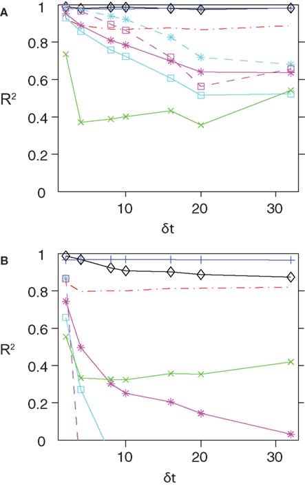
Figure 1. The quality of various approximations for different time bins and populations sizes. Here we plot the R2 values between the couplings obtained using various approximate methods and those found from Boltzmann learning versus δt (A) N = 40 and (B) N = 100. In both panel the colour code is as follows. Black, SM; Red, TAP; Blue, SM–TAP hybrid; Green, nMFT; Cyan, IP; Magenta low-rate limit of IP; Cyan with dashed line, IT; Magenta dashed lines, low rate limit of IT. For both population sizes and all time bins, the TAP, SM and hybrid approximations perform very well.
Extending the Independent-Pair Approximation
Extending the IP approximation is in principle straightforward. Instead of solving the problem of two isolated spins, we can solve the problem of three spins, i, j and k as shown in Section “Independent-triplet Approximation” in Appendix. This will lead to the IT approximation. In Figure 1
, we show the quality of the IT approximation for finding the couplings as compared to the Boltzmann solutions. For N = 40, we see that the IT approximation provides an improvement over IP for different values of δt. In Figure 1
, we also looked at the quality of the low rate limit of the IT approximation. In Section “Independent-triplet Approximation” in Appendix we show that, in the same way that the low rate limit of the IP approximation gives us the leading order terms of the low-rate expansion in Roudi et al. (2009a)
, the low rate limit of the IT approximation gives us the first order corrections to it. For N = 40, this is evident in the fact that the low-rate limit of IT outperforms the low-rate limit of IP for δt ≤ 15 ms. When the population size is large, however, IT and its low rate limit outperform IP for only very fine time bins. Even for δt = 4 ms, IP and IT and their low rate limits perform very bad.
One can of course build on the idea of the IP and IT approximations and consider n = 4, 5,…spins. However, for any large value of n, this will be impractical and computationally expensive, for the following reason. As described in Section “Independent-triplet Approximation” in Appendix for the case of the IT approximation, there are two steps in building an independent-n-spin approximation. The first one is to express the probability of each of the 2n possible states of a set of n spins in terms of the mean values and correlations of these spins. This requires inverting the 2n × 2n matrix. The second step, which is only present for n ≥ 3, is to express all correlation functions in terms of the mean values and pairwise correlations. Both of these steps become exponentially hard as n grows. Nonetheless, as shown in Section “Independent-triplet Approximation” in Appendix, even going to the triplet level can be a very useful exercise, as it offers a new way of computing the difference between the entropy of the true model and that of the independent model (Eq. 15a in Section “Entropy Difference”) as well as the difference between the entropy of the true model and that of the pairwise model (Eq. 15b in Section “Entropy Difference”). This derivation is considerably simpler than the original derivation of these equations based on the Sarmanov–Lancaster representation of the probability distribution described in Roudi et al. (2009a)
as well as the derivations in Section “The Partition Function, Entropy and Moments of a Gibbs Distribution in the Limit Nδ → 0” in Appendix, in which one starts by expanding the partition function of a Gibbs distribution. Furthermore, the IT approximation also yields a relation between the couplings and the mean values and pairwise correlations that coincides with leading term and the corrections found by low-rate expansion, as shown in Section “Independent-triplet Approximation” in Appendix.
Extending the Naive Mean-Field: Tap Equations
The nMF, IP and IT approximations are good for fitting the model parameters when the typical number of spikes generated by the whole population in a time bin is small compared to 1, i.e. when Nδ ≪ 1 (Roudi et al., 2009a
,b
), in which

For large and/or high firing rate populations, however, such approximations perform poorly for inferring the model parameters. It is possible to make simple corrections to the nMF approximation such that the resulting approximation performs well even for large populations. This is the so called TAP approximation (Thouless et al., 1977
). The idea dates back to Onsager, who added corrections to the nMF approximation, taking into account the effect of the magnetization of a spin i on itself via its influence on another spin j. Subsequently, it was shown that the resulting expression was exact for infinite-range spin-glass models (Thouless et al., 1977
). The TAP equations are

Differentiation with respect to mj then gives (i ≠ j)

One can solve Eq. 13 for the Jij and, after substituting the result in Eq. 12, solve Eq. 12 for the hi (Kappen and Rodriguez, 1998
; Tanaka, 1998
).
There are several ways to derive this expression for the pairwise distribution Eq. 2. In Section “Derivation of TAP Equations from Belief Propagation” in Appendix, we show that these equations can also be derived from the celebrated Belief Propagation algorithm used in combinatorial optimization theory (Mezard and Montanari, 2009
). When applied to spike trains from populations of up to 200 neurons, the inversion of TAP equations was shown to give remarkably accurate results (Roudi et al., 2009b
) for fitting the pairwise model. In Figure 2
, we show scatter plots comparing the couplings found by the TAP approximation versus the Boltzmann results for N = 100 and δt = 2, 10, 32 ms. The TAP approximations does well in all cases, and this is quantified in Figure 1
. In Figure 1
, we demonstrate the power of inverting the TAP equations for inferring the couplings for various time bins for both N = 40 and 100.
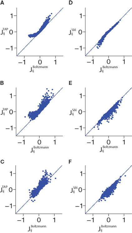
Figure 2. Scatter plots showing the results of TAP and SM approximations versus the Boltzmann results for various time bin sizes δt and N = 100. Panels (A–C) show the TAP results versus the Boltzmann results for data binned at 2, 10 and 32 ms, respectively. (D–F) show the same but for the SM approximation. Note that the structure of the error in estimating the couplings from the TAP equations changes when the size of the time bin is increased.
Sessak–Monasson Approximation
Most recently, Sessak and Monasson (2009)
developed a perturbative expansion expressing the fields and couplings of the Ising distribution as a series expansion in the pairwise correlation functions Cij. Some of the terms of the expression they found for the couplings could be summed up. It was noted in Roudi et al. (2009b)
, that one can think of the resulting expression as a combination of the nMF approximation and the IP approximation. The SM result can be written as
The reason why the last terms should be subtracted is discussed below.
Let us consider two neurons connected to each other. In the IP approximation we calculate the fields and couplings for this pair exactly within the assumption that they do not affect the rest of the network and vice versa. If we were to find the coupling between this pair of neurons using the nMF approximation Eq. 7, the result would just be the last term in Eq. 14. The reason why we should subtract it is now clear: the first term in Eq. 14 includes an nMF solution to the pair problem. We subtract this part and replace it by the exact solution of the pair problem. Figure 1
shows that this result is very robust to changing δt, although for N = 100, we can note a small decay in R2 with δt. The good performance of the SM approximation can be also seen in the scatter plots shown for N = 100 in Figure 2
. These observations support the SM approximation as a very powerful way of inferring the functional connections. Following the observation made in Roudi et al. (2009a)
, in Figure 1
, we also show how a simple averaging of the best approximate methods, i.e. TAP inversion and SM can provide a very accurate approximation to the couplings across different time bin and population sizes.
The experimental result that the binary pairwise models provide very good models for the statistics of spike trains is very intriguing. However, the message they carry about the architecture and function of the nervous system is not clear. This is largely due to the fact that, as reviewed in Section “Review of Experimental Results,” the experimental studies were conducted on populations of small number of neurons (N ∼ 10) and their implications on the real sized system are not trivial. Is it the case that observing a very good pairwise model on a subsystem of a large system constrains the structure and function of the real sized network? Does it mean that there is something unique about the role of pairwise interactions in the real sized system? Answering this question depends to a large extent on answering the extrapolation problem: to what degree the experimentally reported success of pairwise models holds for the real sized system? In what follows, we discuss some theoretical results that bear on this question.
Entropy Difference
The extrapolation problem was first addressed in Roudi et al. (2009a)
by analysing the dependence of the misfit measure δ (defined in Eq. 5) on N. The authors considered an arbitrary true distribution and computed the KL divergence between this distribution and an independent-neuron model as well as between it and the pairwise model. This was done using a perturbative expansion in Nδ ≪ 1, where δ is defined in Eq. 11. The results were the following equations:
where gind and gpair are constants that do not depend on N or δt and are defined in Eqs. 36a and 38a. Using these expressions for the KL divergences yields

Equations 15 and 16 show that for small Nδ, Δ will be very close to 0, independent of the structure of the true distribution. In other words, in this regime, a very good pairwise-model fit is a generic property and does not tell us anything new about the underlying structure of the true probability distribution. It is important to note that the perturbative expansion is always valid if δt is small enough. That is, simply by choosing a sufficiently small time bin, we can push Δ as close to 0 as we want.
In Roudi et al. (2009a)
, gpair and gind are related to the parameters of the pairwise model up to corrections of 𝒪(Nδ). In Section “The Partition Function, Entropy and Moments of a Gibbs Distribution in the Limit Nδ → 0” in Appendix, we present a different derivation by expanding the partition function of a true Gibbs probability distribution around the partition function of a distribution without couplings. In the following subsection, we also use the results of this derivation to compare the probability of synchronous spikes under the model and the true distributions. Furthermore, in Section “Independent-triplet Approximation” in Appendix, we extend the idea beyond the IP approximation and approximate the entropy of a given distribution as a sum over the entropies of triplets of isolated neurons. We show that this approach leads to Eq. 15 in a substantially simpler way than those reported in Roudi et al. (2009a) and Section “The Partition Function, Entropy and Moments of a Gibbs Distribution in the Limit Nδ → 0” in Appendix.
In Figure 3
, we show how DKL(p || pind), DKL(p || ppair) and Δ vary with N and δt for data generated from a simulated network. We have also plotted the predictions of the low-rate expansion Eqs. 15 and 16. As shown in these figures, the low-rate expansion nicely predicts the behaviour of the measurements from the simulations particularly for small N and δt. For δt = 10 ms, we have δ10 = 0.076 and for δt = 2 ms, we have δ2 = 0.019 (note that this gives δ10/δ2 = 3.95, a ratio that would have been equal to 5 if the bins were independent). Both the results from the low-rate expansion and those found directly from the simulations show that using finer time bins decrease Δ for fixed N.
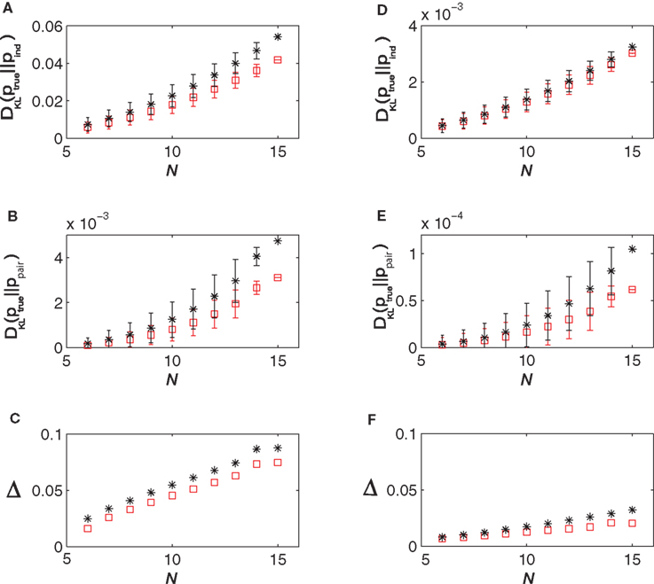
Figure 3. The quality of the pairwise and independent models for different time bins and populations sizes. (A) DKL(ptrue || Pind) versus N, (B) DKL(ptrue || ppair) versus N and (C) Δ versus N all for δt = 10 ms. (D–F) show the same things for δt = 2 ms. In all panels, the black stars represent quantities as computed directly from the simulated data, while the red squares show the predictions of the low-rate expansion, i.e. Eqs. 15 and 16. We have used 18000 s of simulated data for computing the plotted quantities and have corrected for finite sampling bias as described in Roudi et al. (2009b)
.
Probability of Simultaneous Spikes
As discussed in Section “Review of Experimental Results,” in addition to entropic measures such as KL divergence and Δ, which in a sense ask how well the model approximates the experimental probabilities of all possible spike patterns, we can restrict our quality measure to a subset of possible spike patterns. We can, for instance, ask how well the pairwise model approximates the probability of M simultaneous spikes. Similar to the case of Δ, before getting too impressed about the power of pairwise models in approximating the true distributions, we should find out what we expect in the case of an arbitrary, or random, true probability distribution.
Suppose now that we have a distribution over a set of variables of the form of Eqs. 27a and 27b. For this distribution, the probability that a set of M neurons, I = {i1,i2,…,iM} out of the whole population of N fire in a time bin while the rest do not is

Averaging over all possible I we get
where  are the mean values of the fields and pairwise, third-order etc coupling. In Section “The Partition Function, Entropy and Moments of a Gibbs Distribution in the Limit Nδ → 0” in Appendix, we show that, to leading order in Nδ, the external fields and pairwise couplings of fitted models (independent or pairwise) match those of the true model (see Eqs. 32a and 32b). Using this, we see that
are the mean values of the fields and pairwise, third-order etc coupling. In Section “The Partition Function, Entropy and Moments of a Gibbs Distribution in the Limit Nδ → 0” in Appendix, we show that, to leading order in Nδ, the external fields and pairwise couplings of fitted models (independent or pairwise) match those of the true model (see Eqs. 32a and 32b). Using this, we see that
To have well defined behaviour in large N limit, one should have  Eq. 19 show that, for M/N ≪ 1, both the independent and pairwise models are close to the true distribution. For M/N ∼ 𝒪(1) (of course still M/N < 1), the difference between the model and true probabilities of observing M synchronous spike increases. For all ranges of M, the difference is larger for the independent model. These predictions are consistent with the experimental results found in the retina (Tkacik et al., 2006
).
Eq. 19 show that, for M/N ≪ 1, both the independent and pairwise models are close to the true distribution. For M/N ∼ 𝒪(1) (of course still M/N < 1), the difference between the model and true probabilities of observing M synchronous spike increases. For all ranges of M, the difference is larger for the independent model. These predictions are consistent with the experimental results found in the retina (Tkacik et al., 2006
).In the above calculation, we compute the difference between the true and model values of q, i.e. the mean of the log probability of M synchronous spikes. However, one can also calculate the log mean probability of M synchronous spikes, i.e.
Calculating w is in theory very hard, because the second term above involves calculating the averages of exponential functions of variables. However, if the population is homogenous enough, such that the average couplings and fields from one sample of M neurons to the next does not change much, we can approximate the average of the exponential of a variable with the exponential of the average it. Doing this, will again lead to Eq. 19. The difference between the two measure w and q will most likely appear for small M where the averages of the fields and couplings depends on the sample of M neurons more strongly than when M is large.
In the previous sections, we described various approximate methods for fitting a pairwise model of the type of Eq. 2. We also studied how good a model it will be for spike trains, using analytical calculations and computer simulations. As we describe below, there are two issues with a model of the type of Eq. 2 that lead to new directions for extending the pairwise models studied here.
The first issue is the use of binary variables as a representation of the states of the system. For fine time bins and neural spike trains, the binary representation serves its purpose very well. However, in many other systems, a binary representation will be a naive simplification. Examples of such systems are modular models of the cortex in which the state of each cortical module is described by a variable taking a number of states usually much larger than 2. In Section “Extension to Non-binary Variables” we briefly describe a simple non-binary model useful for modelling the statistics of such systems.
The second issue is that by using Eq. 2 in cortical networks, one is essentially approximating the statistics of a highly non-equilibrium system with asymmetric physical interactions, e.g. a balanced cortical network, by an equilibrium distribution with symmetric interactions. This manifests itself in a lack of a simple relationship between the functional connectives to real physical connections. In our simulations we observed that there was no obvious relation between the synaptic connectivity and the inferred functional connections. Second, as we showed here and in our previous work, for large populations, the model quality decays. Although one can avoid this decay by decreasing δt as N grows, eventually one will get into the regime of very fine δt, where the assumption of independent bins used to build the model does not hold any more and one should start including the state transitions in the spike patterns (Roudi et al., 2009a
). In fact, Tang et al. (2008)
showed that even in the cases that the pairwise distribution of Eq. 2 is a good model for predicting the distribution of spike patterns, it will not be a good one for predicting the transition probabilities between them. These observations encourage one to go beyond an equilibrium distribution with symmetric weights. In the second extension, described in Section “Extension to Dynamics and Asymmetric Interactions,” we propose one such model, although a detailed study of the properties of such model is beyond the scope of this paper.
Extension to Non-Binary Variables
The binary representation is probably a good one for spike trains binned into fine time bins. However, for larger time bins where there is a considerable probability of observing more than one spike in a bin, as well as for a number of other systems, the binary representation may only serve as a naive simplification and going to non-binary representations is warranted. Example of such systems include the protein chains and modular cortical models. In probabilistic models of protein chains, each site is represented by a non-binary variable that takes one of its possible q states depending on the amino acid that sits on that site. In a number of models for the operations of cortical networks, one considers a network of interconnected modules, the state of each of which is represented by a non-binary variable (Kropff and Treves, 2005
; Russo et al., 2008
). Each state of one such variable corresponds to, e.g. one of the many memory states stored in the corresponding module.
For a set of non-binary variables σ = (σ1, σ2,…,σN), σi = 1,…,q, one can simply write down a maximum entropy pairwise Gibbs distribution as
where α and β go from 1,…,q and index the q possible states of each variable. For q = 2, the above distribution reduces to the binary case with Boolean variables, and when one forces  for α ≠ β one recovers the q-state Potts model. Similar to the binary case, here also one is given the experimentally observed values of
  and
and  and wants to infer the fields and couplings that are consistent with them.
for α ≠ β one recovers the q-state Potts model. Similar to the binary case, here also one is given the experimentally observed values of and and wants to infer the fields and couplings that are consistent with them.The approximate methods described in this paper can be adopted, with some effort, to the case of non-binary variable as well. In particular, it is easy to derive the difference between the entropy of the true distribution, the pairwise model and the independent model in the low-rate limit of the non-binary model. Assuming that  for α ≠ 1, the low-rate regime in the case of non-binary variables is characterised by N(q − 1)ε ≪ 1. In this regime, similar to the binary case, Spair − Strue ∝ [N(q − 1)ε]3 and Sind − Strue ∝ [N(q − 1)ε]2 and Δ = N(q − 1)ε, and consequently the pairwise model performs very well in the low-rate regime.
for α ≠ 1, the low-rate regime in the case of non-binary variables is characterised by N(q − 1)ε ≪ 1. In this regime, similar to the binary case, Spair − Strue ∝ [N(q − 1)ε]3 and Sind − Strue ∝ [N(q − 1)ε]2 and Δ = N(q − 1)ε, and consequently the pairwise model performs very well in the low-rate regime.As we described before, the low-rate regime is where most experimental studies on binary pairwise models were performed, and the result of the low-rate expansion of the entropies explains the reported success of binary pairwise models in those studies. On the other hand, the low-rate regime of the non-binary variable may be of little use. This is because the systems to which the non-binary representation should be applied are unlikely to fall into the low-rate regime. For instance, in the case of modular memory networks the low-rate regime would be the case in which the network spends a significantly larger time in its ground state (no memory retrieved) compared to the time it spends operating and retrieving memory. A more likely scenario is the one where all the states (memory or no-memory) have approximately similar probabilities of occurrence over a period of time. How useful pairwise models are in describing the statistics of such non-binary systems away from the trivial regime of the low-rate expansion is not known. Studying the quality of non-pairwise models in these cases and developing efficient ways to fit such models, in particular based on extensions of the powerful approximations such TAP and SM to non-binary variables will be the focus of future work. In particular, it is important to note that writing the SM approximation for the non-binary case will be a straightforward task in light of the relation we described between the SM, nMFT and IP approximations in Section “Sessak–Monasson Approximation.”
Extension to Dynamics and Asymmetric Interactions
The Glauber model (Glauber, 1963
) is the simplest dynamical model that has a stationary distribution equal to the Ising model distribution (Eq. 2). It is defined by a simple stochastic dynamics in which at each timestep δt = τ0/N one spin is chosen randomly and updated, taking the value +1 (i.e. the neuron spikes) with probability
Although the interactions Jij in the static Ising model are symmetric [any antisymmetric piece would cancel in computing the distribution (Eq. 2)], a Glauber model with asymmetric Jij is perfectly possible (Crisanti and Sompolinsky, 1988
; Ginzburg and Sompolinsky, 1994
).
This kinetic Ising model is closely related to another class of recently-studied network models called generalized linear models (GLMs, Okatan et al., 2005
; Truccolo et al., 2005
; Pillow et al., 2008
). In a GLM, neurons receive a net input from other neurons of the linear form,

and spike with a probability per unit time equal to a function f of this input. Maximum-likelihood techniques have been developed for solving the inverse problem for GLMs (finding the linear kernels that give the stimulus input and that from the other neurons in the network, given spike train data) (Okatan et al., 2005
; Truccolo et al., 2005
). They have been applied successfully to analysing spatiotemporal correlations in populations of retinal ganglion cells (Pillow et al., 2008
).
The Glauber model looks superficially like a GLM with instantaneous interactions and f(x) equal to a logistic sigmoid function 1/[1 + exp(−2x)]. But there is a difference in the dynamics: spins are not spikes. In the Glauber model, a spin/neuron retains its value (+1 or −1) until it is chosen again for updating. Since the updating is random, this persistence time is exponentially distributed with mean τ0. Thus a Glauber-model “spike” has a variable width, and the autocorrelation function of a free spin exhibits exponential decay with a time constant of τ0. In the GLM, in contrast, a spike is really a spike and the autocorrelation function (for constant input) is a delta-function at t = 0.
The time constant characterizing the kernel Jij(τ) in a GLM has a similar effect to τ0 in the Glauber model, but a GLM with an exponential kernel is not exactly equivalent to the Glauber model. In the GLM, the effect of a presynaptic spike is spread out and delayed in time by the kernel, but once it is felt, the postsynaptic firing rate changes immediately. In the Glauber model, the presynaptic “spike” is felt instantaneously and without delay, but the firing state of the neuron takes on the order of τ0 to change in response.
GLMs grew out of a class of single-neuron models called LNP models. The name LNP comes from the fact that there is a linear (L) filtering of the inputs, the result of which is fed to a nonlinear (N) function that specifies an instantaneous Poisson (P) firing rate. In the earlier studies, the focus was on the sensory periphery, where the input was an externally specified “stimulus”. An aim of this modelling effort was to improve on classical linear receptive field models. Thus, in the usual formulation of a GLM network, one writes the total input as a sum of two terms, one linear in the stimulus as in the LNP model and the other linear in the spike trains of the other neurons. Of course, one can trivially add a “stimulus” term in a Glauber model, so this differences is not an essential one.
Similarly, interactions with temporal kernels Jij(τ) can be included straightforwardly in a Glauber model. Such a model is equivalent to a GLM in the limit τ0 → 0. (One has to multiply the kernels by 1/τ while taking the limit, because the integrated strength of a “Glauber spike” is proportional to τ0, while that of an ordinary spike in a GLM is 1.)
One can derive a learning algorithm for a Glauber model, given its history, in a standard way, by maximizing the likelihood of the history. The update rule, which is exact in the same way that Boltzmann learning is for the symmetric model, is

where δsj(t) = sj(t) − 〈sj〉, the average is over the times ti at which unit i is updated, and bi = tanh−1〈si〉 = hi + ΣjJij〈sj〉.
One can also get a simple and potentially useful approximate algorithm which requires no iteration by expanding the tanh in Eq. 24 to first order in the Jij (i.e. to first order around the independent-neuron model). Then at convergence (δJij = 0) we have

which is a simple linear matrix equation that can be solved for the Jij.
The brain synthesizes higher-level concepts from multiple inputs received, and in many fields of research scientists are interested in inferring as simple a description as possible, given potentially vast amounts of data. Such processes of learning take a set of average values, correlations, or any other pattern in the data, and from these arrive at another representation, which is useful for speed or accuracy of prediction, for compressed storage of the data, as a grounds for decision making, or in any other aspect which improves the functionality or competitiveness of the brain or the researcher. Models and algorithms for learning in these contexts have been studied, in great detail, in neuroscience, image processing, and many other fields, for quite some time; consider, e.g. the introduction of Boltzmann machines more than a quarter of a century ago (Hinton and Sejnowski, 1983
), and the now more than 10-year-old monograph on learning in graphical models (Jordan, 1998
).
As one could have expected, there is a trade-off between the complexity of the model to be learned and the efficiency of the learning algorithms. Boltzmann machines are, in principle, able to learn very complex models, and provably so, but convergence is then quite slow; modern applications of those methods centre on various restricted Boltzmann machine models, which can be learned faster (Hinton, 2007
).
When we consider very large systems and/or problems where convergence time of the learning is a serious concern, then we are primarily interested fast learning processes. Often such fast processes come as approximation grounded on assumption on the model parameters, and the central issue is then obviously the accuracy of the learning outcomes based on those assumptions. In this paper we have revisited some classical and some more recent approximations of this kind that take their inspiration from statistical physics. The two simplest algorithms considered are nMF and IP approximation. As we have shown for neural data, both of these perform poorly except for small systems (small N), or for systems which have little variability (small value of Nδ), where δ here can be thought of as a proxy for the deviation from a uniform state. On the other hand, one generalization of each method, the TAP approximation for the nMF and the recent SM approximation for the IP approximation, perform much better. In the case of neural data analysed here, the parameter δ depends on the size of the time bin, δt. We showed that the TAP and SM approximations perform well for a large range of δt. In addition to studying the effect of δt on the performance of these approximations, we also studied the quality of pairwise models using a variety of methods. Using a few alternative analytical calculations, we derived mathematical expressions relating the quality of pairwise models to the size of the population and the lower order statistics of the spike trains. This analysis shows that for finer time bins the pairwise distribution becomes a better approximation to the true distribution of spike trains (Roudi et al., 2009a
). We confirmed this analytical result on synthetic data.
Our focus in this paper was on approximate inference methods that offer closed form equations relating model parameters to the measured statistics of the model. Another class include methods that rely on iterative algorithms. This class of approximate methods include the recent improvement of the Boltzmann learning in Broderick et al. (2007) and the “susceptibility propagation” (Mora, 2007
; Mezard and Mora, 2008
). These methods are generally slower than the closed form approximation, and a systematic comparison between their performance against what we have studied here is lacking.
To conclude, we have here framed the presentation in terms of inferring representations of neural data and assessing the goodness of the model. Although our focus was on neural data analysis, it is important to note that similar problems appear in many other fields of modern biology, for instance, e.g. in network reconstruction of gene regulatory networks, in genomic assembly in metagenomics projects, and in many other problems. Given the present explosion in sequencing technologies it is conceivable that the more novel applications will soon appear outside neuroscience.
The Partition Function, Entropy and Moments of a Gibbs Distribution in the Limit Nδ → 0
Suppose we have a true distribution of the following form

In this Appendix, we first find the relation between the external fields and pairwise and third order couplings. As we show below, this allows us to compute the probability of synchronous spikes. We also compute the entropy of this distribution, in the small spike probability regime to derive the expression in Eqs. 15. This task can be accomplished much more easily if we rewrite the distribution of Eq. 26 in terms of zero-one variables ri, instead of the spin variables si, i.e.
where the auxiliary inverse temperature β is introduced because it will allow us to compute the entropy, as will become clear later.
The crucial step in computing the relation between the moments, parameters and entropy of a distribution is computing its partition function. To compute the partition function of Eq. 27a, Z, we note that
where 〈〉0 indicates averaging with respect to the distribution

Note that p0 is not the independent model for p in Eqs. 27a and 27b but only the part of this distribution that includes the fields. In fact, as we show in the following (Eq. 32a) the fields of the independent model to p only match ℋi to 𝒪(Nδ) corrections, i.e.  When dealing with corrections to the fields and couplings, this note will be important.
When dealing with corrections to the fields and couplings, this note will be important.Since  a term with l distinct indices in the expansion of the term inside the average in Eq. 28 is of the order of δl. Therefore, to 𝒪((Nδ)3), we have
a term with l distinct indices in the expansion of the term inside the average in Eq. 28 is of the order of δl. Therefore, to 𝒪((Nδ)3), we have
where the sums over n, n1, n2, n3 and n4 run from 1 to infinity. Performing these sums yields
where ϕij = exp(β𝒥ij) − 1 and ϕijk = exp(β𝒦ijk) − 1. From Eq. 31, we can immediately compute the relation between the mean values, pairwise and three-point correlation functions and the parameters of the distribution. For β = 1, we have
The relations between mean values and pairwise correlations and the external fields and pairwise couplings in Eqs. 32a and 32b to their leading orders were reported previously in Roudi et al. (2009a)
, using a slightly different approach. However, the corrections and three-neuron correlations were not computed there.
An interesting result of this calculation is a relation between the three-neuron correlations for the pairwise distribution, i.e. when 𝒦ijk = 0, and the lower moments
The fact that, to leading order in Nδ, the external fields and couplings are determined by mean values and pairwise correlations allows us to compute the leading-order probabilities of synchronous spikes reported as we did in Section “Probability of Simultaneous Spikes.”
We can now use Eq. 31 to find the entropies of the distribution in Eq. 27a
From Eqs. 32a, 32b and 32c for an independent fit to the distribution Eq. 27a
Using the fact that  from Eq. 32a, and ϕij =
  from Eq. 32b, we get Eq. 15a with gind defined as
from Eq. 32a, and ϕij = from Eq. 32b, we get Eq. 15a with gind defined as
For a pairwise model to the distribution in Eq. 27a, we have  and thus
and thus
Using Eqs. 32c and 33, this will lead to Eq. 15a with gpair defined as
The Independent-Pair Approximation for the External Fields in the Limit δ → 0
Replacing δi = exp(ℋi)/[1 + exp(ℋi)] in Eq. 32a and solving to find ℋi we get
where in the second line we have used the fact that ϕij =  from Eq. 32b and that
  . Changing the variables from ri = 0,1 to the original spin variables si = ±1, we have
from Eq. 32b and that . Changing the variables from ri = 0,1 to the original spin variables si = ±1, we have
For the independent-pair (IP) approximation, on the other hand, we have
Summing  over j and subtracting the over counted terms from single spin contributions gives the same expression as Eq. 40. Therefore, the IP approximation to the external fields get the leading term and the first order corrections of the low-rate approximation correctly.
over j and subtracting the over counted terms from single spin contributions gives the same expression as Eq. 40. Therefore, the IP approximation to the external fields get the leading term and the first order corrections of the low-rate approximation correctly.Independent-Triplet Approximation
Considering the following Gibbs distribution over three Boolean variables ri, rj and rk,
we can use the definition of the mean values and correlations and write
Inverting the matrix of coefficients we can express the probabilities in terms of the mean values, pairwise and third order correlations. Using the result in
and similar equations for the other fields and couplings, we can also express these parameters in terms of mean values, pairwise and third order correlations. Before using Eqs. 48 and 49 as approximations for the parameters of a pairwise model, we need to perform two more steps.
The first step is a familiar one that we noted when dealing with the external fields in the IP approximation, namely the fact that  depends on j and k in addition to i and that
  depends on k. We can use the same logic that we used in building an IP approximation to the external fields, and build an approximation to the external fields that does not depend on j and k, and an approximation to the couplings that does not depend on k. For example, for the case of the pairwise couplings we get
depends on j and k in addition to i and that depends on k. We can use the same logic that we used in building an IP approximation to the external fields, and build an approximation to the external fields that does not depend on j and k, and an approximation to the couplings that does not depend on k. For example, for the case of the pairwise couplings we get
The second step has to do with the fact that Eqs. 44a and 44b (as well as their transformed version after performing the first step, e.g. Eq. 45) depend on the third order correlations in addition to the pairwise correlations and the mean values. Hence to derive an expression that relates model parameters to pairwise correlations and mean values we should first find the third order correlation in terms of them. Note that this step is not present in the IP approximation. To express the third order correlations in terms of the lower order statistics we take advantage of the following equation
Writing the probabilities in terms of the moments, this equation can be solved to find the third order correlations in terms of the mean values and pairwise correlations. The equations have two imaginary solutions for  which are unphysical, and one real solution, which is the correct solution to be considered. The resulting expression for
  in terms of the mean values and pairwise correlations is complicated. However, in the limit of
  it can be shown to have the same form as the one reported in Eq. 33. We noted in the text that in this limit, the IP approximations to the couplings will give the same result as the leading order term of Eq. 32b for the couplings. With the independent-triplet (IT) approximation, we can go one step further, and as can be shown by doing a small amount of algebra, we can recover 𝒪(Nδ) corrections to the couplings in that we calculated in Eq. 32b.
which are unphysical, and one real solution, which is the correct solution to be considered. The resulting expression for in terms of the mean values and pairwise correlations is complicated. However, in the limit of it can be shown to have the same form as the one reported in Eq. 33. We noted in the text that in this limit, the IP approximations to the couplings will give the same result as the leading order term of Eq. 32b for the couplings. With the independent-triplet (IT) approximation, we can go one step further, and as can be shown by doing a small amount of algebra, we can recover 𝒪(Nδ) corrections to the couplings in that we calculated in Eq. 32b.As mentioned in Section “Extending the Independent-pair Approximation,” one can continue the above process to build approximations based on quadruples of spins and so on. However, this soon becomes difficult in practice for the reason that solving equations of the type Eq. 46 to find the higher moments in terms of the mean values and pairwise correlations will be as difficult as the original problem of finding the external fields and couplings of the original N body problem in terms of the mean values and correlations. Nevertheless, this simple triplet expansion offers an alternative derivation of Eq. 15, simpler than the derivations in Roudi et al. (2009a) and Section “The Partition Function, Entropy and Moments of a Gibbs Distribution in the Limit Nδ → 0” in Appendix. Here we show this for Eq. 15b, as deriving Eq. 15a will be similar but less involved. To derive Eq. 15b using the triplet expansion, we approximate the entropy of the whole system of N neurons as a sum of the entropies of all triplets denoted by Sijk. We then expand the resulting expression keeping terms of up to 𝒪(δ3) noting that  The result takes the form of
The result takes the form of
where Q(x) = x log(x). For a pairwise model, the IT approximation to the entropy in the limit  has the same form, except that
  of the true model should be replaced by
  (see Eq. 33), i.e.
has the same form, except that of the true model should be replaced by (see Eq. 33), i.e.
Using Eqs. 32c, 47 and 48 yields Eq. 15b.
Derivation of Tap Equations from Belief Propagation
In this appendix we derive the TAP equations (Eq. 12) starting from the Belief Propagation update rules. Let us begin with the result to be established. The TAP equations are a set of nonlinear equations for the magnetizations mi, which we will write:

Here hi is the external field acting on spin i, εJij are the pairwise couplings, and the notation J ∈ ∂i means that the sum is over neurons j connected with neuron i. As we also did in the text in Eq. 12, the above equation is generally quoted with ε set to one and without the error term of cubic order in ε.
Starting from the pairwise distribution (Eq. 2), we define the following distribution, with the auxiliary variable ε that we set to 1 in the end of our calculation

and the exact marginal distribution over spin si is defined by

where the sum goes over all spins except si. The exact magnetization of spin si is then
Belief Propagation is a family of methods for approximately computing the marginal distributions of probability distributions (Kschischang et al., 2001
; Yedidia et al., 2003
; Mezard and Montanari, 2009
). Since the model defined by Eq. 50 contains only pairwise interactions, it is convenient to adopt the pairwise Markovian random field formalism of Yedidia, Freeman and Weiss (Yedidia et al., 2003
). Note that the important recent contribution by Mezard and Mora uses a more general formalism, which may prove to be more convenient in the perspective of extending an “inverse BP” learning algorithm beyond pairwise models (Mora, 2007
).
Belief Propagation applied to the model in Eq. 50 in the Yedidia–Weiss–Freeman formalism is built on probability distributions, called BP messages, associated with every directed link in the graph. If i → j is such a link, starting at i and ending at j, then the BP message ηi→j(sj) is a probability distribution on the variable sj associated to node where the link ends. For Ising spins one can use the parametrization

where mi→j is a real number called the cavity magnetization. BP is characterized by two equations, the Belief Propagation update equations, and the Belief Propagation output equations. The BP update equations are used0 iteratively to find a fixed point, which is an extremum of the Bethe free energy. At the fixed point, the BP update equations form a (large) set of compatibility conditions for the η’s which, for the model Eq. 50, read

The BP output equations determine the marginal probability distributions from the η’s and read
where Ωj→i and Ωi in Eqs. 54 and 55 are normalizations. To lighten the notation, we will not distinguish between the exact marginals, as in Eq. 51, and the approximate marginals from BP, as in Eq. 55.
We now write the BP update and BP output equations using the cavity magnetizations, mi→j, from Eq. 53. The notation simplifies if one define an ancillary quantity

in terms of which the BP update equation can be written as

and the BP output equation as

The task is now to expand the right hand side of Eq. 58 in ε and compare with the TAP equations, Eqs. 49. To do this, we first note that

This follows from expanding Eq. 57 in ε, using the result in Eq. 56, and finally, expanding the logarithm. We then rewrite the BP output Eq. 58 as

Since mj = tanh(hj + Σk∈∂j qk→j) (no expansion in ε) we want to separate qi→j and hi + Σk∈∂j qk→j in the arguments of the tanh’es in Eq. 60, and according to Eq. 59, qi→j is of order ε. This means that we can write, to order ε,
Introducing this into Eq. 60, we finally have

which was to be proved.
The authors declare that the research was conducted in the absence of any commercial or financial relationships that could be construed as a potential conflict of interest.
Mora, T. (2007). G’eométrie et inférence dans l’optimisation et en théorie de l’information. Ph.D. thesis, Université Paris Sud - Paris XI. http://tel.archives-ouvertes.fr/tel-00175221/en/
Tang, A., Jackson, D., Hobbs, J., Chen, W., Smith, J. L., Patel, H., Prieto, A., Petrusca, D., Grivich, M. I., Sher, A., Hottowy, P., Dabrowski, W., Litke, A. M., and Beggs, J. M. (2008). A maximum entropy model applied to spatial and temporal correlations from cortical networks in vitro. J. Neurosci. 28, 505–518.