1
Institute for Theoretical Computer Science, Graz University of Technology, Graz, Austria
2
Software Competence Center Hagenberg, Hagenberg, Austria
The Parallel Circuit SIMulator (PCSIM) is a software package for simulation of neural circuits. It is primarily designed for distributed simulation of large scale networks of spiking point neurons. Although its computational core is written in C++, PCSIM’s primary interface is implemented in the Python programming language, which is a powerful programming environment and allows the user to easily integrate the neural circuit simulator with data analysis and visualization tools to manage the full neural modeling life cycle. The main focus of this paper is to describe PCSIM’s full integration into Python and the benefits thereof. In particular we will investigate how the automatically generated bidirectional interface and PCSIM’s object-oriented modular framework enable the user to adopt a hybrid modeling approach: using and extending PCSIM’s functionality either employing pure Python or C++ and thus combining the advantages of both worlds. Furthermore, we describe several supplementary PCSIM packages written in pure Python and tailored towards setting up and analyzing neural simulations.
Given the complex nonlinear nature of the dynamics of biological neural systems, many of their properties can be investigated only through computer simulations. The need of researchers to increase their productivity while implementing increasingly complex models without each time having to reinvent the wheel has become a driving force to develop simulators for neural systems that incorporate best known practices in simulation algorithms and technologies, and make it accessible to the user through a high-level user-friendly interface (Brette et al., 2007
). It has also been brought to attention that it is of importance to use large neural networks with biologically realistic connectivity (on the order of 104 synapses per neuron) as simulation models of mammalian cortical networks (Morrison et al., 2005
). Simulation of such large models can practically be done only by exploiting the computing power and the memory of multiple computers by means of a distributed simulation.
There are different neural simulation environments presently available and although many of them were initially envisioned for a specific purpose and domain of applicability, during continuing development their set of features expanded to improve generality and support construction of a wide range of different neural models; see Brette et al. (2007)
for a recent overview. The two most prominent tools are NEURON (Carnevale and Hines, 2006
; Hines and Carnevale, 1997
) and GENESIS (Bower and Beeman, 1998
) which aim at simulation of detailed multi-compartmental neuron models and small networks of detailed neurons. Another class of quite general neural simulation environments which focus on the simulation of large-scale cortical network models and the improvement of their simulation efficiency through distributed computing include NEST (Gewaltig and Diesmann, 2007
; Plesser et al., 2007
), NCS (Brette et al., 2007
) and SPLIT (Hammarlund and Ekeberg. 1998
). There are also more dedicated neural simulation tools like iNVT (iLab Neuromorphic Vision Toolkit)
1
which is an example of a package specifically tailored for the domain of brain-inspired neuromorphic vision. All of the above simulation environments support parallel simulation of one model on multiple processing nodes by using commodity clusters and many of them can also be run on super-computers. The simulation tool PCSIM described in this paper is designed for simulating neural circuits with a support for distributed simulation of large scale neural networks. Its development started as an effort to redesign the previous CSIM simulator
2
(Natschläger et al., 2003
) and augment its capabilities, with the major extension being the implementation of a distributed simulation engine in C++ and a new convenient programming interface. The aim was to provide a general extensible framework for simulation of hybrid neural models that include both spiking and analog neural network components together with other abstract processing elements while making the setup and control of parallel simulations as convenient as possible for the user. Hence, given its current set of features, the PCSIM simulator is closest to the second group (NEST, NCS, SPLIT) of neural simulation environments mentioned above.
Performing a neural network simulation usually requires combined usage of several additional software tools together with the simulator, for stimulus preparation, analysis of output data and visualization. Being able to steer all the necessary tools from one programming environment reduces the complexity of setting up simulation experiments since all development can be done in a single programming language and the burden of developing utilities for conversion of data formats between heterogeneous tools is avoided. Given its object-oriented capabilities and its strong support for integration with other programming languages, the Python programming language is a very promising candidate for providing such a unifying software environment for simultaneous use of various scientific software libraries. As Python is becoming increasingly popular in the scientific community as an interpreting language of choice for scientific applications, the developers of many neural simulator tools decided to provide a Python interface for their simulator in addition to its legacy interface in a custom scripting language. Moreover, a simulation tool called Brian which uses Python as an implementation language was recently developed to bring to the user the full flexibility of an interpreting language in specifying and manipulating neural models (Goodman and Brette, 2008
).
In spite of the evident practical advantages in using Python as the single programming language for all tasks during a neural modeling life cycle, there is the apparent discrepancy between the need for computational performance of the simulation and construction of the model on one hand, and rapid development of the model on the other. Using C++ can solve the performance issue, but will decrease the productivity of the modeler and requires higher level of programming skills and experience. In contrast Python is easy to learn, flexible to use and significantly increases the productivity of the modeler, however it lags far behind C++ in performance
3
. Hence, instead of adopting a single language, an alternative is to enable an easy mix and match of both languages during the development of a model, i.e. to introduce a hybrid modeling approach (Abrahams and Grosse-Kunstleve, 2003
).
In this paper we will describe how the modular object-oriented framework of PCSIM in combination with an automated interface generation supports such a hybrid modeling approach.
In particular, we briefly review PCSIM’s main features (see Overview) before we describe the automated process to generate the Python interface (see Python Interface Generation). In the Section “Network Construction” we detail PCSIM’s network construction application programming interface (API), which is a central part of PCSIM’s object-oriented modular framework. In the Section “Custom Network Elements” we demonstrate another advantage of the hybrid modeling approach: we show how PCSIM’s concept of a general network element can be used as an interface to another simulation tool. While these examples concentrate on the Python aspect of the hybrid modeling, we show in the Section “Extending PCSIM Using C++” how the user can easily extend PCSIM’s functionality using C++. Additional PCSIM packages implemented in Python are reviewed in the Section “PCSIM Add-Ons Implemented in Python”. In the Section “Discussion” we discuss and summarize the presented concepts and approaches.
We would like to note that it is outside the scope of this article to describe the algorithmic aspects of PCSIM’s computational C++ core (this will be reported elsewhere) and all the details of the full object-oriented modular framework.
Architecture
The high-level architecture of PCSIM is depicted in Figure 1
. The PCSIM library written in C++ (
libpcsim) constitutes the core of the simulator. The API of the PCSIM library is exposed to the Python programming language by means of the Python extension module pypcsim (see Python Interface Generation for details). The library is made up of three main components: the simulation engine with its communication system, a pool of built-in network elements (i.e. neuron and synapse types) and the network construction layer. Before presenting the network construction layer in detail in the Section “Network Construction” we will briefly describe in the next paragraphs the main features of the underlying simulation engine and its communication system.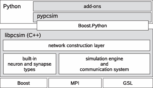
Figure 1. Architecture overview of PCSIM.
The simulation engine integrates all the network elements (typically neurons and synapses) and advances the simulation to the next time step, and uses its communication system to handle the routing and delivery of discrete and analog messages (i.e. spikes and e.g. firing rates or membrane voltages) between the connected network elements. PCSIM’s simulation engine is capable of running distributed simulations where the individual network elements are located at different computing nodes. Setting up a distributed simulation is handled easily from a users point of view: there are no (or very little) code changes necessary when switching from a non-distributed to a distributed simulation. The distributed simulation mode is intended for employing a cluster of machines for simulation of one large network where each machine integrates the equations of a subset of neurons and synapses in the network. A distributed PCSIM simulation runs as an MPI
4
based application composed of multiple MPI processes located on different machines
5
. The implementation of the spike routing, transfer and delivery algorithm between the nodes in a distributed simulation is based on the ideas presented in Morrison et al. (2005)
. In addition PCSIM offers the possibility to run a simulation as a multi-threaded application, both in a non-distributed and a distributed setup. The multi-threaded mode is intended for performing simulations on one multi-processor machine when one wants to split the computational workload among multiple threads in one process, each running on a different processor. However, we should note that the multi-threaded simulation engine is still undergoing optimization, as we are working on improvement of the scaling of the multi-threaded simulation to match the scaling achieved with an equivalent distributed simulation.
Scalability and Domain of Applicability
One of the goals of the development of PCSIM was enabling simulations of large neural networks on standard computer clusters through distributed computing. By utilizing the parallel capabilities of PCSIM the simulation time for a model can be reduced by using more processors (on multiple machines) as computing resources.
As a test of the scalability, we performed multiple simulations with the PCSIM implementation of the CUBA model described in Brette et al. (2007)
, with different number of leaky integrate-and-fire neurons (4000, 20000, 50000 and 100000) and distributed over a different number of processors (each processor on a different machine). We changed the resting potential in the neuron equations from −49 to −60 mV such that the network does not show any spontaneous activity. In order to elicit a spiking activity in the network, an input neuron population of 1000 neurons was connected randomly to it with probability 0.1, i.e. each neuron in the network receives inputs from on average 100 input neurons. The input neurons fired homogeneous Poisson spike trains at a rate of 5 Hz. The simulation was performed for 1 s biological time with a time step of 0.1 ms. We have set the connection probability within the network to 0.1, in order to reach realistic number of 10000 synapses per neuron for the network size of 100000 neurons. The transmission delay of spikes was set to 1 ms. We scaled the weights of the network so that the mean firing rate of the neurons was between 2.4 and 2.7 Hz for all network sizes (more precisely 2.68, 2.55, 2.52 and 2.45 Hz for the network with 4000, 20000, 50000 and 10000 neurons, respectively).
The used machines had Intel® Xeon™64 bit CPUs with 2.66 GHz and 4 MB level-2 processor cache, and 8 GB of RAM. They were connected in a 1 Gbit/s Ethernet LAN.
If we assume ideal linear speed-up, then the expected simulation time of a model on N machines given the actual simulation time on K machines is equal to the simulation time on K machines times K divided by N. In the evaluation of the scaling, for the estimation of the expected simulation time (see Figure 2
) we used the measured simulation time of the model on the minimum number of machines used for that particular network size. Namely, we used the actual simulation time on K = 1 machine for the network sizes of 4000 and 20000 neurons, and the simulation time on K = 4 and K = 16 machines for the network sizes of 50000 and 100000 neurons respectively.
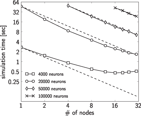
Figure 2. Simulation times of the CUBA network distributed over different number of processing nodes, compared to the expected simulation time (dashed line) (see text for details). Four different sizes of networks were simulated: 4000 neurons with on average 1.6 × 10⁶ synapses (squares), 20000 neurons with on average 40 × 106 synapses (circles), 50000 neurons with on average 250 × 106 synapses (diamonds) and 100000 neurons with on average 1 × 10⁹ synapses (crosses). The plotted simulation times are averages over 12 simulation runs. The variation of simulation time between different simulation runs was small, therefore we did not show it.
Figure 2
shows that in the case of 4000 neurons the computational load on each node is quite low, hence the cost of the spike message passing dominates the simulation time which results in sub-linear scaling. For the networks with 20000 and 50000 neurons the actual simulation time is shorter than the expected simulation time indicating a supra-linear speed-up for up to 24 nodes. For more than 24 nodes the actual simulation time approaches the expected simulation time. The reason for the supra-linear speed-up is more efficient usage of the processor cache when the network is distributed over larger number of nodes (Morrison et al., 2005
). For the network with 100000 neurons the speed-up is not distinguishable from the expected linear speed-up (taking K = 16 nodes as the base measurement).
The combination of features that PCSIM supports makes it suitable for various types of neural models. Its domain of applicability can be considered across two complementary aspects: the size of networks that can be simulated, and the variety of different models that can be constructed and simulated, determined by the available neuron and synapse models, plasticity mechanisms, construction algorithms and similar. Concerning the size of models, because of its distributed capabilities PCSIM is mainly targeted towards large neural systems with realistic cortical connectivity composed of 105 neurons and above. As the results from the scalability test show, a spiking network with 105 neurons and 104 synapses per neuron can be simulated in a reasonable time on a commodity cluster with about 20 machines, and the speed-up is linear when more machines are employed for the simulation. Regarding the support for construction of various different models in PCSIM, the generality of the communication system and the extensibility with custom network elements enables simulation of hybrid models (spiking and analog networks) incorporating different levels of abstraction. By utilizing the construction framework also structured models with diversity of neuron and synapse types and varying parameter values can be defined and simulated, and the built-in support for synaptic plasticity further expands the domain of usability towards models that investigate synaptic plasticity mechanisms.
In order to enable a hybrid modeling approach we wanted to use a Python interface generation tool that was capable of wrapping PCSIM’s object-oriented and modular API such that the Python API will be as close as possible to the C++ API. Our choice for this purpose was the Boost.Python
6
library (Abrahams and Grosse-Kunstleve, 2003
). The strength of Boost.Python is that by using advanced C++ compile-time introspection and template meta-programming techniques it provides comprehensive mappings between C++ and Python constructs and idioms. There is support, amongst others, for exception handling, iterators, operator overloading, standard template library (STL) containers and Python collections, smart pointers and virtual functions that can be overridden in Python. The later feature makes the interface bidirectional, meaning that in addition to the possibility of calling C++ code from Python, user extension classes implemented in Python can be called from within the C++ framework. This is an enabler for the targeted hybrid modeling approach; we will see examples for this later on in this article.
However, using Boost.Python without any additional tools does not lead to a solution where the interface can be generated in an automatic fashion since for each new class added to the library’s API one would have to write a substantial piece of Boost.Python code. As automatic Python wrapping of the C++ interface is one of the main prerequisites for leveraging a hybrid modeling approach, a solution is needed to automatically synchronize the Python and C++ API of a library like
libpcsim. Fortunately, there exists the Py++ package
7
which was developed to alleviate the repetitive process of writing and maintaining Boost.Python code. Py++ by itself is an object-oriented framework for creating custom Boost.Python code generators for an application library written in C++. It builds on GCC-XML
8
, a C++ parser based on the GCC compiler that outputs an XML representation of the C++ code. Py++ uses this structured information together with some user input, in form of a Python program, and produces the necessary Boost.Python code, constituting the Python interface for a specified set of C++ classes and functions (see Figure 3
).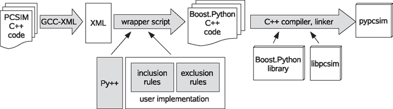
Figure 3. The processing steps in the generation of the Python interface for PCSIM.
Finally the Boost.Python C++ code is compiled and linked together with the C++ library under consideration (
libpcsim in our case) to produce the Python extension module containing the Python API of the library (pypcsim in our case). Thus, the work of the developer (and the user as we will see later on) reduces to a definition of high-level rules to select which classes and methods should be exposed.For the generation of the PCSIM Python interface
pypcsim, we split the rules Py++ needs into two subsets, inclusion and exclusion rules (see Figure 3
). The inclusion rules contain the rules that mark a selected set of classes to be exposed to Python. The exclusion rules contain the post-processing, where some of the methods of the classes that were included in the inclusion rules are marked to be excluded, and call policies are defined for the included methods that require them
9
. Py++ allows to specify the rules in a high-level, generic fashion, making them robust to changes in the interface of the PCSIM C++ library. Hence, in most cases changes in the PCSIM API did not require changes in the Python program that generates the wrapper code, which simplified its maintenance. An example of such a high-level rule would be “In all classes that are derived from class A, do not expose the method that returns a pointer of type B”. Such a general rule will then be still valid if for example we introduce more classes derived from A, or add additional functions that return a pointer of type B in some of the classes.To summarize, the Python integration of PCSIM using Boost.Python together with the Py++ code generator allowed us to come up with a solution to automatically expose PCSIM’s object-oriented and modular API bidirectionally in Python. In the following sections we will show how such an bidirectional integration of PCSIM into Python can practically be used and which possibilities and advantages arise.
A large portion of the Python PCSIM interface is devoted to the construction of neural circuits. At the lowest level PCSIM provides methods to create individual network elements (i.e. neurons and synapses) and to connect them together.
On top of these primitives a powerful and extensible framework for circuit construction based on probabilistic rules is built. The source of inspiration for the interface of the framework was the Circuit Tool in the CSIM simulator
10
and PyNN, an API for simulator-independent procedural definition of spiking neural networks (Davison et al., 2008
). We will use a concrete example
11
, described in more depth in the next subsection, to present the network construction framework and its typical use cases where emphasis is put on those features that were enabled by the bidirectional Python interface generated by the approach described in the Section “Python Interface Generation”.
The Example Model
We selected the model to be simple enough for didactic reasons, but complete enough with all the elements necessary to explain the main novel concepts of the interface and its Python extensibility features. The connectivity patterns are based on experimental data that we use in our current research work. The model consists of a spatial population of neurons located on a 3D grid with integer coordinates within a volume of 20 × 20 × 6. 80% of the neurons in the model are excitatory, and the rest are inhibitory. The excitatory neurons are modeled as regular spiking and the inhibitory neurons as fast spiking Izhikevich neurons (Izhikevich, 2004
). The connections between excitatory neurons in the network are created according to the trivariate probabilistic model defined in Buzas et al. (2006)
. This connectivity model describes the distribution of the excitatory patchy long-range lateral connections found in the superficial layers of the primary visual cortex in cats that depends on the lateral distance of the cells and their orientation preference. Orientation preference is the affinity of V1 cells to fire more when a bar with a specific orientation angle is present in their receptive fields. The connectivity rule is defined by the following equations that express the connectivity probability between two excitatory cells.
li = (xi, yi) and lj = (xj, yj) are the 2D locations and ϕi and ϕj are the orientation preferences of the pre- and post-synaptic neurons i and j. The function G introduces the dependence of the connectivity probability on the lateral distance between the neurons, and V models the dependency on the differences in the orientation preferences of the neurons. C, κ and σ are scaling coefficients. The values for the preferred orientation angles of the neurons in the example are generated by evolving a self-organizing map (SOM) (Obermayer and Blasdel, 1993
). Additionally the conduction delay of a connection between excitatory neurons is probabilistically dependent on the distance between the 3D locations of its pre- and post-synaptic neurons.

Here N(μ, σ, bl, bu) is a bounded normal distribution representing the transmission velocity of the axon. The li = (xi, yi, zi) and lj = (xj, yj, zj) denote the 3D locations of the pre- and post-synaptic neurons i and j. A random value from N(μ, σ, bl, bu) is sampled as follows: first a random number from a normal distribution with mean μ and standard deviation σ is drawn and if that value is not within the range [bl, bu], then another value is drawn from an uniform distribution with that range. D0 represents a proper scaling factor in the formula.
The Framework: Object-Oriented, Modular and Extensible
Figure 4
shows the basic concepts of PCSIM’s construction framework together with their interactions during the construction process. This framework allows model specification in terms of populations of neurons connected by probabilistically defined connectivity patterns called projections.
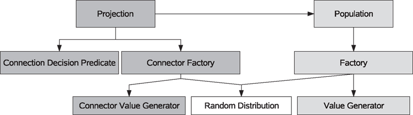
Figure 4. A diagram of the most important concepts within the network construction interface. The arrows indicate a “uses” relationship between the concepts.
A population of network elements utilizes several object factories to generate the network elements. A factory encapsulates the logic for the neuron and synapse generation decoupled from the other parts of the construction process. Every time a new neuron is to be created in a population the factory is used to generate the neuron object. The object factories can use either random distribution objects or value generators to generate values for the parameters and attributes of the network element instances. When we talk about a parameter we mean a parameter of the differential equations used to model a neuron or synapse. In contrast an attribute describes any other (more abstract) property of a network element. In our example the orientation preference ϕ will be such an attribute of an excitatory neuron.
A projection manages connections between two populations. During the construction phase of a projection a connection decision predicate is used to determine whether a connection should be created for a pair of neurons. A connector factory is then used to create instances of the connector elements like synapses (this is analogous to the object factory for populations). The connector factory also uses random distributions or connector value generators for the parameter values of the connector elements. In order to implement a specific construction algorithm, the user typically just needs to implement custom value generator and connection decision predicate classes, as we will demonstrate in the following subsections.
Factories: Creating Network Elements from Models
We will start constructing the network model by defining the classes (or families) of neuron models: inhibitory and excitatory neurons. This is accomplished by defining an element factory for each family. As explained in the definition of “The Example Model” the excitatory neurons have an orientation preference ϕ which depends on the location of the neuron in the population. For this reason we will associate the attribute
phi with each excitatory neuron:
The statement above creates a factory for the excitatory family of neurons based on a regular spiking (RS) Izhikevich neuron model (Izhikevich, 2004
) where
IzhiNeuron is a built-in network element class. The keyword argument Vinit = UniformDistribution(…) associates a uniform random number generator with the initial membrane voltage Vinit. This has the effect that whenever the factory is used to generate an actual instance of an excitatory neuron, the parameter Vinit will be randomly chosen from the interval [−50, −60] mV. Finally the keyword argument attribs = dict( phi = … ) has two effects: a) the attribute phi is attached to exc_factory and b) the custom value generator OrientationPreferValGen is used to generate a particular value for phi each time exc_factory is asked to generate an instance of an excitatory model neuron. The value of the phi attribute will be used afterwards for the creation of synaptic connections.In the example we implement the custom value generator
OrientationPreferValGen in pure Python. This is enabled by the particular feature of Boost.Python which allows C++ virtual functions to be overridden from within Python.
Value generators (in this case to be derived from
PyAttributePopObjectValueGenerator) have a simple interface composed of the constructor --init-- and the method generate which have to be implemented by the user. In our particular example we create the orientation map, that maps 2D coordinates to an orientation preference angle in the constructor, and will use it in the method generate. The map is based on the SOM algorithm encapsulated in the Python class OrientationMapSOM (details not relevant here). The generate method is called to determine the value of the orientation angle attribute phi whenever a neuron instance from the factory has to be created. The value generator inherits several convenient methods from its base class that one can use for accessing properties of the neuron for which generate is called, like self.loc to get the 3D location of the neuron within a population (see next section). We then pass the x and y coordinates to the orientation map (method pref) in order to calculate the value of the orientation preference angle.For the inhibitory neuron model we create a similar factory:
The difference to the excitatory neuron model is that a fast spiking (FS) Izhikevich neuron model is used and the attribute dictionary
attribs = dict( ) is empty. This is because there is no orientation preference of the inhibitory cells in the considered model.Neuron Populations
A population in PCSIM represents an organized set of neurons that can be manipulated as one structural unit in the model. In the
AugmentedSpatialPopulation that we will use in this example, the neurons have associated 3D coordinates, a family identifier, and an extensible set of custom attributes that the user can attach to each of the neurons. We already encountered this in the previous section. The family identifier allows the definition of multiple families/classes of neurons, i.e. subsets of neurons with similar properties, within a single population. Our population will have two families of neurons, the family of excitatory and the family of inhibitory neurons. For each of the two families of neurons we have specified in the previous section a factory that will be used to generate the neuron instances within the population.
Note that the first argument (
net) specifies the overall network to which this population of neurons will belong. The class CuboidIntegerGrid3D, which is a built-in specialization of the more general concept of an arbitrary set of points in 3D, defines the possible locations for the neurons (integer coordinates within a volume of 20 × 20 × 6). The population is to be composed of two families of neurons (excitatory and inhibitory), created by the two given factories (exc_factory and inh_factory). To accomplish this we use a RatioBasedFamilies object which randomly chooses for each 3D location from which family of neurons the particular instance will be created. Specifying the ratio 4:1 for excitatory to inhibitory neurons yields the desired 80% excitatory neurons. The class RatioBasedFamilies is a built-in specialization of the general concept of a spatial family identifier generator which encapsulates the logic for deciding which factory to use depending on the 3D location.For the purpose of more convenient setup of connections later on, the created population is split into two sub-populations, one for each family.
Projections: Managing Synaptic Connections
The synaptic connections in the network construction interface are created by means of projections. A projection is a construct that represents a set of synaptic connections originating from one population of neurons and terminating at another population
12
. PCSIM has built-in construction algorithms for creating various types of connection projections, like constant probability random connectivity or random connectivity with probability dependent on the distance (or lateral distance) between the neurons.
However, to create a projection with a specific connectivity pattern, one usually defines a custom connection decision predicate. A decision predicate decides for an individual pair of neurons whether to form a connection based on the parameters and attributes of those neurons. In our example we implemented the connection decision predicate
OrientationSpecificConnPredicate in pure Python, encapsulating the probabilistic rule for connection making from Eq. 1, which states that the connection probability depends on the distance between, and the orientation preferences of the pre- and post-synaptic neurons.
The
PyAugmentedConnectionDecisionPredicate base class is used when one has to define a custom connection decision predicate that uses the neuron attributes and connects neurons from populations of type AugmentedSpatialPopulation. To complete the implementation of the predicate, it is required to override the decide method and fill the constructor with the necessary initializations. The method decide is called within the connection construction process for each candidate pair of neurons that could be connected and is expected to output true (make a connection) or false (no connection). In our example, we create an instance (orient_conn_prob) of the OrientationSpecConnProbability class to calculate the probability according to the Eq. 1 (the full implementation of the class is available in the Supplementary Material). This instance is called in the decide method with the orientation preferences of the candidate source and destination neurons and their lateral distance as arguments. The orientation preferences are obtained via the src_attr and dest_attr methods (inherited from the base class), and the lateral distance via the dist_2d method. By comparing a uniformly distributed random number to the calculated probability a Bernoulli distribution with the desired probability for the outcome true is generated.Before we can create the projection we have to define a connector factory (class
ConnFactory) that will be used to generate the synapse objects within the projection.
The connector factory differs from the element factory objects used in conjunction with neuron populations, in that the parameters of the created objects (typically synapses) can depend on the attributes of the source and destination network elements they are connecting. In our example, the connector factory for the connections between excitatory neurons is based on a current-based synapse model with exponentially decaying post-synaptic response (class
StaticSpikingSynapse in PCSIM). Additionally, the DelayCond value generator is associated to the delay parameter of the synapse, which produces distance dependent delay values according to Eq. 4. The DelayCond is a built-in value generator in PCSIM.Now we can create the projection that will generate all recurrent connections between the excitatory neurons.
We specify in the constructor of the projection the connectorfactory for generation of the synapses and the
PredicateBasedConnections class instance that iterates over all candidate pre- and post-synaptic neurons and delegates the decision whether to make a connection to the connection decision predicate OrientationSpecificConnPredicate given as an argument.A connection decision predicate is typically used when in the probabilistic connectivity definition the probability that two neurons are connected depends on the attributes and parameters of the two neurons and is independent from the other created connections. In the general case, with such a connectivity, a separate decision whether to make a connection has to be made at each candidate neuron pair, yielding a complexity of the wiring algorithm that is quadratic with respect to the number of neurons. In a distributed scenario, a speed-up of the construction is possible by splitting the wiring workload among the multiple machines the model is simulated on. If the number of machines is increased with the number of neurons, keeping the number of neurons per node fixed, and if we assume that the number of input synapses per neuron does not increase, then the wiring time will scale linearly with the number of neurons.
For other connectivity schemes where further optimizations are possible, a faster wiring algorithm can be implemented directly in the class that iterates over the neuron pairs. For example, for the case of constant probability random connections, a special
RandomConnections class that implements faster wiring can be used instead of PredicateBasedConnections. When using the RandomConnections, the wiring time is proportional to the number of created connections if the network is constructed on a single machine, and remains constant in the distributed case with the assumption that the number of machines is increased proportionally with the number of neurons
13
.The PCSIM communication system is general in a sense that it supports spiking and analog messages as communication between network elements. The network elements are not restricted to one type of message and can have multiple input and output ports, each of them capable of either receiving or sending spiking or analog messages (see Figures 5
A,B).

Figure 5. (A) Network elements of different type (with different arrangement of input and output ports) interconnected together in a PCSIM network. Different colors of ports, gray or white, mark their different types, spiking or analog. (B) Neurons and synapses are specific subtypes of the more general concept of an network element. (C) Schematic diagram of the embedding of a network simulated with the Brian simulator into a PCSIM network element.
The generality of the framework allows the user to implement custom processing elements that map multiple inputs to multiple outputs and plug them in a network model inter-connected together with spiking or analog neural networks. Such custom network elements can either be implemented in C++ (see Extending PCSIM Using C++) or in pure Python. This feature of PCSIM has various potential uses. For example the user can implement new neuron types for a preliminary experiment in Python first, instead of directly implementing them in C++. Another possible usage is to implement more abstract or complex elements like a whole population of spiking neurons in Python by using vectors from the numerical Python package
numpy
14
(Oliphant, 2007
) for step-by-step integration of the equations. This approach has been shown to have good performance, and is applicable for homogeneous neuron populations, where all neuron instances have the same neuron model (Brian simulator, Goodman and Brette, 2008
).We detail such an example in this section, where the Brian simulator is used to implement a population of spiking neurons as a single network element, and then plug it into a PCSIM simulation together with other built-in network elements.
The spiking neural network model we will simulate with Brian is the modified version of the CUBA benchmark model described in the Section “Overview”, with a network size of 4000 neurons. We have used the same connectivity probability of 0.02 and the same weights as in Brette et al. (2007)
, instead of the modified 0.1 connectivity probability and scaled weights in the Section “Overview”. The PCSIM network element that we will create to encapsulate the Brain network has 1000 spiking input ports and 4000 spiking output ports (see Figure 5
C). Each of the output ports is associated to one neuron.
To implement this model as a PCSIM network element, one has to implement a Python class
BrianCircuit derived from PySimObject. In the constructor of this class the Brian spiking network is created and initialized.
The mapping of the PCSIM input ports to a Brian neuron group is managed by the simple auxiliary neuron group named
PCSIMInputNeuronGroup (see the Supplementary Material for the implementation). The reset method resets the state of the network to time step t = 0, which is achieved by calling the reinit method of the Brian network, and initializing the membrane potential vector P.V to random values from an uniform distribution.
The step-by-step iteration of the network is done in the overridden
advance method which performs one time-step update of the Brian network with the update method and the tick method of the associated Brian clock object. At the end of each time step the generated spikes of the population are gathered and delivered to the output ports of the PCSIM network element.
Note that no Python loops are present, the
setOutputSpikes method that transfers the spikes is implemented in C++ in the base class PySimObject, so there is no performance loss caused by the transfer of spikes from Brian to PCSIM and vice versa.The new
BrianCircuit network element class can then be instantiated and added to a PCSIM simulation. The following code segment creates an instance of the Brian spiking network, adds it as a network element, sets up the input and runs the simulation for 2.0 s [1000 neurons that emit Poisson spike trains at rate 5 Hz (PoissonInputNeuron) are connected to the 1000 input ports of the Brian network element]
15
.
The object-oriented framework of PCSIM can be extended by the user at many different levels. Typical extensions of PCSIM include either implementations of new neuron and synapse types, or implementations of classes encapsulating custom construction rules in the network construction interface, as we have illustrated in the previous sections. By utilizing the features of the Boost.Python library and Py++, the extensions can be implemented either in pure Python as already shown or in C++.
For creating C++ extensions, PCSIM provides a tool that compiles the custom C++ classes, automatically generates the Python wrapper interface for these and packs everything into a separate Python extension module. In order to simplify the procedure of creating a custom extension, the user starts the implementation from an extension template contained in the PCSIM distribution. Let us assume that we want to implement two classes: a new neuron type
MyNeuron and a new synapse type MySynapse. Once the C++ implementation is finished, there are three additional steps that have to be done to produce the PCSIM extension module.First, the C++ source files of the extension have to be enlisted in the file
module_recipe.cmake. This file is read by PCSIM’s C++ build tool CMake
16
.
As the second step, we have to specify the names of the classes we want to include in the Python interface in the file
python_interface_specification.py which holds the extension module interface specification. For our example the inserted lines should look like:
Note that the argument
M in the code above denotes the Py++ representation of the C++ code of the custom PCSIM extension to be built, with its rather intuitive query interface.The name of the extension module (in our example
my_pcsim_module) is specified in both module_recipe.cmake and python_interface_specification.py files. Finally, the compilation is done using the special purpose command-line compilation tool for PCSIM extensions:
The compiled extension module then can be imported and used within Python as any other module.
The main
pypcsim module should always be imported before any PCSIM extension modules, because the classes in the extension are derived from classes in pypcsim and these classes should be already in the Python namespace. The user can develop multiple PCSIM extension modules that can be used simultaneously in one simulation.The creation of a PCSIM extension as a separate Python extension module relies on the support of Boost.Python and Py++ for component-based development, so that C++ types from one Python extension module can be passed to functions from another extension module while still preserving the information about the cross-module C++ inheritance relationships. This enables object instances from the classes in the extension module to be used within the PCSIM object-oriented framework in the main
pypcsim module. The component-based development has also the advantage that during the development of new custom classes only the extension module has to be recompiled, not the whole pypcsim library.During the compilation of the PCSIM extension module the same processing steps happen as for the main
pypcsim module (see Figure 3
). We use the same scripts both for generation of the Python interface of the main PCSIM package and for the Python integration of PCSIM extension modules. Since the post-processing exclusion rules are expressed with the Py++ query interface in a generic way, they are applicable also to the wrapping of the extension classes. This is due to the fact that extension classes are derived from base classes in the PCSIM object-oriented framework and as such share their common properties on which the rules are based. Hence, the interaction of the user with the interface generation and the module compilation reduces to specifying a list of the C++ source files, and a list of classes to be exposed in Python. The rest of the process is automatized and the details are hidden behind the command-line interface of the special compilation tool for PCSIM extensions.On top of the main PCSIM Python API (encapsulated in
pypcsim) several additional packages have been developed. They are implemented in pure Python and heavily rely on many third party scientific Python packages. The purpose of these packages is either to augment the capabilities of PCSIM, or add additional separate functionalities that are suitable to be used together with PCSIM.PyNN.PCSIM
The objective of the PCSIM development to adopt ongoing initiatives to define standards for model specification of neural networks that would foster interoperability between different simulators is reflected in the support of the PyNN project
17
(Davison et al., 2008
). The PyNN project is an effort to create a standardized, unified Python-based API for procedural specification of neural network models aiming at easier exchange of models between simulators. The user interface of PCSIM has been augmented with an additional software layer to support the PyNN API making it possible to use models specified in PyNN within PCSIM. Due to the fact that PyNN was one of the sources for inspiration of the PCSIM interface, the concepts between the two interfaces match closely, so the translation of the PyNN statements in corresponding PCSIM statements was straightforward and did not require substantial programming logic that could have hindered the performance of the interface. The
pyNN.pcsim package is an integral part of the PyNN distribution.pypcsimplus
After we started to use PCSIM for our simulation purposes, it was becoming apparent that adding another layer above the interface of the
pypcsim module can greatly simplify the routine tasks that are usually performed while setting up and running simulations. The pypcsimplus package was created with the intention to fill this gap. Note that the pypcsimplus package is dependent on PCSIM. For a more comprehensive, simulator independent tool-set for neural simulations, we refer the reader to the NeuroTools package
18
. In the following paragraphs we will describe two main components of the pypcsimplus package and give a demonstration of its use
19
.Recordings
In PCSIM the value of a parameter or output port is recorded during a simulation by connecting it to a proper recording network element. The purpose of the
Recordings class is to provide simpler means to set up recorders and saving the recorded data during a PCSIM simulation. For example it allows to create a population of recorders that record the activity of a population of elements with each recorder connected to one of the elements (e.g. the spiking output of a population of neurons). For example
schedules the recording of all spikes in the population
nrn_popul, the membrane potential Vm of a single neuron (my_nrn), and the weights of a group of plastic synapses. To save that data to an HDF5 file
20
one would use the command
At any time later on, the saved data can be loaded from the file in a new
Recordings object.
The members and attributes of the newly created
Recordings object r are numpy arrays or Python lists holding the recorded data. For example r.Vm and r.W will be numpy arrays with the recorded values of the membrane potential of the neuron and with the evolution of the recorded synaptic weights during the simulation, respectively. Note that if the user switches to a distributed simulation the same code, without any changes, can be used.To summarize, the
Recordings class simplifies the specification, storage and retrieval of recorded data by• providing automatic detection of the type of the recorded data based on the recorder classes, and conversion of the recorded data to appropriate HDF5 data structures.
• implementing automatic gathering and sorting of recorded data from all processing nodes in a distributed simulation, and saving it in HDF5 in the same format as if the simulation was executed on a single node.
These functionalities are hidden behind a convenient user interface and are manipulated in the same manner in both single-node and distributed simulation modes. For the implementation of the
Recordings class, the mpi4py
21
(Dalcín et al., 2008
) and pytables
22
packages were used.Experiment-model framework
Simulation, modeling and development environments in various fields (e.g. electronic circuit design, software engineering, signal processing, mechanical engineering) usually include a library of already developed reusable components that are readily available to the modeler. In the area of computational neuroscience, there is a similar effort to provide resources for easier reusability of models, e.g. online databases of already published models (Hines et al., 2004
), or constructs within the simulator that allow encapsulation of a simpler model as a well-defined component that can be used as a building block at a higher-level of abstraction. As a first step towards a component-based modeling with PCSIM, we have set up a light-weight framework that could leverage and encourage encapsulation of some generic parts of a model as reusable components, which can be exchanged among modelers.
The basis of the framework is composed of three classes:
Model, Experiment and Parameters. The Model is a base class which the user inherits from when he wants to develop a model component. Several model components can be combined together to create a new model component. The Experiment class provides means to perform a controlled simulation with an already developed custom Model class. It encapsulates different facilities regarding saving output data to files, configuration of models, saving the current version of the scripts, naming of different runs of experiments etc. The configuration of the models is done with a Parameters class holding the model parameters in a hierarchical structure. For creating instances of the Experiment and Model classes remotely within the IPython parallel computing framework
23
(Pérez and Granger, 2007
) there are RemoteExperiment and RemoteModel proxy classes, which can be used to manipulate remote experiment and model instances in the same way as if they were local.Pypcsimplus in action
We will demonstrate in the following paragraphs how pypcsimplus, together with other general scientific and computational neuroscience Python packages, can be utilized to perform an analysis of the activity of the Brian spiking network example from the Section “Custom Network Elements”. In particular we will investigate what effect a change in the injected input in the network will have on the cross-correlogram of its spike response.
At the beginning we will set up the recording of the spiking output of all 4000 neurons in the network. After creating a
Recordings object, we create a population of recorders to record the spikes from the 4000 output ports of the BrianCircuit network element.
We have accomplished this by using the
record_ports function from the pypcsimplus package, used to specify recording of a set of output ports. After the simulation is performed, the recordings are saved in a HDF5 file for subsequent retrieval.In another script we setup the analysis of the output data and the plotting. After the creation of the
Recordings object by loading the recorded data from the saved HDF5 file, we plot the spiking activity of the network for the first 0.4 s of the simulation with the plot_raster function in pypcsimplus (see Figure 6
A).
Figure 6. Plots from the output analysis example with the
pypcsimplus package. (A) Spike response of the spiking network implemented in the Section “Custom Network Elements”, with input neurons emitting spikes generated from a homogeneous Poisson process with a rate of 5 Hz, for the first 0.4 s of the simulation. (B) Cross-correlogram of the spike response of the network model from (A). (C) Spike response of the spiking network implemented in the Section “Custom Network Elements”, when the input neurons emit spikes generated from an inhomogeneous Poisson process with a rate changing according to a sinusoidal function (see text for details). (D) Cross-correlogram of the spike response of the network model from (C).
plot_raster uses the plotting routines from the matplotlib
24
package (Hunter, 2007
) to realize the plotting.Additionally we will calculate and plot the cross-correlogram of the spiking activity, defined as the histogram of time differences between the spike times from two different spike trains, calculated and summed over a set of randomly chosen pairs of neurons from the network. To achieve this, we utilize the
pypcsimplus function avg_cross_correlate_spikes.
In our case the cross-correlogram is calculated from the spike times of 2000 randomly chosen pairs of neurons from the network, for time lags within the range [−200 ms, 200 ms] and a bin size of 1 ms. We then plot the cross-correlogram values with the
bar function from matplotlib (the plot is shown in Figure 6
B)
25
.In the example in the Section “Custom Network Elements”, the input neurons were setup to generate a homogeneous Poisson spike trains with 5 Hz rate. Now we will modify the input generation so that the input neurons will emit inhomogeneous Poisson spike trains, with a firing rate r(t) = 5(1 + sin(2π 10t)). First we create a population of input neurons of type
SpikingInputNeuron that emit an explicitly given sequence of spike times.
Then we iterate through all the input neurons and set the spike sequence of each input neuron according to the previously defined inhomogeneous Poisson process. For the generation of the inhomogeneous Poisson spike time sequences we invoke the
inh_poisson_generator method of an instance of the StGen (stimulus generator) class available in the NeuroTools Python package for computational neuroscience. The method accepts three parameters, a sequence specifying the time moments where the rate changes (parameter t), the sequence of the new firing rate values at these time moments (parameter rate) and the duration of the spiking process (parameter t_stop)
26
.
The spike raster and the cross-correlogram obtained after rerunning the simulation with the newly defined input are shown in Figures 6
C,D, respectively.
Through this demo we have elucidated to the reader how a typical PCSIM simulation run is performed in Python, and the benefits that come from the utilization of Python as a unifying scripting environment within which PCSIM is used together with its add-on
pypcsimplus and other scientific and computational neuroscience Python packages. Additionally to their side-by-side usage with PCSIM, the Python scientific packages are harnessed also in the bundling of common recipes and reoccurring usage patterns in the PCSIM extra add-on packages, as in the case of pypcsimplus. The collection of Python scientific packages presently available cover a broad enough range of functionalities to enable, in almost all cases, handling all of the steps of a modeling effort in Python (e.g. stimulus preparation, response analysis and plotting as shown in the demo). The data communication between the different packages and PCSIM typically reduces to passing Python sequences (lists or numpy arrays) from one package to another.pylsm
The pylsm package is aimed to support the analysis of the computational properties of cortical microcircuits within the liquid state machine (LSM) approach (Maass et al., 2002
). In this approach multiple simulation trials are performed where input spike trains, drawn from a defined input distribution, are injected in the cortical circuit, and a readout which reads the spiking activity of the circuit is trained by a supervised learning algorithm to approximate some function of these inputs.
The framework contains all the necessary machinery for performing the simulations and the training of the readout
27
. In a typical task the user defines the neural circuit to be used as a liquid, chooses the desired input distribution, the input-output mapping function, and the learning algorithm for the readout from the ones available in the package, and then performs the LSM training and testing procedures. For example, the user can define a distribution of inputs which consist of different time segments, and each of these time segments contains a jittered version of some predefined spike train template. In the available learning algorithms for the readout a least-square algorithm with non-negative constraints is also included. It can be used to train a linear readout with the biologically more realistic constraint that all the weights originating from excitatory (inhibitory) neurons are positive (negative) (Haeusler and Maass, 2007
).
The application programming interface of PCSIM is an object-oriented framework composed of many classes interacting together to achieve the desired operation. Within this framework we introduced several novel concepts like element and connector factories, value generators and connection decision predicates. The user can customize and extend this framework by deriving from the interface classes of the API to implement his own specific network elements or network construction algorithms.
The Wrapping Approach
There exist several possible approaches for implementing a Python interface of a simulation software library implemented in C/C++. An extension to the NCS software called Brainlab (Drewes, 2005
) uses generation of a file from Python with declarative specification of the model which is then loaded in the simulator. Another common method is to use interpreter-to-interpreter interaction with the conversion of data structures between Python and C++ handled by means of the Python/C API, an approach adopted by NEURON (Hines et al., 2009
) and NEST (Eppler et al., 2008
). This method is applicable only if the simulator already has an interpreting interface. For the creation of PyMoose (Ray and Bhalla, 2008
), the Python interface of MOOSE
28
, the developers applied the interface generator tool SWIG
29
(Beazley, 2003
). Certainly, one can also implement a Python interface by using solely the Python/C API.
Since PCSIM’s Python interface was to be newly developed, only the later two options were applicable. We opted for the interface generator tool approach combined with automatic wrapper code generation, since from the available options it seemed to us the fastest way, in terms of the amount of development effort required, to achieve the desired Python wrapping of the PCSIM object-oriented framework. One of our goals for the integration of PCSIM with Python was to simplify and support a hybrid modeling approach by enabling the user to implement extensions of the PCSIM object-oriented framework in Python and/or C++, while not having to bother with details regarding the interoperability between these two programming languages.
The excellent support of Boost.Python for advanced C++ concepts and appropriate mapping of corresponding idioms between the two languages allowed us to expose the complete PCSIM API, currently ≈300 classes, to Python in a non-intrusive way. This means that the fact that the PCSIM API is to be exposed to Python does not impose any changes at the C++ level nor does it put any constraints on its design. Furthermore the compilation of the
libpcsim library itself does not depend on any Python library or wrapping code.Bidirectional Interface and Hybrid Model Definition
One of the features of Boost.Python enabling the hybrid approach is the ability to derive Python classes from the wrapped interface classes, and override the virtual functions. Hence, such custom Python class methods can be called from within C++ and thus allow an integration of Python code into the PCSIM C++ code. A similar bidirectional interface has been implemented between Python and NEURON (Hines et al., 2009
), where Python can issue commands towards NEURON, but also Python code can be called and executed from within NEURON in an active Hoc session
30
. In PCSIM the two-way interaction between Python and C++ enables user customizations to be coded in pure Python, and then plugged into the PCSIM C++ framework. This brings additional flexibility and freedom to the user, meaning that he can first do fast implementations in Python, e.g. extensions to the network construction interface (see Network Construction), in the prototyping phase, and afterwards the implementation can be ported to C++ to gain maximum performance.
The ability to define PCSIM network elements in Python opens a possibility for a seamless Python-C++ integration also during the simulation, not only in the network construction stage. The example described in the Section “Custom Network Elements” shows that network elements can be implemented in Python, by using vectorized techniques employing the highly efficient numerical Python package
numpy (which is implemented in C). This adds flexibility, since the equations describing the element can be changed quickly without any necessary compilation while not sacrificing performance, since by using numpy vectors, the integration algorithm is broken down in elementary vector operations thus avoiding any loops within Python that could be detrimental for the performance.This approach seems also to be advantageous when one wants to implement network elements that have some abstract processing logic, e.g. signal processing filters, machine learning algorithms or similar. In this case one can utilize a large set of available C++ libraries that have Python bindings, for an efficient implementation, and handle in Python the transfer of data from the input ports of the network element to the input methods of the library, and from the output of the library to the output ports of the network element.
The possibility to implement PCSIM network elements in pure Python offers a convenient way to achieve run-time interoperability between PCSIM and other neural network simulators (Cannon et al., 2007
), provided that the simulator has a Python interface, allows control of the simulation process at individual time steps, and has the possibility to write input and read output data during the simulation at each time step. As shown in the example in the Section “Custom Network Elements”, we have successfully implemented interoperability with the Brian simulator, which possesses the aforementioned capabilities. One interesting further application of this interoperability could be a distributed simulation of a large neural network where the sub-networks on each node are implemented with the Brian simulator, and the parallel communication is handled by PCSIM’s communication system. Another possible approach of using Python as a glue language to achieve simulator interoperability is to setup a Python script as a top-level coordinator of a step-by-step simultaneous execution of two simulators, where the necessary data transfer between the simulators is realized through intermediate Python data structures (Ray and Bhalla, 2008
).
High-Level Wrapping Specification and Extensibility
Since the interface of PCSIM has a fine granular structure, composed of many decoupled classes (≈300) this implies that there are many classes to be wrapped and exposed to Python. It would simply be impossible to manually manage all the necessary Boost.Python wrapper code. Furthermore, the possibility of adding extensions to the interface puts additional constraints to the wrapping approach to be robust enough to work for the extension classes too, without any significant intervention from the user. Nevertheless, by exploiting the powerful interface generator tool Py++ the wrapping of such a large number of classes is rendered feasible
31
. We were able to specify high-level generic rules within Py++ for the definition of the wrapping of all the classes in the PCSIM API and their sensible extensions. To be precise, the Python program that specifies the rules for the Python interface generation for ≈300 classes is about 400 lines of Python code. As these rules apply for the extensions too, the user can easily extend the PCSIM simulator with its own custom C++ classes and compile them in a separate Python extension package, which can be used together with the main
pypcsim package (the tool support for this is included in PCSIM). This was made possible by the Boost.Python and Py++ support for cross-module inheritance relationships and component-based development (see “Extending PCSIM Using C++”).To summarize, by the easy extensibility of its interface both in Python and C++, PCSIM enables the modelers to think hybrid when developing their models (Abrahams and Grosse-Kunstleve, 2003
).
Python as a Scripting Environment
Providing a Python interface to a neural simulator increases its versatility and consequently the productivity of the modelers in many ways. The object oriented design of the language, its expressive and clean syntax, allows the modeler to focus on the high-level logic of the model instead of struggling with the intricacies and the nuts and bolts of the programming language. Furthermore, there is a growing number of general scientific and specific computational neuroscience software tools available as Python packages, for numerical calculations, scientific functions, plotting, saving data to files, parallel computing etc. We have used several scientific Python packages to enhance PCSIM with useful utilities on top of its basic interface. As we have illustrated through a simple example in the Section “PCSIM Add-Ons Implemented in Python”, in combination with such Python packages PCSIM can be used as the main component of a Python-based neural simulation environment where all steps within a neural model development life-cycle, from the specification of the model and performing the simulations, to storage of simulation output data, data analysis and visualization can be performed. Overall, the integration of PCSIM with Python added additional valuable facilities to the user, turning PCSIM into a full-fledged neural simulation environment.
PCSIM Resources
Many resources for PCSIM can be found at its web page
32
. The web page contains a user manual, examples, installation instructions, complete class reference documentation and the complete material for the tutorial that was given at the FIAS Theoretical Neuroscience and Complex Systems summer school held in Frankfurt, Germany in August, 2008. The users can discuss topics and pose questions concerning usage and installation of PCSIM on the pcsim-users mailing list on Sourceforge®
33
where the PCSIM development project is hosted. In the future, the user manual will continuously undergo extensions and revisions to better organize the content and to include additional topics and more elaborate information about the PCSIM concepts and constructs. Additional examples covering various PCSIM features will also be made available on the web site.
The authors declare that the research was conducted in the absence of any commercial or financial relationships that could be construed as a potential conflict of interest.
We would like to thank Eilif Muller and Andrew P. Davison for helpful discussions, and the two reviewers for providing valuable suggestions that helped improving the manuscript. Written under partial support of the Austrian Science Fund FWF, project #S9102-N04, as well as project #FP6-015879 (FACETS, http://facets.kip.uni-heidelberg.de
) and #216593 (SECO, http://www.seco-project.eu
) of the European Union.
- ^ http://ilab.usc.edu/toolkit/home.shtml
- ^ http://www.lsm.tugraz.at/csim
- ^
The simulation tool Brian mentioned above, heavily uses the numerical Python package
numpy(Oliphant, 2007 ) written in C to achieve reasonable performance. - ^ http://www-unix.mcs.anl.gov/mpi/
- ^ To be precise, we use the C++ bindings offered by the MPICH2 library, where currently none of the advanced features of the MPI-2 standard are used.
- ^ http://www.boost.org/doc/libs/release/libs/python/doc/
- ^ http://www.language-binding.net/
- ^ http://www.gccxml.org
- ^ Call policies define the change of ownership of objects that cross the boundaries of the C++ library, i.e. the object passed from Python to the C++ library and from the C++ library to Python.
- ^ http://www.lsm.tugraz.at/circuits
- ^ The full source code of this example is available in the Supplementary Material.
- ^ The source and destination populations can be the same if the goal is to create recurrent connections in one population.
- ^ It is out of scope of this article to detail the algorithms behind the efficient implementation of the network construction framework in the distributed simulation scenario; this will be reported elsewhere.
- ^ http://numpy.scipy.org
- ^
The
net.connect(src_id, src_port, dest_id, dest_port)method connects the port numbersrc_portof the element with idsrc_id, to the port numberdest_portof the element with iddest_id. - ^ http://www.cmake.org
- ^ http://neuralensemble.org/trac/PyNN
- ^ http://neuralensemble.org/trac/NeuroTools
- ^ There are other miscellaneous utilities present within the pypcsimplus package, as for example tools for easier management of IPython parallel computing cluster instances, routines for inspection of the structure of an already created networks in PCSIM and routines for processing and analysis of spike train data.
- ^ http://www.hdfgroup.org/HDF5/
- ^ http://mpi4py.scipy.org
- ^ http://www.pytables.org/moin
- ^ http://ipython.scipy.org
- ^ http://matplotlib.sourceforge.net
- ^ For clarity reasons, we only give the main matplotlib plotting command in the example code blocks, and omit the additional formatting commands used for Figure 6 .
- ^ Time in neurotoools is specified in milliseconds, hence the division by 1000 when we need to convert the spike time sequence in seconds before inserting it in a PCSIM neuron.
- ^ It has similar features as the package described in Natschläger et al. (2003) , which was implemented in Matlab and was part of the CSIM package.
- ^ http://moose.sourceforge.net/
- ^ http://www.swig.org
- ^ Hoc is the native NEURON interpreting language.
- ^ The only drawback we encounter is the rather long compile time when recompiling the whole Python interface. This is due to the fact that Boost.Python heavily uses C++ templates.
- ^ http://www.igi.tugraz.at/pcsim
- ^ http://www.sourceforge.net/projects/pcsim
Brette, R., Rudolph, M., Carnevale, T., Hines, M., Beeman, D., Bower, J. M., Diesmann, M., Morrison, A., Goodman, P. H., Harris, F. C., Jr., Zirpe, M., Natschläger, T., Pecevski, D., Ermentrout, B., Djurfeldt, M., Lansner, A., Rochel, O., Vieville, T., Muller, E., Davison, A. P., Boustani, S. E., and Destexhe, A. (2007). Simulation of networks of spiking neurons: a review of tools and strategies. J. Comput. Neurosci. 23, 349–398.