1
Department of Psychiatry, Harvard Medical School, Charlestown, MA, USA
2
Neural Systems Group, Massachusetts General Hospital, Charlestown, MA, USA
There has been substantial recent growth in the use of non-invasive optical brain imaging in studies of human brain function in health and disease. Near-infrared neuroimaging (NIN) is one of the most promising of these techniques and, although NIN hardware continues to evolve at a rapid pace, software tools supporting optical data acquisition, image processing, statistical modeling, and visualization remain less refined. Python, a modular and computationally efficient development language, can support functional neuroimaging studies of diverse design and implementation. In particular, Python’s easily readable syntax and modular architecture allow swift prototyping followed by efficient transition to stable production systems. As an introduction to our ongoing efforts to develop Python software tools for structural and functional neuroimaging, we discuss: (i) the role of non-invasive diffuse optical imaging in measuring brain function, (ii) the key computational requirements to support NIN experiments, (iii) our collection of software tools to support NIN, called NinPy, and (iv) future extensions of these tools that will allow integration of optical with other structural and functional neuroimaging data sources. Source code for the software discussed here will be made available at http://www.nmr.mgh.harvard.edu/Neural_SystemsGroup/software.html
.
The efficient conduct of neuroimaging experiments requires a diverse and complex assortment of computational resources. It follows naturally that constructing complete systems for data acquisition, analysis and display would be facilitated by the use of highly versatile, modular development environments. Functional neuroimaging data collection requires accurate timing of both stimulus displays and user responses, with near real-time graphics and device polling capabilities. The structural and functional neuroimaging datasets acquired over the course of a typical 1- to 2-h experimental session can exceed 10 gigabytes in size. These high data collection rates, along with the need to monitor the data flow for quality assurance purposes, require excellent system throughput and real-time data display capabilities to support experimental monitoring. Once acquired, neuroimaging datasets must undergo substantial preprocessing, data reduction and statistical processing to accurately model the many, often hierarchical, sources of variance in the raw data. These sources can include instrument noise, temporal autocorrelation, head motion, cardiovascular physiological effects, within-subject task effects, within-group effects, and between-group treatment effects. Finally, the statistical results must be displayed in an intuitive and easily comprehensible form using publication quality graphics.
While the construction of tools for each of these steps poses a substantial challenge, many current Python modules provide an excellent foundation on which to build data acquisition and processing pipelines. These advantages are already evident in magnetic resonance imaging (MRI) and electroencephalography (EEG) data processing applications, as demonstrated by other papers this issue. However, near-infrared neuroimaging (NIN) is one domain for which no Python tools exist, and for which only two non-commercial software solutions are available (Huppert, 2006
; Ye et al., 2009
). We have therefore been developing a suite of Python modules to support the computational aspects of NIN data acquisition, analysis, and display. While our particular collection of tools is specialized for handling NIN data, the general design principles have broader application in experimental and theoretical neuroscience. We plan to release sub-modules under a BSD license, posting them at http://www.nmr.mgh.harvard.edu/Neural_SystemsGroup/software.html
as they reach beta level stability.
We begin with an explanation of the physical and biological basis for NIN, followed by a brief comparative review of its chief uses. To provide context for our software development efforts, “Computational Requirements and Software” begins by describing the logistical and computational requirements associated with NIN experiments. The remainder of that section then describes the individual acquisition, analysis and visualization modules comprising the NinPy package, followed by a discussion of future software development directions in “Future Extensions”.
Principles of Near-Infrared Neuroimaging
The physical principles underlying NIN are relatively simple, and similar to those encountered in pulse oximetry. The human scalp and skull are sufficiently transparent to the near-infrared (NIR) light wavelengths between 650 and 950 nm to enable non-invasive optical monitoring of physiological modulations associated with brain function (Jobsis, 1977
). The NIR wavelengths are non-ionizing and therefore do not harm biological tissue at the low average power densities of 1–4 mW/cm2 customarily utilized in brain imaging. For comparison, the ambient NIR light level on a sunny summer day in mid-latitudes is approximately 20 mW/cm2. By shining small spots of NIR light on the scalp and placing a detector a few centimeters away, the light intensity recorded by the detectors is modulated by the concentrations of all the absorbing chromophore molecules in the underlying tissues between the source and the detector. While sensitive to a range of chromophores and physiological phenomena (Villringer and Chance, 1997
), NIN is particularly sensitive to the tissue oxygenation changes observed during changes in local neuronal activity (Huppert et al., 2006
; Strangman et al., 2002b
). A single source and detector pair can provide information about local changes in tissue optical properties. Spatiotemporal images of these physiological variables are generated by collecting multiple overlapping optical measurements and then applying tomographic image reconstruction techniques (Arridge, 1999
; Franceschini et al., 2006
; Pogue et al., 1999a
). In addition to these spatial sampling capabilities, NIN is capable of temporal sampling in excess of 500 samples/s, a rate that compares quite favorably even with the most recent, ultra-fast MRI functional imaging methods (Lin et al., 2008a
,b
).
Advantages and Limitations of Near-Infrared Neuroimaging
Near-infrared neuroimaging has several advantages when compared with other functional neuroimaging techniques, including: (i) comparatively low cost, (ii) sensitivity to multiple aspects of brain physiology, (iii) high temporal resolution, and (iv) suitability for portable or mobile applications. Together, these characteristics enable the use of non-invasive optical measurements in settings not normally compatible with brain imaging, including functional brain imaging in freely moving subjects. As with any technique, NIN also has limitations. Chief among these are a limited penetration depth of approximately 3–4 cm from the scalp surface, when using reflection geometry (Strangman et al., 2002a
, 2003
). In addition, non-invasive NIN allows only modest spatial resolution, estimated to be on the order of 0.5–1 cm in an adult human. Within these limits, however, NIN provides sensitive and reliable estimates of task-related neural activity originating in cortical structures comparable to results obtained using functional MRI (Huppert et al., 2006
; Jasdzewski et al., 2003
; Strangman et al., 2002b
, 2006
).
What Aspects of Brain Function can Near-Infrared Neuroimaging Measure?
Although the basic NIN measurement involves recording the attenuation of light from a particular source as seen from the viewpoint of a particular detector, one can use raw light attenuation measurements at different wavelengths in the NIR range to obtain localized spectroscopic estimates of a wide range of physiological variables (Table 1
). Some of these variables, like oxy- or deoxy-hemoglobin (O2Hb and HHb) concentrations, are relatively straightforward conversions from measured attenuation values (see Section “Spectroscopic Conversion”). Others involve estimation of the physiological variables of interest from combinations of estimated chemical concentrations, as in the case of oxygen saturation or the cerebral rate of oxygen metabolism (CMRO2). Finally, the temporal modulations of these variables can be used to compute indirect estimates of physiological phenomena like heart rate, respiration rate or modulation in baroreceptor activity (Mayer waves).
Near-infrared neuroimaging measurements of hemodynamic variables can be used to derive estimates of regional brain activity. This relationship between neural and hemodynamic activity is based on combined electrophysiological and fMRI results demonstrating that local changes in neural activity, reflecting both dendritic and axonal activity, are associated with focal variations in blood flow and volume (Logothetis, 2008
). Because hemodynamic and neural activity changes often covary linearly, it is possible to use localized spatiotemporal recording of brain hemodynamics to make inferences about antecedent, and presumably causally related, neural activity patterns. For studying brain mechanisms underlying complex behavior, NIN hemodynamic imaging has particular advantages over other imaging modalities in the non-invasive detection of neural activity modulations. For example, as compared to EEG, NIN signals are more spatially localized (Strangman et al., 2003
) and much less susceptible to the type of bioelectric interference generated by task-related scalp and face muscle activity. NIN signals also do not require tasks that produce the sorts of synchronous neural discharges that are needed to generate detectable event-related electrical potentials. In addition, when directly compared to invasive electrical measurements, hemodynamic responses are just as strongly related to induced patterns of neural activity as are the synchronous field potentials from which evoked potentials arise (Logothetis et al., 2001
; Logothetis and Wandell, 2004
).
In summary, the non-invasive character, and high sensitivity of NIN to a broad range of physiological phenomena reflecting many different aspects of brain function, makes it a promising method for use in a large number of clinical and experimental neuroscience contexts.
Of its many potential applications, we have been particularly interested in using NIN to study the neural mechanisms underlying complex behavior. In particular, to facilitate the use of NIN in studies of the neural mechanisms of action and perception, we have developed a suite of programs, collectively called NinPy, that provide a wide range of integrated computational tools for use in optical functional neuroimaging experiments. A summary of the principal capabilities and components in NinPy appears in Table 2
, along with the main Python modules and packages upon which each component is based. Each of these will be elaborated in the sections that follow.
There currently are two main software packages for handling NIN data: HomER (Huppert, 2006
) and NIRS-SPM (Ye et al., 2009
). Both of these packages provide excellent data processing capabilities for many of the analysis and display aspects of NIN data processing. HomER provides a wealth of temporal processing capabilities and image reconstruction techniques, whereas NIRS-SPM provides broad statistical modeling and display capabilities by integrating with, and building upon, a well-established neuroimaging software package, SPM. However, neither package includes capabilities for acquisition, including experiment design, stimulus display, and data collection. NinPy seeks to provide an integrated platform combining all of these features, with a focus on features that complement those available in HomER and NIRS-SPM.
Conducting Near-Infrared Neuroimaging Experiments
Conducting a typical NIN experiment requires two distinct software tools: one for experimental control and the other for data acquisition. Although these tools operate independently, their efficient use together requires a high degree of functional integration at the design level. As described next, NinSTIM is a stimulus generation and display system for experimental control, and NinDAQ is a data acquisition and monitoring system for device control.
Stimulus generation and user input (NinSTIM)
Accurate and reliable control of stimulus presentation is a critical aspect of any functional neuroimaging experiment. NinSTIM is a high-level stimulus and experimental design toolkit, designed for non-programmers, that generates stimulus sequences for display by the Pyglet interface
1
to the PsychoPy package
2
(Peirce, 2008
). NinSTIM directs PsychoPy to sequentially present an ordered collection of “trials”, where a trial is a very general entity consisting of one or more temporal phases, each composed of one or more visual or auditory stimuli. For example, a trial could be: (i) a simple instruction screen presented while the program waits indefinitely for a key press, (ii) a visual fixation of predetermined duration, (iii) a stimulus followed by a mask, or (iv) any other ordered series of stimuli. An example complex trial with five separate phases might be: (i) a side-by-side pair of photos, followed by (ii) a brief whole-screen mask image, followed by (iii) a variable duration blank screen delay period, followed by (iv) a go cue, and finally (v) an inter-trial rest period. Each unique trial type is defined in a ASCII trial definition (.DEF) file, with required Python-style indentation, for editing and interactive debugging (Figure 1
, left).
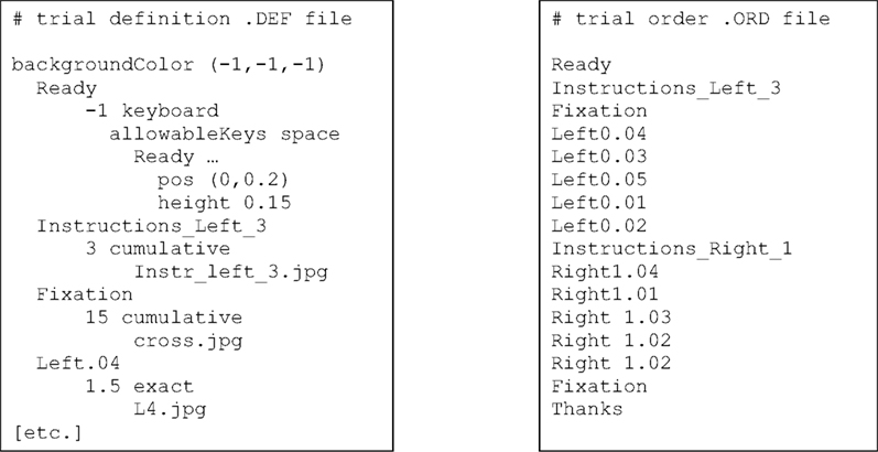
Figure 1. Abridged examples of the trial definition (.DEF) file format and the trial order (.ORD) file format. Each trial named in the .ORD file must be defined in the .DEF file. For the first trial (“Ready”), “timing = −1 keyboard” means wait indefinitely for a keypress (the spacebar is the only allowable key) while displaying the text “Ready …” at position (0,0.2) and height 0.15. The “Fixation” trial involves displaying the image file cross.jpg in the center of the screen for 15 s, with extra frames inserted or removed there if cumulative timing errors have accumulated. The “Left.04” stimulus displays the image file L4.jpg in the center of the screen for exactly 1.5 s.
The breadth of experimental designs commonly employed in functional neuroimaging experiments requires sophisticated and flexible procedures for trial scheduling. Possibilities for the temporal ordering of trials include: (i) block designs, in which groups of evenly spaced trials alternate with periods of fixation, (ii) stochastic, or “event-related”, designs, in which the individual trial times are varied to allow efficient estimation of hemodynamic responses using deconvolution procedures (Dale, 1999
), and (iii) mixed designs, combining aspects of both block and stochastic designs to achieve separation of state and task-related experimental effects. In the case of stochastic and mixed designs, the trial durations and orders that lead to maximum efficiency in the detection of task-related brain activity can be computed using programs such as optseq
3
, and then entered in a trial order (.ORD) file. As with the trial definition file, the trial order input file is a simple, ASCII file (Figure 1
, right). From these two input files (.DEF and .ORD), NinSTIM builds and then runs a PsychoPy-compatible program.
PsychoPy and Pyglet, the engines driving stimulus presentation, also provide facilities for logging stimulus, keyboard and mouse events. Through the Pyglet event loop, one can continuously monitor these events and respond appropriately. For example, one can display different stimuli depending on user input, or compensate for certain timing vagaries inherent in soft real-time operating systems. In soft real-time operating systems like Microsoft Windows, interrupts and system processes can sometimes seriously disrupt the accuracy and precision of stimulus timing. This is a widely recognized problem that is addressed using differing mechanisms in the stimulus presentation packages most commonly used in experimental neuroimaging, including EPrime
4
, Presentation
5
, Psychtoolbox
6
, and Cogent
7
. To optimize timing in NINstim we: (i) increase the stimulus display process priority to “High” via Python’s win32process.SetPriorityClass(), (ii) disable Python garbage collection, (iii) enable drawing synchronized to the vsync pulse from the monitor, and (iv) pre-draw stimuli whenever possible to maximally engage the blocking mode of calls to OpenGL flip (Straw, 2008
). Stimulus onset timestamps are collected using Python’s time.clock() call which is executed the line after the call to flip the OpenGL graphics buffer. The timing requested by the user in the trial definition and order files – which we call the nominal timing – is also simultaneously monitored. Using the “cumulative” timing type, users can identify the less critical stimulus or delay times, for which NinSTIM can add or subtract one or two frames, to preserve the experiment’s cumulative nominal timing. In a 12-h test using this approach, involving 15,600 trials and 31,000 stimuli, our time.clock() timestamps occurred a maximum of 26 ms early to 88 ms late compared to nominal, with a mean and SD timing error of 1.6 ± 6 ms. Individual stimulus durations ranged between ±8 ms off nominal – or half a screen refresh on our 60-Hz monitor. Note that these latencies do not represent the total system delay, defined as the interval between the time a user event is captured and a new image is displayed. Moreover, these latencies were measured by the internal computer clock, rather than an external source. Hence, the above numbers may underestimate the exact latency to stimulus presentation (Straw, 2008
). However, the maintenance of nominal timing within a few tens of milliseconds over several hours is more than adequate for functional neuroimaging experiments based on hemodynamic responses, which includes the vast majority of NIN experiments.
Using the standard Python threading and ctypes modules it is also possible to collect continuous data streams from other user input devices during stimulus display. Access to almost any device driver is possible through ctypes. By setting up a separate timer thread, densely sampled data streams from auxiliary input devices can include time stamps from the same master clock that marks all stimulus, keyboard and mouse events. This arrangement dramatically reduces the timing uncertainty between stimulus presentation and recording devices and can provide a record of any mismatch between intended and actual experimental event times. This sort of continuous, simultaneous recording of auxiliary devices can be difficult or impossible to implement using many of the popular experimental control programs. In addition, the pyserial and pyparallel Python modules (Liechti, 2008
) provide a separate means for acquiring event signals from, or exporting trigger signals to, the computer’s serial or parallel ports for synchronization with our NIN acquisition devices.
Because NinSTIM is based on Python, chaining multiple experiments is easily achieved with successive Python calls, or a separate Python script that runs each experiment in succession.
Data acquisition and real-time data display system (NinDAQ)
Optical imaging devices are constructed from multiple hardware subsystems that require dedicated device control software. Using Enthought’s Chaco/Traits modules (Enthought, 2007
, 2008
), along with NumPy (Oliphant, 2006
) and SciPy (Jones et al., 2001
) we have also developed NinDAQ, a device control program customized for two of our NIN instruments (Figure 2
). This program provides complete, real-time control over the NIN device state variables, including laser state, amplifier gain, analog acquisition subsystem voltage range, and sampling rate. NinDAQ also controls the data acquisition process including start signals, stop signals, and data display modes. Important additional features include: real-time temporal display of relatively large amounts of data, pushbutton toggling to “zoom in and out” on the data stream as it is being collected, and automatic scaling of the signal range to the minimum and maximum values of each data line. Real-time control of the acquisition process is provided, including provisions for user-generated interrupts of data collection, variable temporal windows for strip-chart data views, and interactive laser control. The Chaco plotting package provides real-time plotting capabilities, while Enthought’s Traits supports rapid GUI development cycles. The standard Python ctypes module enables seamless access from Python to the commercial drivers for our analog-to-digital data acquisition boards.
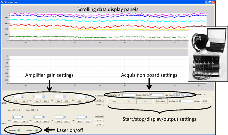
Figure 2. Screenshot from the NinDAQ device control and data acquisition program. Inset: The NIN recording devices and head probe being controlled by this software.
Signal Processing (NinPROC)
Once complete, most neuroimaging experiments produce two file types: text files that log the stimulus and response events, and custom binary data files containing the neuroimaging data. Depending on the type of experiment and the specific neuroimaging device, raw data from a single participant in single experimental session can be many gigabytes in size. In experiments incorporating cardiac, respiratory, kinematic or other physiological data monitoring, a third file type containing records of such continuous data streams may also be produced. Each such data file has unique processing requirements that can be handled via Python, or using the NumPy and SciPy libraries.
Quality assurance and filtering
Quality assurance procedures for stimulus and event log files involve validating event timing by examining deviations from nominal event times and durations, detection of skipped stimuli or skipped frames, detection of device failures, and identification of other experimental anomalies, including task performance deviations. Data quality checks can be easily implemented in Python by opening the log files generated by NinSTIM and NinDAQ, reading in each line with the recorded actual and nominal times, and computing various time differentials. NinPROC uses simple descriptive statistics to identify deviations from the expected experimental event timing, with relevant functions contained in NumPy (amin, amax, mean, std, or median) or scipy.stats (skew, kurtosis, or histogram). There is also an option to graphically display histograms to visually identify anomalous timing patterns during particular runs, using matplotlibhist() and plot() functions. For physiological or NIN data time series, numpy.loadtxt() or numpy.fromfile() can be used to efficiently read in the data, which can be similarly scanned for timing irregularities, intermittent signal dropout or other deviations from the experimental protocol. In addition, multiple time series can be quickly and automatically plotted with nindisp.plot() for visual inspection.
To identify and remove the sorts of signal artifacts specific to NIN data, we have included algorithms in NinPROC for semi-automated signal pruning. For a variety of reasons, not all source–detector pairs will provide useful information in all experiments. Data from some source–detector pairs not of primary interest may have been recorded during the experiment, some source–detector pairs may have been too far apart to provide reliable signals, or a detector may have lost contact with the head, thereby generating large signal artifacts. Within the preprocessing component NinPROC, the ninproc.prune() function is available to remove particular sources, detectors, or channels based on the known source–detector separations. In addition, low overall signal intensity can result in unreliable information, and high overall signal intensity can indicate light leakage from source to detector. Hence, facilities for displaying and pruning based on absolute signal intensity and signal-to-noise ratio (SNR) are also provided as options (Figure 3
). In addition, the ninproc.lowpass(), ninproc.highpass(), and ninproc.notch() functions provide simple, zero-phase filtering to reduce 1/f physiological, instrument, or electrical interference noise components.
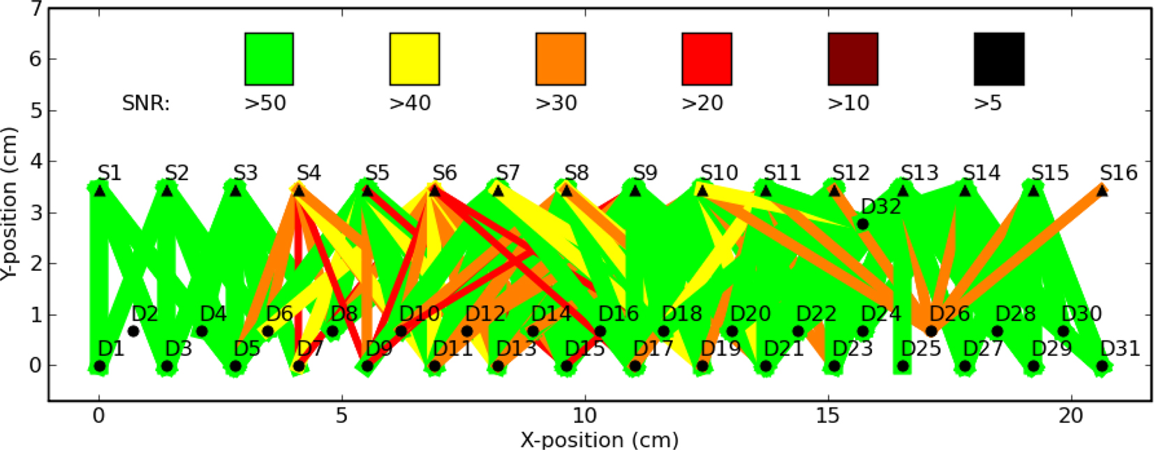
Figure 3. Graphical depiction of channel by channel SNR, computed as mean signal intensity divided by the SD of signal intensity over time (S = source position, D = detector position). Source–detector pairs with SNR > 50 are connected with green lines, while those with lower SNRs are connected with progressively darker lines. Sources or detectors with few or only bad connections (e.g., S16, D25) could be candidates for pruning. Regions of red colors indicate reduced sensitivity relative to other regions, as seen in the vicinity of sources S4 and S6.
As with all neuroimaging data, NIN time series can contain physiological motion artifacts. When head motion occurs, the resulting signal modulations can be substantial and therefore must be identified and either excluded or otherwise mitigated. Exclusion of a motion contaminated time series segment is a less than ideal solution, so effective mitigation is an important tool. One approach, which is particularly well-suited to real-time applications, is adaptive filtering. In previous work, we have demonstrated the efficacy of adaptive filtering to identify and reduce global physiological interference in NIN signals, including signal modulations resulting from cardiac or respiratory oscillations (Zhang et al., 2007a
,b
). We have recently added a least mean squares-based adaptive filter for motion artifact reduction to NinPy called ninproc.lms() (Figure 4
). Adaptive filtering has shown considerable promise in real-time reduction of physiological motion artifacts without the bandwidth loss associated with using a low-pass filter with a low cutoff frequency. Other published approaches to dealing with NIN motion artifacts include the use of principle component analysis or independent component analysis to identify and separate signal from motion waveforms (Morren et al., 2004
; Zhang et al., 2005
), solutions that could be incorporated using the Python-based Modular toolkit for Data Processing (Berkes et al., 2008
)
via mdp.pca() or mdp.fastica().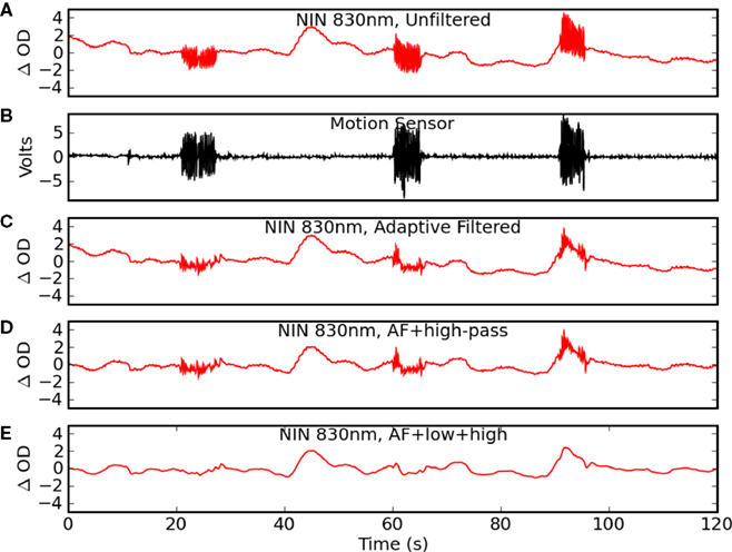
Figure 4. NIN data motion artifact reduction using NinPROC and adaptive filtering. Time courses are: (A) raw NIN data; (B) simultaneously acquired raw piezoelectric motion sensor data; (C) adaptively filtered NIN data, using (A) as the target and (B) as the reference signal; (D) signal in (C) plus a second-order Butterworth high-pass filter using scipy.lfilter() (cutoff = 0.05 Hz); (E) signal in (D) plus a sixth-order Butterworth low-pass filter using scipy.lfilter() (cutoff = 2 Hz).
Spectroscopic conversion
Table 1
lists multiple types of optical contrast detectible with NIN (Villringer and Chance, 1997
). Many of these contrasts are computed via spectroscopic conversion using the modified Beer–Lambert law (Delpy et al., 1988
). These conversions are linear algebra transformations performed on each time point of raw attenuation data and the resulting time series reflect time-varying changes in chromophore concentrations. To compute chromophore concentrations, raw measurements recorded from two or more NIR wavelengths are first log transformed to changes in optical density, and then to changes in O2Hb, HHb, and total hemoglobin (O2Hb + HHb) concentrations:
where I is the raw measured intensity at a single point in time, Io is the measured light intensity at a reference time point, ΔOD represents the change in optical density between I and Io, the ε()s are extinction coefficients for O2Hb and HHb at a given wavelength (λ), L is the source–detector separation, and DPF(λ) is the wavelength-dependent differential pathlength factor that converts L to the true (scattered) optical pathlength. Recording data from two wavelengths (λ1 and λ2) provides two such equations with two unknowns: the change in O2Hb and HHb concentrations. The ninproc.extinction_coef() function uses interpolated lookup tables to obtain extinction coefficients of the various optical chromophores. With these coefficients, conversion to concentrations over all time points can generally be accomplished compactly in Python using NumPy arrays, broadcasting, and its linear algebra capabilities, as shown in Code Fragment 1
, where
L is a 1D array of source–detector separations for each channel, rawdata is a 2D array of raw (or pruned and filtered) NIN data, rawref is a 1D array of raw NIN data from a reference period – e.g., N.mean(rawdata[:100],0), A is a linear transform between optical density and concentration represented as a 2D matrix of extinction coefficients, hhb and o2hb are 1D arrays of HHb and O2Hb concentrations (in units of moles/mm) over time. While A is normally invertible, sometimes it is not. For such cases, one can use numpy.linalg.pinv() in place of numpy.linalg.inv(). The results of these steps are shown in Figure 5
.
Code Fragment 1. Three lines to convert raw NIN data to oxygenation concentrations.
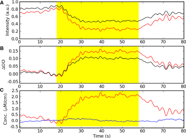
Figure 5. Spectroscopic conversion steps of NIN data time series from one source–detector pair. (A) Raw recorded NIN light intensity data from two wavelengths, in arbitrary units. (B) Data from (A) after log transformation to optical density units. (C) Data from (B) after conversion to hemoglobin concentration units (red = oxy-Hb, blue = deoxy-Hb, yellow = period of task activity).
Imaging (NinDISP)
Near-infrared measurements of brain function can be made with a single source–detector pair, providing information localized to approximately 0.5–1 cm2 of brain tissue (Strangman et al., 2003
). A spatially-distributed collection of such measurements can be combined into an image for each relevant optical contrast. In functional neuroimaging, task-related images of O2Hb, HHb and O2Hb + HHb changes are of primary interest, as these parameters have been shown to reflect underlying changes in neural activity (Jasdzewski et al., 2003
; Strangman et al., 2002b
). Imaging procedures can consist of topology preserving sensor space representations, back propagation – also called topographic imaging – or tomographic reconstructions (Arridge, 1999
), as discussed below.
Sensor space representations
Perhaps the simplest approach to imaging, commonly utilized in EEG and MEG data displays, involves plotting multiple sensor time series or time averages, with each sensor positioned in the display according to the scalp location of the measurement. An example of this approach from NinDISP, using the powerful matplotlib plotting package (Hunter, 2007
), appears in Figure 7
B. The surface array visualization technique preserves the temporal information at each sampling point, and is particularly effective if the sensors are widely separated.
Topographic imaging
In topographic imaging, measurements obtained from different locations in space are linearly interpolated to a regular grid to generate 2D images of either the underlying optical signal changes or derived parameters. The matplotlib.mlab.griddata() function can be used to compute such tomographic images. For example, if data is an N × 3 array of
[x,y,val] triples irregularly spaced over a 10 cm by 6 cm region, a 2D topographic projection of the val parameter with 1 mm pixels could be computed as follows (see Figure 7
C):
This is a simple and compact data visualization technique, but it also embodies many important assumptions. In particular, interpolation assumes that the time varying optical properties of brain tissue between measurement locations can be accurately estimated by averaging the signals derived from the neighboring actual measurements. This may or not be true depending on the spatial scales of the signal and the source–detector geometry. In the above example, it also assumes accurate prior knowledge of the (x,y) coordinates of the val parameter, which may be difficult to obtain or estimate. For simple geometries, however, this computationally efficient method is suitable for real-time display and can be quite useful for visualizing the spatiotemporal structure of signal modulations.
Tomographic imaging
Tomographic imaging, in contrast to topographic imaging, is more appropriate when multiple, spatially overlapping NIN measurements are collected. In this case, tomographic image reconstruction generates a solution that best satisfies all measurements simultaneously. The reconstruction is computed in two stages. First, one must estimate the diffusion paths of photons and calculate the sensitivity profile throughout the brain. In image reconstruction, this step is termed the “forward problem.” For simple, semi-infinite, homogeneous media, the distribution of photons injected into tissue can be approximated by the diffusion equation (Farrell et al., 1992
), and solved analytically. However, for more complicated geometries, analytical solutions are not possible and hence numerical solutions are often employed, including finite difference, finite element and Monte Carlo approaches (Jacques and Wang, 1995
). Here we discuss the Monte Carlo approach. For the particularly complex tissue geometry of the head, one can start with a standard high resolution, T1-weighted MRI scan (Figure 6
A). This structural scan can then be segmented into gray matter, white matter, cerebrospinal fluid, skull, and scalp tissue types using Python to call any of the MRI tissue segmentation tools contained in analysis packages such as SPM8
8
or FSL
9
. Next, each tissue type in the segmented volume is assumed to be homogeneous and assigned optical properties based on literature values (Choi et al., 2004
; Kohri et al., 2002
; Leung et al., 2005
; Okada and Delpy, 2003
; Strangman et al., 2003
).
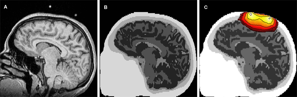
Figure 6. Simulated photon propagation through the head. (A) Typical anatomical MRI scan, with NIN sensor fiducial markers visible above the scalp. (B) Segmentation of the MRI scan in (A) into separate tissue types where Python was used to chain together the MRI segmentation modules. (C) Example photon densities for a single source–detector pair separated by 4 cm, overlaid on the segmented head. The colored areas delimit the region to which many NIN instruments would be sensitive, with a loss of 1 order of magnitude sensitivity per contour line. Images were generated using matplotlib.imshow(), NumPy masked arrays, and matplotlib.contour().
To perform the Monte Carlo simulation process, approximately 100 million photons are injected, one at a time, into the segmented model (Figure 6
B) at the location of a source or detector. The propagation of each photon through the tissue is determined probabilistically given the physics of light and the optical properties assigned to each tissue type. This process is repeated for each source and detector location and the result is a participant-specific solution to the forward problem. Multiplying together the photon densities for a given source–detector pair, point by point throughout the brain volume, provides an estimated sensitivity profile for that source–detector measurement pair (Figure 6
C). As with the MRI segmentation routines, Monte Carlo techniques can be implemented with Python calls to existing toolboxes in Matlab (Boas, 2004
) via mlabwrap (Schmolck, 2007
), or by calls to binaries such as tMCimg (Boas, 2008
) using Python’s os.popen() function. For NinPROC, and the steps in Figure 6
, we utilized the lattermost approach, which allows us to gradually transition complex code bases to Python, as time and resources permit.
Given a stable solution to the forward problem (Figure 6
C), the second imaging step is to generate an image of the optical contrast parameter. This step is called “inverse modeling”, and it can be accomplished using linear or non-linear methods. The linear approach is typically formulated as
y = Ax, where y is a length-M vector containing the value of the parameter of interest for each NIN source–detector pair, x is a length-N vector of all voxels in the image reconstruction, and A is the sensitivity matrix (Jacobian), which is an M × N matrix based on the Monte Carlo simulation that maps the sensitivity of each point in x to each measurement in y (Figure 6
C). To solve for x, the equation of interest becomes: x = A−1y, where A−1 computed using numpy.linalg.inv(A) or, more often, the pseudoinverse of A via numpy.linalg.pinv(A). Because this problem is usually ill-posed and underdetermined (N >> M), regularization is typically applied, often via singular value tapering as is used in Tikhonov regularization (Pogue et al., 1999b
). NIN image reconstruction then essentially reduces to two python function calls: matrix multiplication via numpy.dot() and regularization with numpy.linalg.svd().Statistical Modeling and Visualization
The final stage of an NIR functional imaging experiment, after completing the data collection and the signal and image processing steps, involves parameter estimation, statistical modeling, and visualization of the results.
Statistical modeling (NinSTAT)
Statistical modeling involves modeling experimental variance to derive parameter estimates pertaining to the experimental effects of interest. SciPy includes a number of basic statistical functions that are suitable for modeling experimental effects in individual subjects. However, data from many neuroimaging experiments, particularly those involving comparisons of different participant groups, have a complex and hierarchical variance structure that cannot be effectively modeled with SciPy routines. In particular, within-subject designs, incorporating repeated measurements collected from each participant under a range of experimental conditions are quite common. These designs are popular because they have relatively high sensitivity, and they avoid the time and expense of recruiting and fully characterizing large groups of research participants. Within-subject variability in functional neuroimaging data, while substantial, tends to be smaller than between-subject variability. Prominent sources of between-subject variation include: (i) brain size and shape differences, (ii) neurovascular coupling differences, (iii) task performance differences in accuracy or response time, and (iv) variation in the specific strategy used to perform the task. To accurately model both within- and between-subject effects, therefore, requires mixed-effects modeling techniques (combining fixed and random effects), which are not available in HomER or SciPy. In addition, given the great diversity in experimental designs employed in functional neuroimaging experiments, specifically coding each statistical model in Python would be associated with substantial effort. These reasons motivate integration with an external statistics package.
R is a widely-used, open-source, statistics package that contains a very comprehensive and sophisticated collection of statistical analysis methods (R Development Core Team, 2005
), including tools that are able to model NIN data with complex hierarchical structure. One common example is with mixed effects models that contain variables measured at different levels in a hierarchy, as in the case of summary statistic models in which separate regression analyses are computed for each participant, with the resulting first-level regression coefficients being treated as random variables at the second level (Pinheiro and Bates, 2000
). Rather than rewriting the requisite statistical procedures in Python, the RPy module (Moriera and Warnes, 2004
) provides a lightweight yet powerful interface between Python and R for statistical analysis, with results automatically returned to Python for storage, subsequent processing or display.
A particular advantage of using R is that an extremely broad range of models can be applied to the data, since all input variables are treated equally. In particular, the neuroimaging data can be used either as an outcome variable, a predictor, or a covariate. This assignment flexibility is in contrast to that found in the most commonly used neuroimaging software packages, including SPM, FSL, AFNI, FSFast. These packages require the neuroimaging variable to be the outcome variable, which significantly restricts the types of scientific questions that can be addressed. For example, one question that is receiving growing interest concerns identification of brain regions that might provide predictive information about treatment response. This determination requires the neuroimaging data to act as a predictor and the therapeutic response measure to serve as a dependent or outcome variable. Implementing these models using existing neuroimaging packages requires extracting the data from each potential brain region of interest, exporting the data series, and then performing the statistical analysis using an external program (Strangman et al., 2008
). By directly interfacing with R, one can fit predictive models as easily as those utilizing the image data as the dependent variable. Code Fragment 2
provides an example of a NinSTATS implementation of predictive modeling. Importantly, R includes a large, and continually growing, collection of heavily tested and more sophisticated models, including robust covariance and generalized linear models, as well as a wealth of post-hoc testing capabilities.
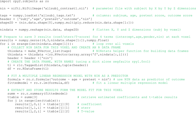
Code Fragment 2. NinSTATS code fragment to perform statistical analysis with functional NIN data as a predictor of outcome.
Visualization (NinDISP)
Once a neuroimaging statistical analysis is complete, visualization enhances both interpretation and communication of the results. Sensor space visualization, an approach discussed earlier, is shown in Figures 7
A,B. However, it is common in neuroimaging experiments to have even larger collections of spatially coherent univariate statistical results. For example, the code in Code Fragment 2
might produce 1,000 or more distinct model fits. In this case, sensor space visualization may be either impossible, because of too many measurements, or misleading, because overlapping measurements may be sensitive to different depths. Imaging provides certain advantages in these situations, as shown in the topographic image in Figure 7
C, generated from task-related regression parameters from the O2Hb traces in Figure 7
B. Applying a statistical threshold to topographic images helps identify regions that are significantly modulated by the task, as shown in Figure 7
D.
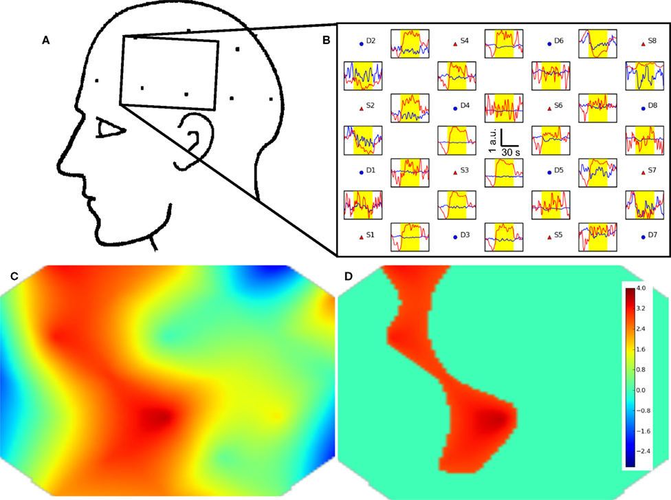
Figure 7. NIN data visualization. (A) Schematic of the NIN sensor region. (B) Sensor space display, with time series plots positioned at the source (Sx) and detector (Dx) locations. Individual time series plots show time on the x-axes and oxy-hemoglobin (red) and deoxy-hemoglobin (blue) concentrations on the y-axes. Yellow highlights the interval in which the subjects were engaged in a sequence learning task. A scale bar in the center indicates that the task period was 32 s in duration. Concentration is shown in arbitrary units (relative concentration), due to an unknown scattering factor. (C) Example NIN image of task-related oxy-hemoglobin regression parameter Z-scores from (B) corresponding to the rectangular area shown in (A). (D) The same data as (C), masked at a statistical threshold of p < 0.05 corrected for multiple comparisons. Color bar for Z-scores in both (C) and (D) appears in (D). Plots B–D were made with NinDISP using matplotlib.
In addition to statistical parametric maps (Figure 7
D), and time series plots (Figure 7
B) it is often useful to generate and examine scatter or bar plots from regions-of-interest, or to produce summary plots of activity levels in various brain regions, including histograms and box plots. The matplotlib module provides all these options as well as many additional plot types. Critically, matplotlib includes complete customization capabilities for the creation of publication-quality figures (Hunter, 2007
). Math or Greek symbols can be easily added to the plot or axis labels, options that are particularly important for representing physical or derived units in NIN data (cf. Figure 5
).
File Format Interfaces to Existing Optical Imaging Tools
Due to the large volume of spatial and temporal data generated by neuroimaging experiments, neuroimaging data have always required custom file formats, and in the 1990s image file formats proliferated. Fortunately, the NIfTI standard (Cox et al., 2004
) has made major inroads as a standard file format for MRI data. An example of its use in NinPy is seen in Code Fragment 2
. Other formats still dominate in EEG, MEG, PET, as well as NIN, and a number of legacy formats still persist with some frequency in MRI applications. Our goal has been to integrate NinPy programs with three key data formats: NIfTI, the Matlab-based format used by HomER (Huppert, 2006
), and the broad standard HDF5. These formats enable broad interoperability of the NinPy suite with existing tools for neuroimaging data analysis. NIfTI files are created, read and written through the use of the PyNIfTI package (Hanke, 2008
), whereas the HomER file format can be read and written as a Matlab.mat file or HDF5 file (also readable by Matlab) containing multiple arrays with specific variable names. Reading and writing Matlab files is supported through scipy.io.loadmat() and scipy.io.savemat(), and thus HomER files can be saved from appropriate variables in Python as follows:

Multimodal Integration
While we have only briefly discussed MRI integration with regard to Monte Carlo simulation, there are additional advantages associated with integrating NIN with MRI and other neuroimaging modalities. For example, the segmented MRI images (Figure 6
B) could be used to constrain the NIN image reconstruction process by restricting reconstructed brain activity modulations to gray matter, thereby not allowing the estimated signal changes to occur in scalp, skull, cerebrospinal, or white matter tissue compartments. As another example, automatic identification of optical sources and detectors within the MRI space (the white fiducial markers above the head in Figure 6
A) could be used as inputs to the Monte Carlo simulations or to provide more accurate co-registration of NIN statistical parametric maps with underlying brain anatomy.
While integration with EEG, MEG, and other neuroimaging technologies is occurring at the experimental level, integration at the data analysis and interpretation levels is a relatively underdeveloped area. One interesting possibility for integration involves the optical “fast signal”. NIN studies from several labs have shown changes in non-invasive optical signals on timescales much faster than typical hemodynamic changes, less than 100 ms as compared to 2–3 s or more (Franceschini and Boas, 2004
; Gratton et al., 1997
; Morren et al., 2004
). Since the nature of this fast NIN signal is an area of active investigation, close integration of NIN measurements with more direct EEG and MEG measurements of neuronal activity could lead to a fuller understanding of the nature of this optical fast signal. Integration with new, high-speed, MRI acquisition techniques (Lin et al., 2008a
,b
) may also help shed light on the nature of this optical fast signal and whether or not there might be analogous fast hemodynamic signal modulations detectable using MRI.
Advanced Volume Visualization
Combining structural and functional neuroimaging results requires advanced volume visualization tools. Thus far, we have sought to capitalize on the popularity of the NIfTI file format, as it allows convenient utilization of a range of existing MRI 3D visualization packages. However, with the development of Python neuroimaging tools such as NiPy (NiPy Development Team, 2006
), as well as the impressive capabilities afforded by Python bindings to both the Visualization Toolkit (via vtk’s own Python bindings, or via Enthought’s tvtk) and OpenGL (via PyOpenGL), adding native Python 3D visualization for neuroimaging is expected in the near future. Incorporating 3D display capabilities in NinPy would facilitate the sorts of flexible and customized visualization often absent in existing packages. Visualization in three dimensions is often critical to developing better insights into the structure of high-dimensional datasets. The ease with which customization can be made with Python scripting, coupled to a high-level visualization package, is expected to be widely adopted in a broad array of neuroimaging data visualization applications.
The relatively short time needed to construct the NinPy suite of tools was made possible given the substantial prior efforts reflected in the packages listed in Table 3
. Thanks to these developments, we can foresee completion of an end-to-end, Python solution for developing, conducting, analyzing and displaying the results of NIN experiments. Key enabling technologies that have appeared over the past few years include the stabilization of numeric arrays and processing (NumPy), the advancement and continuing stabilization of a broad base of scientific algorithms (SciPy), the development of a robust interface to the R statistical modeling package (RPy), and substantial advances in the mechanisms for stimulus, array and volume visualization (e.g., PsychoPy, Matplotlib and Chaco). We have found that the use of Python as the core programming language for our NIN programs provides significantly better control over most aspects of an NIN experiment than is possible with existing packages. Importantly, our development efforts have not required any time-consuming coding or debugging in C, nor do users need to learn multiple programming or scripting languages to complete a functional neuroimaging experiment. We have found that, particularly for complex problems including optical image reconstruction, hierarchical statistical analysis, or volume visualization, Python can serve as a convenient, powerful, and maintainable scripting “glue”. This architecture allows us to rapidly deploy an operational end-to-end Python solution, allowing later conversion of non-Python algorithms as resources and motivation permit. Reducing our dependence on multiple separate software tools or programming languages for stimulus presentation, data acquisition, data analysis, image reconstruction, statistical modeling, and graphical display greatly simplifies the experimental working environment, and has substantially increased scientific productivity. In addition, the single-language solution facilitates the development and distribution of easy-to-use, self-contained packages for conducting NIN experiments in mobile or remote settings where a dedicated experimenter may not be available. As more open-source tools are ported to Python, further improvements in productivity are envisioned.
We are releasing the source code for all of the NinPy modules for unrestricted use as each sub-module reaches beta level software quality. Completed modules will be available under BSD licensing
10
, or by contacting the authors.
Quan Zhang and Gary E. Strangman have a patent pending on technologies related to mobile neuroimaging.
We would like to acknowledge support from the National Space Biomedical Research Institute through NASA Cooperative Agreement NCC 9-58.
- ^ http://www.pyglet.org
- ^ http://www.psychopy.org
- ^ http://surfer.nmr.mgh.harvard.edu/optseq/
- ^ http://www.pstnet.com/products/e-prime
- ^ http://www.neurobs.com
- ^ http://psychtoolbox.org/PTB-2/
- ^ http://www.vislab.ucl.ac.uk/cogent.php
- ^ http://www.fil.ion.ucl.ac.uk/spm
- ^ http://www.fmrib.ox.ac.uk/fsl
- ^ http://www.nmr.mgh.harvard.edu/Neural_Systems_Group/software.html
Berkes, P., Wilbert, N., and Zito, T. (2008). Modular toolkit for data processing (version 2.3). Available at: http://mdp-toolkit.sourceforge.net
(Retrieved September 2, 2008).
Boas, D. A. (2004). Photon migration imaging toolbox. Available at: http://www.nmr.mgh.harvard.edu/PMI/resources/tmcimg/index.htm
(Retrieved August 25, 2008).
Boas, D. A. (2008). Monte Carlo photon transport. Available at: http://www.nmr.mgh.harvard.edu/PMI/resources/tmcimg/index.htm
(Retrieved August 25, 2008).
Cox, R. W., Ashburner, J., Breman, H., Fissell, K., Haselgrove, C., Holmes, C. J., Lancaster, J. L., Rex, D. E., Smith, S. M., Woodward, J. B., and Strother, S. C. (2004). A (sort of) new image data format standard: NIfTI-1. 10th Annual Meeting of the Organization for Human Brain Mapping, Budapest, Hungary.
Enthought (2007). Chaco. Available at: http://code.enthought.com/chaco/
(Retrieved August 25, 2008).
Enthought (2008). Traits. Available at: http://code.enthought.com/projects/traits/
(Retrieved August 25, 2008).
Gratton, G., Fabiani, M., Corballis, P. M., Hood, D. C., Goodman-Wood, M. R., Hirsch, J., Kim, K., Friedman, D., and Gratton, E. (1997). Fast and localized event-related optical signals (EROS) in the human occipital cortex: comparisons with the visual evoked potential and fMRI. Neuroimage 6, 168–180.
Hanke, M. (2008). PyNifti – Python-style access to NIfTI and ANALYZE files. Available at: http://niftilib.sourceforge.net/pynifti/
(Retrieved August 25, 2008).
Huppert, T. J. (2006). HomER. Available at: http://www.nmr.mgh.harvard.edu/DOT/resources/homer/home.htm
(Retrieved September 2, 2008).
Jones, E., Oliphant, T., Peterson, P., et al. (2001). SciPy: open source scientific tools for python. Available at: http://www.scipy.org
(Retrieved August 25, 2008).
Liechti, C. (2008). pySerial/pyParallel. Available at: http://pyserial.wiki.sourceforge.net/pySerial
(Retrieved August 25, 2008).
Moriera, W., and Warnes, G. R. (2004). Rpy, a robust Python interface to the R Programming Language. Available at: http://rpy.sourceforge.net/
(Retrieved September 2, 2008).
Morren, G., Wolf, U., Lemmerling, P., Wolf, M., Choi, J. H., Gratton, E., De Lathauwer, L., and Van Huffel, S. (2004). Detection of fast neuronal signals in the motor cortex from functional near infrared spectroscopy measurements using independent component analysis. Med. Biol. Eng. Comput. 42, 92–99.
NiPy Development Team (2006). NiPy: neuroimaging tools for python. Available at: http://neuroimaging.scipy.org
(Retrieved September 2, 2008).
R Development Core Team (2005). R: a language and environment for statistical computing. Available at: http://www.R-project.org
(Retrieved August 25, 2008).
Schmolck, A. (2007). Mlabwrap v1.0. Available at: http://mlabwrap.sourceforge.net/
(Retrieved August 25, 2008).
Strangman, G. E., O’Neil-Pirozzi, T. M., Goldstein, R., Kelkar, K., Katz, D. I., Burke, D., Rauch, S. L., Savage, C. R., and Glenn, M. B. (2008). Prediction of memory rehabilitation outcomes in traumatic brain injury by using functional magnetic resonance imaging. Arch. Phys. Med. Rehabil. 89, 974–981.