Brainlab: a Python toolkit to aid in the design, simulation, and analysis of spiking neural networks with the NeoCortical Simulator
1
Brain Computation Laboratory, University of Nevada, Reno, USA
2
Program in Biomedical Engineering, University of Nevada, Reno, USA
3
Department of Medicine and Program in Biomedical Engineering, University of Nevada, Reno, USA
Neuroscience modeling experiments often involve multiple complex neural network and cell model variants, complex input stimuli and input protocols, followed by complex data analysis. Coordinating all this complexity becomes a central difficulty for the experimenter. The Python programming language, along with its extensive library packages, has emerged as a leading “glue” tool for managing all sorts of complex programmatic tasks. This paper describes a toolkit called Brainlab, written in Python, that leverages Python’s strengths for the task of managing the general complexity of neuroscience modeling experiments. Brainlab was also designed to overcome the major difficulties of working with the NCS (NeoCortical Simulator) environment in particular. Brainlab is an integrated model-building, experimentation, and data analysis environment for the powerful parallel spiking neural network simulator system NCS.
Spiking neural network simulator software systems continue to grow in speed and capacity (see Brette et al., 2007
for a recent survey). The complexity and size of the models simulated on these systems also continue to grow, threatening to overwhelm the ability of the experimenter to build the models, conduct parameterized experiments, and analyze the huge amounts of resulting data. The simulators themselves are generally extremely efficient but minimalist tools written in low-level programming languages that are difficult to understand and modify by any but a few dedicated experts. Tools beyond the simulators themselves are needed to help the experimenter cope with the complexity of the experiments.
In our work with one such powerful spiking neural network simulator called NCS
1
(the NeoCortical Simulator, described briefly in the Section “NCS”) we encountered these general complexity barriers. Our work was also hampered by problems specific to working with NCS, most notably the necessity of preparing network models for simulation using NCS’s restrictive neural modeling interface, the
.in file format. We confronted all these problems together by creating a unified Python toolkit called Brainlab
2
, which has greatly eased the burden of organizing and conducting our experiments in general, and working with NCS in particular.The fundamental proposition of Brainlab is this: For the tasks of complex neuroscience model-building, experimentation, and analysis, nothing short of a full-fledged programming language will suffice. No neural model file format or restricted special purpose programming language for modeling will ultimately suffice for day to day work. And as long as a real programming language will be needed to hold the whole experimental enterprise together, it might as well be a modern mature programming language with a large scientific user community, rather than a custom-built, special purpose language. In Brainlab we selected the Python language for this purpose, and the rationale for our decision is given in the Section “Why Python?”.
Brainlab has been in use since 2003, with publications in 2005 (Drewes, 2005a
,b
). In the intervening time, validation for the decisions we made in the design of Brainlab seems to have come from several areas. Scientific support for Python, in the form of libraries and the user community, has continued to grow and mature. Other projects have independently started that also use Python as a front-end modeling and back-end analysis tool for various other neural simulators. The NEST simulator
3
system now offers a Python interface called PyNEST
4
. The NEURON
5
simulator has added Python as an alternative interpreter to Hoc. PyGENESIS is now available for the GENESIS
6
simulator. The PyNN
7
system, part of the broader Neuralensemble initiative
8
, goes a step further and offers a common Python interface to NEURON, NEST, and PCSIM
9
(but not NCS).
The Brian
10
project differs from the systems mentioned so far, and also NCS, in that Brian is a self-contained Python neural simulation solution, rather than a front-end to a simulation engine written in a different programming environment. Brian still achieves good single-processor simulation performance through the use of vectorized processing provided by the NumPy library, and it can also manage multiple jobs in parallel on a cluster computer system, but splitting a single large simulation onto multiple compute nodes is not supported. The Topographica
11
project provides standalone Python tools intended for exploring higher-level neural abstractions like sheets and projections from neural area to area. Though not primarily intended for investigations that require detailed simulation of individual neurons, Topographica can be interfaced to lower-level simulators like NEURON and GENESIS. Topographica is one of the older Python neuroscience tool packages, with an initial public release in late 2005.
Perhaps because NCS has a fraction of the number of users of some other simulators (e.g. NEURON and GENESIS), Brainlab has attracted comparatively little attention. Brainlab merited brief mention in a recent survey of major spiking neural net simulator packages (Brette et al., 2007
). Brainlab was unnoticed by another recent survey of interoperability of neuroscience software (Cannon et al., 2007
) though Python interfaces to other spiking neural network simulators (e.g. NEURON’s and NEST’s) were described there in some detail.
In this section, we will first describe enough about NCS so that a reader will understand the problems we faced designing a system to interface to and control it. Next we will describe the broad features we wanted to include in our toolkit, and how we wanted the finished system to appear to the user for modeling, simulation, and analysis. Then we will describe in detail how we actually confronted the problems interfacing to NCS, to implement the Brainlab system.
NCS
The development history of NCS is recounted elsewhere (Drewes, 2005b
). In its current evolution, NCS is a parallel (MPI-based) spiking neural network simulator written in C/C++ that can perform very large discrete-time simulations with a reasonably high degree of biological realism. Simulations with a million neurons and a billion synapses have been accomplished. NCS allows for neuron models that include detailed and customizable ion channel and cell membrane voltage dynamics, but for efficiency the stereotypical action potential voltage and postsynaptic conductivity waveforms are templated rather than generated dynamically. NCS supports multi-compartment cells but often large scale simulations are done using single compartment models. A good recent comparison of NCS with other spiking neural network simulators, including some discussion of maximum simulation sizes, is Brette et al. (2007)
.
The NCS Input File (the .in File)
NCS reads a description of a neural network model and other simulation parameters from a plain text file whose filename is supplied to NCS as a command line argument. For our purposes here it is not necessary to go into great detail about the format of this file, but we do wish to describe it generally in order to explain some of the shortcomings of working with it.
This input file, hereafter called a
.in file after the convention of using .in as a filename extension for such files, contains a variable number of subsections. Each subsection starts with a line that contains the name of the subsection (which must be one of a limited number of keywords permitted by the system) and ends with a line that contains END_ with the section name appended. The first subsection in a .in file is the BRAIN section. In the BRAIN section of the file are defined global features that affect the entire simulation. For example, a line beginning with JOB defines a job name for the simulation. Some subsections can be repeated (for example, a COLUMN or LAYER), and then each is assigned a unique text identifier within the file. The file format allows other portions of the file to reference these named objects, to create additional instances of them, but no structural or other significant variation in a defined object is permitted. The .in format definition permits no looping constructs or macro substitutions. Other sections of the .in file define connections between these objects, with references to the text names of the objects being connected. Because of these restrictions, NCS .in files tend to be quite long even for fairly simple networks, and they tend to be prone to syntactical error or internal referential inconsistency when edited manually.Other neural simulator systems acquired programming languages (e.g. Hoc for NEURON) to avoid the limitations of a flat input file format like NCS’s. NCS never went this far, though there were several attempts to elaborate the
.in file with macros, loops and other features. None of these efforts for NCS were widely used or reached the generality of a true programming language. Many NCS users eventually created custom text processing programs in other programming languages (like MATLAB) that would emit .in files. But writing special-purpose macro processors to create .in files is time consuming work that generally cannot be reused on later projects, and MATLAB is not a particularly good text processing tool. The experimentation process was either not automated or automated with external custom scripts, making the whole process cumbersome and systematic model parameter search difficult. Data file management was typically done manually using ftp type tools.One other unusual aspect of NCS deserves mention: it imposes a notion of the cortical column and the cortical layer as structural elements, and this requirement is reflected in the structure of the NCS input file. Even if an NCS user wishes to simply simulate two connected cells, or a homogeneous collection of cells for a study of, say, synfire chains, he must define those cells within an NCS LAYER text block, and that in turn within an NCS COLUMN text block. This introduces additional complication for the simplest simulations.
NCS Usage
NCS is optimized for large cluster computer systems (Beowulf clusters). A common usage pattern is as follows: A user typically first prepares an input file in the
.in file format in a text editor, specifying the neuron, synapse, channel, and network model. This file is copied across a network to the cluster computer and NCS is invoked there with the file as a command line argument. Reports are written to the cluster computer’s disks during the simulation run, which can last from a few seconds to days. Data analysis is then performed on the cluster computer if the data set is very large, or the data is copied back to the user’s workstation for data analysis if that is feasible. The experimenter then makes some adjustments to the model and tries again.Brainlab Motivation and Design Goals
Faced with the powerful but difficult to use NCS simulator, we set about to design a toolkit that would offer the following:
1. An interactive shell for simple experimentation with NCS, making NCS a more suitable educational tool for learning the behavior of spiking neural networks and also a more convenient platform for experienced users to explore the behavior of new cell or network elements.
2. A convenient platform for parameterized control of sets of NCS experiments.
3. A convenient platform for scripted regression testing of NCS itself, with flexible output validation.
4. Scripted, algorithmic generation of neural network models rather than NCS’s native static file specification of networks.
5. Convenient, integrated, graphical on-line reporting and plotting of spiking, current, and voltage activity of cells, synapses, and channels.
6. Convenient, integrated, on-line three-dimensional plotting of neural network architecture for expository and diagnostic purposes.
7. Experimental support for higher-level abstractions than those provided natively in NCS (for example support for areas, composed of arrays of columns, and a variety of distinct area-to-area synaptic connection patterns), and a flexible environment to add new ones.
8. Support for lower-level abstractions too unwieldy to reasonably manage in native NCS (for example, columns where all cells are enumerated and independently, rather than just statistically, addressable).
9. A container for a standard and extensible library of NCS network building blocks (for example channels, cell types, columns, spike templates), where all components are guaranteed to interoperate, utilize consistent naming conventions, and may be manipulated programmatically as variable objects rather than text chunks.
10. A more convenient, higher-level, object-oriented representation of neural networks that hides many complexities and inconveniences inherent in NCS’s native
.in file format.11. A convenient environment in which to convert a neural network description into a chromosomal representation suitable for use with a genetic algorithm.
12. A convenient environment in which to access NCS’s realtime stimulus input capabilities, especially for robotic interface applications (see Goodman et al., 2008
for more information on using NCS in robotics).
13. The ability to conveniently extend many of these capabilities without recourse to coding in NCS’s native compiled programming environment (the C/C++ language).
Why Python?
When we selected Python as the language for Brainlab, Python was not yet in wide use in neuroscience, and it was also in the midst of a seemingly endless reorganization of its vector processing math support libraries. Nevertheless, there were hopeful signs of building momentum for Python as a scientific platform, and the base language was so appealing in several respects that we selected Python as the language for our project.
Python is an open source, cross platform programming language. The base Python language is constantly being extended and made more powerful by hundreds of developers working together across the world. In addition to the base language, there are dozens of external packages in various states of development, from polished to prototype. These packages gradually move into the base distribution as they mature and if they are of sufficiently wide interest.
Python is ordinarily compiled into bytecode automatically and the bytecode is then interpreted in a runtime virtual machine. This is essentially the same approach used by Java, though the compilation generally requires an explicit step with Java. Compilation to bytecode results in code execution that is generally faster than ordinary interpreted code. Python is dynamically typed, making programming extremely convenient. Built in datastructures like lists, dictionaries (hashes), and arrays help make Python programs very concise. The clean syntax makes programs easy to understand. Python has a well deserved reputation as an extremely clean and easy to read and understand language.
At the time we selected it, Python already had a growing set of support library packages for scientific computation. These have since matured. Some of these packages are used in Brainlab, including:
• Matplotlib
12
, a MATLAB-like plotting package
• PyOpenGL
13
, OpenGL bindings for Python
• NumPy
14
, MATLAB-style array processing
• SciPy
15
, a set of scientific tools for Python, including pseudo random number generators and transforms
Brainlab to NCS Interface for Network Modeling
When we were designing the Python to NCS interface for the first version of Brainlab, there were already a number of ways to interface Python to a C/C++ application. Of these, one approach we considered seriously was to create a Python module out of the NCS C/C++ program with fairly simple and standardized wrapper code using standard techniques
16
. The wrapped C code could then be included into a Python program with the
import command. With this approach the Python program would be in charge from the beginning, and it could selectively make normal looking Python function calls into the wrapped C code to actually perform the NCS simulation and other functions. How would the network, cell, synapse, and other neural network parameters be communicated to NCS? A reasonable approach would be to define a new abstract network modeling interface using high-level Python facilities, perhaps a Python Object class for a Cell, a Synapse, and so on, that allows these objects to be created and interconnected. This Python-based model could then be converted directly to the internal in-memory representation of network models of NCS, called the GCList, through a new function provided by the imported NCS python module. This function, being in the C/C++ side of things, would have full access to the memory structures, memory allocation, and cluster-distribution routines that NCS itself uses to convert the .in file representation into the GCList representation for simulation, merely bypassing the file parsing NCS normally uses to build its internal network representation.However this tightly integrated approach would have a number of disadvantages. Such a Brainlab system would have to be at least recompiled with every new release of NCS. But there would be more complications than just that. While the NCS
.in file representation is part of the NCS documentation and is fairly stable, the internal GCList representation does not have a publicly documented interface. The GCList interface changes over time, and when it changes, corresponding detailed C/C++ changes would then have to be made in the NCS/Python module for import. A possibly larger documentation burden also would be placed on Brainlab to describe the new model-building interface.We opted instead to try to achieve our design goals with a much looser Brainlab-NCS interface for modeling and simulation. We left NCS as a completely separate programming project and did not even try to integrate more tightly with it than its existing published modeling (
.in file) and invocation (command line) interface. So Brainlab would have to provide a convenient and powerful Pythonic network modeling interface to the user, since that was a primary design goal, but it would also have to emit a properly formatted .in file for use by NCS on the back-end. The approach we took to model-building in Brainlab is depicted in Figure 1
.
Figure 1. Brainlab’s approach to building neural network models for NCS. A script using the Brainlab
brain.py module allocates objects of special modeling object classes (BRAIN, CELL, SYNAPSE, etc.) defined in brain.py. These objects each contain a Python dictionary called parms containing (name, value) pairs. Each such name corresponds exactly to an NCS character string parameter name for that record type within the .in file. Each value contains either the literal value desired for that parameter, or a Python object that will later be dereferenced and substituted with an appropriate text name for the text section representing that object in the resulting NCS .in file. The lower-level objects can be inserted into the higher-level objects through direct manipulation of the parms dict, but generally they are added there implicitly through the brain.py module’s helper functions such as BRAIN.AddColumn(). The value of the highest level container object, the BRAIN object, is determined by the overridden --repr--() function, which converts the in-memory model representation into the text .in representation, in the manner described in the text. The result is a Python character string which is a suitable input file for the NCS program.The
BRAIN, CELL, LAYER, and other sections of the NCS .in file are each implemented in Brainlab as a Python object class. The --repr--() method for each object is overridden so that printing an object results in text for that object in a format suitable for inclusion in the NCS .in file. In the case of a lower-level object, this method just prints out the object itself, but does not print any other objects that are referenced by the object being printed. The BRAIN object’s --repr--() method, however, first recursively traverses the entire tree of objects referenced from the BRAIN object and a list is composed for each type of referenced object. Once all referenced objects have been collected together, the entire NCS .in file is printed, starting with the BRAIN section, and proceeding to all of the other sections of the .in file in the conventional order.The lower-level classes are implemented as nested classes within the
BRAIN class. Note that they are not derived subclasses, but rather nested classes. Derived subclasses are appropriate where the subclass has most of the aspects of the superclass but some additional features. In Brainlab the nested classes are not logically subclasses of the BRAIN since they do not share the same characteristics as the super-object but are merely contained by it. However, the lower-level classes do need access to the component type libraries that are stored with the BRAIN class. If the lower-level objects were entirely separate classes, they would not have convenient access to the component type libraries. By making the lower-level classes nested within the BRAIN class, they do have that access.We chose to map many of the modeling details of Brainlab directly onto the underlying NCS implementation, rather than providing a completely new modeling interface. This primarily means that we preserve NCS’s text character string names for various neural parameters of the cells, synapses, channels, and so on. This eases the documentation burden on Brainlab since we can refer directly to the NCS’s documentation on many points. Furthermore, it makes keeping Brainlab up to date with respect with NCS very easy. Whenever NCS adds support for a new parameter within an existing modeling object, it is usually a simple matter to add it to the permitted parameter list of the appropriate class in
brain.py and that is the end of it. (When NCS adds entirely new types of objects, as is occasionally done, there is a bit more work, but even still it is usually just a matter of intelligently cloning an existing object to a new name and making a few changes.) The overall mechanism of .in file emission through recursive application of --repr--()’s to discovered objects starting at the top-level BRAIN extends quite easily.The simple strategies of creating a Python object class for each
.in file section, with automatic conversion from object to text through the --repr--() method, combined with the ability to reference one object from another, achieved all our design goals for a Pythonic modeling interface to NCS. The modeling power achieved by combining these few concepts in this way should not be underestimated.Brainlab to NCS Interface for Simulation
Once the internal Pythonic neural network model is constructed inside the top-level
BRAIN object, it can be simulated by invoking the BRAIN’s Run() method. Since we elected to keep an arms-length interface between Brainlab and NCS, the invocation of NCS is done through the use of a popen() call, as follows. First, Brainlab determines through invocation options or a standard configuration .rc file whether the NCS process is to be invoked locally, or on a remote compute server (typically a cluster). The .in file generated from the --repr--() method of the top-level BRAIN object is stored in a disk file locally, then propagated to the remote compute server using ssh
17
(secure shell) if necessary. Other support files, such as input stimulus patterns, are likewise generated and propagated as needed. Next, the NCS invocation command is constructed, again with appropriate references to remote servers with ssh, and then this command is executed using popen(). Brainlab monitors the realtime progress of the command as NCS reports the progress of the run through the file descriptors of the popen(). If an error condition is detected in the output, Brainlab either throws a Python exception, or an error code to the caller. When Brainlab detects that a run has completed, it constructs additional commands to retrieve output files from the remote compute server, as needed.We felt it was essential to support all three stages of operation – model-building, simulation, and analysis – completely within the control of the Python Brainlab environment. This permits self-contained and reproducible experiments, in the form of Python Brainlab scripts. This also opens up the possibility of parameterized model search with feedback from model performance affecting parameters of the next iteration, or even the use of genetic programming techniques for parameter search, all within a Brainlab script.
Brainlab’s Module Organization
Brainlab itself is implemented as two main Python modules,
brainlab.py and brain.py. The brain.py module contains the parts of the system concerned with building a neural model using Python classes supplied by the module and other normal Python facilities, and then automatically converting this model to a format understandable to NCS (a .in file). The brainlab.py module contains support functions for invoking an NCS simulation on a model either locally or remotely on a remote cluster, and analyzing and documenting the results using plotting and other functions.In addition to these two main modules, an optional module called
netplot is available. This module can take a model built using the core BRAIN class of brain.py and convert it into a three-dimensional depiction using the model’s architecture and hints provided during model construction. The three-dimensional depiction can be examined and explored interactively on a workstation or saved in a number of graphics file formats. The PyOpenGL
18
package is used for the actual rendering.Building Models with Brainlab
In Brainlab, every brain model is an instance of a new Python object class called
BRAIN. Once the brainlab library itself is brought into a Python program with the import command, creating a brain object is by the usual Python means:
The variable
b then refers to the newly created, and initially empty, brain model. When a BRAIN object is created, it contains a default set of commonly used types of neural network modeling components. (There are initially no instances of these types in the brain model.) These component types can be directly instantiated and then used for construction of network models, or they can be modified in place and then used in a model, or they can be copied to new types with different names and then the copies can be modified and instantiated for use in a model. The component types are contained in Python dictionaries (hashes), and the keys of the dictionary are simply the text names of the components. These building blocks are automatically included within a Python dictionary called libs in each BRAIN instance. There can be multiple libraries of parts within a BRAIN. The library provided with the class is given the key name standard, and is itself a dictionary. In this dictionary are subdictionaries for the different types of neural modeling components, such as channels (accessed with the chantypes dictionary key), cell types (accessed with the celltypes key), synapse facilitation and depression profiles (under the sfds key), and more as listed below.The following interactive Python session shows how to view these different library components and shows how one could modify the negative Hebbian learning window duration parameter within the standard Hebbian learning profile:
The Section “Usage Example: RAIN Network” contains another example of creating components based on the included standard library.
An NCS
.in file contains a number of text blocks, with each block consisting of a number of parameter keywords on the left and their values to the right. The values can be of several types. In the example above, the numbers for the NEG_HEB_WINDOW are a mean and standard deviation. During model initialization, NCS assigns that parameter to a random value from a normal distribution with the mean and standard deviation requested. For other parameters, such as the RSE_INIT parameter of the synapse object, two numeric values specify a minimum and a maximum of a range. In the case of the LEARNING parameter in the example above, the value for a parameter is a text label that references another block defined within the file. The NCS documentation details each parameter and its expected values. In some cases, Brainlab allows commonly used and frequently modified parameter values to be changed in Brainlab function calls. For example, when specifying a synaptic connection, the probability of the connection and the conductance speed values can be set directly using the prob= and speed= keyword arguments to the Brainlab AddConnect() method. In all cases however, NCS parameters can be set by modifying a dictionary value in the appropriate parms dictionary of the object with the key set to the text name of the NCS parameter name. This approach gives convenience to the programmer while allowing quick access to new NCS parameters as they are added to the system, by simply adding a keyword to a list in the Python class definition for that object.In NCS, cells cannot exist on their own but rather only as part of a higher-level structure called a column. A column is composed of one or more layers, which in turn is composed of one or more groups of cells. Brainlab has
COLUMN, LAYER, and CELL objects that correspond to these structures. A Brainlab script can build a column up from cell groups and layers, or instead use a convenience function that will add a pre-built column in a single step. The following Brainlab function adds to the model an instance of an ordinary column populated with a single cell:
Additional optional parameters to the function can specify a cell type to use (other than the default), spatial coordinates for the cell, and more.
At this point the Brainlab script typically makes connections between the cells or cell groups. Brainlab functions such as
AddConnect() are used for this. The Python variables for the objects are used as the point of contact for connection. An example of this is given in the Sections “Usage Example: Hebbian Learning” and “Usage Example: RAIN Network”. Report requests are also added to the brain at this time.Simulating Models with Brainlab
Once the
BRAIN object is created, simply printing it with the Python print command causes Brainlab to emit a complete, properly formatted .in file containing all the information added to the brain by the modeler. If desired, this file can be examined and manually submitted for simulation by NCS. This approach is occasionally useful for debugging purposes, but in practice it is seldom necessary to view the generated .in file directly. Instead, the modeler can simply leave the underlying .in file mechanism hidden and evoke an NCS simulation directly on the model using the brainlab Run() function on the brain:
In this example the simulation is evoked remotely on 32 processors. The
.in file that results from the model is created by Brainlab behind the scenes, copied over to the compute cluster automatically by Brainlab, and the simulation results are fetched on demand as the data analysis portion of the Brainlab program requires them.Brainlab is designed primarily to run on the user’s workstation, and send jobs across a network to be simulated on a different computer (or cluster). There are several reasons for this focus. The user has more control over the software installed on a personal workstation than on a typical group or departmental compute server or Beowulf cluster, where it may be more difficult to get installed the libraries necessary to run Brainlab. Often data will be analyzed repeatedly, displayed and analyzed in a variety of ways, and that is best done on a personal workstation so that specialized tools are guaranteed to be available and also so that other users of the simulation environment will not be affected. Also typically a personal workstation will have high-performance display hardware that will work more efficiently with extensive graphing, perhaps in three dimensions.
Brainlab can also be configured to run directly on the machine where NCS also does the simulation. With modern high-performance multi-core CPUs this is a good option for smaller exploratory simulations.
The encapsulation of the model construction, simulation, and data analysis loop within a single program, a Python Brainlab script, makes automatic model parameter search easier. In some of our work we have defined a mapping from artificial chromosome to neural network model, and used a standard Python genetic algorithm package to do a fitness search for the best functioning model (Drewes et al., 2004
).
Data Access, Analysis, and Plotting with Brainlab
Brainlab provides a few convenience functions for loading, processing, and plotting standard NCS reports. In combination with the SciPy and Matplotlib packages, modelers can do sophisticated mathematical analyses and create complex graphics for view or publication. Efficient access to very large datasets is available to the modeler through Python’s hdf5 interface, pytables. With the PyOpenGL libraries, Brainlab provides some limited three-dimensional plotting tools for viewing network models.
We will mention a few of the more commonly used Brainlab data access and plotting routines here. The Brainlab
LoadReport() function returns a NumPy array containing all the data captured from a requested NCS report. The data to be loaded can be limited by time range or by range of cells. The returned data can then be processed further in the Brainlab program using the wide range of Python or NumPy tools. The Brainlab function LoadSpikeData() returns a list of just the spike times for a given range of cells for a given time. The ReportPlot() function gives a simple visual representation of continuous NCS report data (often voltages or currents) on screen or into a graphical file. Brainlab makes extensive use of the Matplotlib library for the actual generation of the plots.Brainlab handles remotely invoking a simulation on a compute cluster, and it also simplifies accessing the resulting NCS report files. The same Brainlab
LoadReport() function works whether the file data was captured remotely or on the local workstation. Brainlab also tries to use knowledge about the simulation environment to be efficient about management of report files. For example, rather than copying large report files across a network from the compute cluster to the workstation for processing, Brainlab can in some cases invoke itself remotely on the compute cluster for report processing, and then only copy back the much smaller amount of data that is the result of the processing. The programmer generally does not need to be aware, for either simulation or analysis, that the computation was done remotely.Figure 2
is a sample compound plot, generated using Brainlab convenience functions and the Matplotlib library, from the Hebbian learning simulation detailed in the Section “Usage Example: Hebbian Learning”. Refer to Drewes (2005b)
for further 2D and 3D Brainlab plot examples.
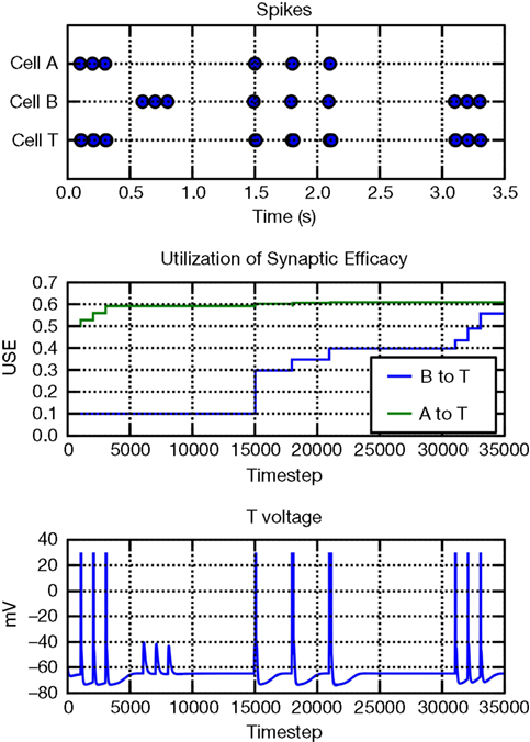
Figure 2. Output of Hebbian learning example from the Section “Usage Example: Hebbian Learning”.
Usage Example: Hebbian Learning
Following is a complete, functional example of Brainlab usage. The results of this Brainlab example are shown graphically in Figure 2
, and referring to the plot while reviewing the explanation below will help to make the example clear. (Note however that to reduce space the code below draws only one of the subgraphs shown in Figure 2
.) This simple example demonstrates positive Hebbian learning: when spikes are initially applied to cell A between time 0 s and 0.5 s, the target cell T spikes because the synaptic connection from A to T is initialized to a strong value. However the initial spikes forced onto B by external stimulus (during time 0.5 s to 1.0 s) do not result in the target cell T spiking, because the B to T synapse is initially weak. During time 1.5 s to 2.5 s, a series of three spikes are forced by external stimulus onto both cell A and B. The spike forced on cell A is sufficient to evoke an output spike on T, as we have already seen. The forced spike on B just before the evoked spike on T causes the B-to-T synapse to strengthen through positive Hebbian learning. In the final phase, from time 3.0 s to 3.5 s, we see that after the synaptic strengthening, forced spikes on B are now alone enough to evoke a spike on T. Here is the script:
Usage Example: Rain Network
In this section, we give an example of how Brainlab is used to create a type of model that our lab has called RAIN (Recurrent Asynchronous Irregular Network). This type of asynchronous, irregularly firing network with persistent activity is similar to the models investigated by Vogels and Abbott (2005) and it is also a benchmark model used in the Brette et al. (2007)
review of neural simulator systems. Our network has 4000 leaky integrate-and-fire neurons, 80% excitatory and 20% inhibitory. Each neuron is defined as a single compartment model with a time constant,  The neuron will generate an action potential and the membrane potential will reset to the clamped resting potential for 5 ms whenever the membrane potential crosses the threshold at −50 mV. The excitatory neurons differ from the inhibitory ones with a depolarization-activated, noninactivating potassium channel (Im current), which is responsible for the adaptation of firing rate of cortical pyramidal cells (Yamada et al., 1998
).
The neuron will generate an action potential and the membrane potential will reset to the clamped resting potential for 5 ms whenever the membrane potential crosses the threshold at −50 mV. The excitatory neurons differ from the inhibitory ones with a depolarization-activated, noninactivating potassium channel (Im current), which is responsible for the adaptation of firing rate of cortical pyramidal cells (Yamada et al., 1998
).Both excitatory and inhibitory type synapses are simulated as conductance changes with instantaneous jump at maximal value and exponential decays, i.e., a presynaptic event generates a synaptic conductance change of  , which decays according to the following equation:
, which decays according to the following equation:
The synaptic time constants are 5 and 10 ms, and quantal conductances are 5 and 50 nS for excitatory and inhibitory synapses, respectively. All synapses are created with synaptic delay chosen from a normal distribution with a mean of 1 ms and standard deviation of 1 ms.
Neurons were randomly connected by a probability of 2% by conductance-based synapses (Gupta et al., 2000
). For outbound inhibitory connections, we incorporate the diversity of GABAergic interneurons. The experiment performed by Gupta et al. (2000)
indicates that GABAergic synapses in neocortical layers II to IV have three statistically distinct types of synapses, where each type has particular temporal dynamics of synaptic transmission. The synapses were modeled according to the concepts of the refractoriness of the release process (Markram et al., 1998
) as shown in Table 1
. The Brainlab code below demonstrates the creation of a new synaptic facilitation and depression profile called
sfd_1 by copying a standard Brainlab library profile called F1. Once copied, the new profile is modified according to data in Table 1
.
Next we create an new inhibitory synapse profile called
InhSyn1 that is based on the Brainlab standard profile called I. The facilitation and depression profile just created is then embedded into the new synapse type. Note that some extraneous parameters inherited from the default profile are also deleted at this time, and note that the reference to the facilitation and depression profile is made to the newly-created variable, rather than the text string name of the profile (though Brainlab supports either, the former is generally easier and less error prone):
We omit the section of Brainlab code that creates the cells themselves, but the procedure is similar: a basic cell type is copied from the Brainlab library and a few parameters are selectively modified. The variables returned from the Brainlab function that creates the cells groups are stored in a Python list. So
e[0] references the first group created, e[1] the second group created, and so on.Brainlab provides a single, general
AddConnect(from, to) method that can make connections at all three connection levels supported by NCS (within-layer, between-layer, and between-column). The modeler does not need to pay attention to NCS’s distinction between these three levels of connection if this is not desired, and this encapsulation can hide much complexity from the user. Furthermore, connections can conveniently be made in Brainlab using the Python variables assigned to the created objects, rather than their underlying .in file text names (which the modeler can basically ignore). In our example of a 4000 neurons network, we do divide the network into five cell groups, so that it could be distributed to five computational nodes. The three types of inhibitory synapses connect to both inhibitory and excitatory neurons in the network:
The short-term dynamics of inhibitory synapses not only maximize the synaptic diversity, but potentially constrain the functional impact of different interneurons on the long-term dynamics which exist among the excitatory neurons. To incorporate this idea into the model, we also include the spike timing dependent plasticity (STDP) within each cell group (Song et al., 2000
). The Brainlab code for these connections is as follows:
Even the fairly simple RAIN network example shown above results in a multi-thousand line
.in file for NCS. The more concise, programmatic representation of the model in Brainlab makes it easier to create and also easier for others to quickly understand the true structure of the model.We have shown elements of the design, implementation, and usage of Brainlab, a Python toolkit that leverages the strengths of Python to provide a more powerful and convenient interface to the NCS network simulator. We integrated Brainlab to NCS loosely, in a way that required no source code changes to NCS whatsoever. We were able to design a Pythonic neural modeling interface that can automatically convert an object representation into NCS’s cumbersome
.in representation. For simulation, we also integrate Brainlab loosely with NCS, using Python’s sub-process management and standard operating system level tools like ssh for remove invocation as necessary.Our approach gives us simplicity of implementation and ease of long-term maintainability, with no significant performance penalties on simulations, yet still extends to NCS all the considerable power and flexibility of Python and its numerical, graphical, special format file access, and other support packages.
Brainlab will likely remain the Python toolkit for NCS, and will see use for those applications where NCS’s own strengths make it the tool of choice: large scale simulations with a medium degree of biological realism.
The authors declare that the research was conducted in the absence of any commercial or financial relationships that could be construed as a potential conflict of interest.
Portions of this work were supported by grants from the U.S. Office of Naval Research (grants N000140010420 and N000140510525).
- ^ http://brain.cse.unr.edu/
- ^ http://brainlab.sourceforge.net/
- ^ http://www.nest-initiative.org/index.php/Main_Page
- ^ http://www.nest-initiative.org/index.php/PyNEST
- ^ http://www.neuron.yale.edu/neuron/
- ^ http://www.genesis-sim.org/GENESIS/
- ^ http://neuralensemble.org/trac/PyNN/
- ^ http://www.neuralensemble.org/
- ^ http://www.lsm.tugraz.at/pcsim/
- ^ http://brian.di.ens.fr/
- ^ http://topographica.org/Home/index.html
- ^ http://matplotlib.sourceforge.net/
- ^ http://pyopengl.sourceforge.net/
- ^ http://numpy.scipy.org/
- ^ http://www.scipy.org/
- ^ http://docs.python.org/extending/
- ^ http://www.openssh.org/
- ^ http://pyopengl.sourceforge.net/
Brette, R., Rudolph, M., Carnevale, T., Hines, M., Beeman, D., Bower, J. M., Diesmann, M., Morrison, A., Goodman, P. H., Harris, F. C., Zirpe, M., Natschläger, T., Pecevski, D., Ermentrout, B., Djurfeldt, M., Lansner, A., Rochel, O., Vieville, T., Muller, E., Davison, A. P., El Boustani, S., and Destexhe, A. (2007). Simulation of networks of spiking neurons: a review of tools and strategies. J. Comput. Neurosci. 23, 349–398.
Drewes, R. (2005a). Brainlab: A Toolkit to Aid in the Design, Simulation, and Analysis of Spiking Neural Networks with the NCS Environment. Master’s Thesis, Reno, University of Nevada. Available at: http://www.interstice.com/drewes/brain/thesis.pdf
Drewes, R. (2005b). Modeling the Brain with NCS and Brainlab. Linux Journal, pp. 58–61. Available at: http://www.linuxjournal.com/article/8038