Mapping transient hyperventilation induced alterations with estimates of the multi-scale dynamics of BOLD signal
1
Department of Diagnostic Radiology, Oulu University Hospital, Oulu, Finland
2
Department of Information and Electrical Engineering, University of Oulu, Oulu, Finland
Temporal blood oxygen level dependent (BOLD) contrast signals in functional MRI during rest may be characterized by power spectral distribution (PSD) trends of the form 1/fα. Trends with 1/f characteristics comprise fractal properties with repeating oscillation patterns in multiple time scales. Estimates of the fractal properties enable the quantification of phenomena that may otherwise be difficult to measure, such as transient, non-linear changes. In this study it was hypothesized that the fractal metrics of 1/f BOLD signal trends can map changes related to dynamic, multi-scale alterations in cerebral blood flow (CBF) after a transient hyperventilation challenge. Twenty-three normal adults were imaged in a resting-state before and after hyperventilation. Different variables (1/f trend constant α, fractal dimension Df, and, Hurst exponent H) characterizing the trends were measured from BOLD signals. The results show that fractal metrics of the BOLD signal follow the fractional Gaussian noise model, even during the dynamic CBF change that follows hyperventilation. The most dominant effect on the fractal metrics was detected in grey matter, in line with previous hyperventilation vaso-reactivity studies. The α was able to differentiate also blood vessels from grey matter changes. Df was most sensitive to grey matter. H correlated with default mode network areas before hyperventilation but this pattern vanished after hyperventilation due to a global increase in H. In the future, resting-state fMRI combined with fractal metrics of the BOLD signal may be used for analyzing multi-scale alterations of cerebral blood flow.
Natural phenomena, from coastline dimensions to organization of brain functional connectivity, incorporate self-similarity; i.e. the proportional characteristics of the observed variables resemble each other in multiple scales (Mandelbrot, 1975
; Maxim et al., 2005
; van den Heuvel et al., 2008
; Wink et al., 2008
). The latin word fractus (engl. broken), was first used by Mandelbrot to describe the whole phenomenon as being based on these repeatable small pieces, as if they were broken parts of the whole (Mandelbrot, 1975
).
Fractal temporal signals have power spectrum characteristics following a 1/f trend (Herman et al., 2009
; Maxim et al., 2005
; Sprott et al., 2003
). Functional magnetic resonance imaging (fMRI) can provide temporal signals reflecting the blood oxygenation level (BOLD) contrast with T2 and T2*-weighted image sequences (Ogawa et al., 1990
). In the absence of cued stimuli, the BOLD signal variations in the brain follow a power spectral distribution (PSD) trend 1/fα, where f is the frequency and α is an index describing the trend (Biswal et al., 1995
; Kiviniemi et al., 2000
, 2005
; Purdon and Weisskoff, 1998
; Zarahn et al., 1997
). In the frequency domain, the parameter α (also often referred to as the spectral index β) describes the PSD trend slope on a logarithmic scale.
Fractal signals fall into two categories, depending on whether they have a stable (fractional Brownian motion, fBm), or a time dependent variance (fractional Gaussian noise, fGn) (Herman et al., 2009
; Maxim et al., 2005
). The Hurst exponent (H) and the fractal dimension (Df) have been used to estimate the scale invariant features of the time series. According to Sprott (2003)
, the H and Df are related to α by equations α = 2H − 1 and α = −2Df + 3 in fGn model. The H is most often used as it can describe the most essential scaling properties of a temporal signal on a scale from 0 to 1. Df on the other hand can be used to describe the high dimensionality of the structure with a scale in theory from 0 to infinitum (in practice from 0 to 3, Herman et al., 2009
).
Theoretically, BOLD signal fluctuations form as an interference of physiological processes affecting the deoxyhemoglobin level in the cortex (Kiviniemi, 2008
). Spontaneous low frequency fluctuations (LFF) affecting the cerebral cortex, i.e. vasomotor, pCO2, electrophysiologic and metabolic fluctuations all affect the detected T2*-weighted signal (Kannurpatti et al., 2008
; Laufs, 2008
; Obrig et al., 2000
; Pattison et al., 2009
; Shmuel and Leopold, 2008
). It has been shown that sedation, blood withdrawal and brain diseases all increase low frequencies of BOLD fluctuations in a wide range and alter 1/f trends (Kannurpatti et al., 2008
; Kiviniemi et al., 2005
; Zang et al., 2007
). Metrics measuring multiscale effects in BOLD signal 1/f trends have high potential for giving crucial information on the dynamics of the brain cortex.
In this study, we aim to find a suitable metric for characterizing dynamic multi-scale changes in cerebral blood flow. We used hyperventilation to induce a transient cerebral blood flow (CBF) reduction. A transient CBF reduction also alters the vasomotor fluctuations dynamically in several temporal scales; i.e. the flow returns towards a normal level within minutes, and the increased vasomotor waves gradually return towards the original level (Kannurpatti et al., 2008
). We hypothesize that differences in metrics measuring the 1/f trends (α, H, Df) could be used to localize the effects of the dynamic CBF alterations in the brain cortex. In the analysis of 1/f fractal properties, the temporal stability of variance, i.e. the fBm or fGn nature of the signal, should be examined and accounted for. Therefore we also investigated whether fBm or fGn model based analysis methods would be more accurately matched with grey matter signal behaviour.
Subjects, Experimental Setup and Imaging Procedure
Twenty-three healthy student volunteers (six females, mean age 25 ± 3 years) were imaged in rest with closed eyes in normal ad liberam ventilation before and after 2 min of hyperventilation. The study was approved by the Ethics Committee of the University of Oulu, and each subject gave written informed consent. The imaging was performed by a 1.5-T General Electric Signa HDX scanner using 8-channel head coil with a parallel imaging acceleration factor of 2. Hearing was protected using earplugs, and motion was minimized using soft pads fitted over the ears. Two separate scanning sessions were performed, one before (Pre-HV) and one after hyperventilation (Post-HV) using GR EPI sequence with 1764 ms TR, 40 ms TE, 90° flip angle, 25.6 cm × 25.6 cm FOV and 64 × 64 image matrix. The whole brain volume was covered using 28 slices, with 0.4 mm space between slices and a 4 mm slice thickness. 250 brain volumes, lasting 7 min 21 s, were collected after exclusion of the first three volumes due to T1 equilibrium effects. In addition to resting-state fMRI, T1-weighted 1 mm3 voxel scans were taken with 3D FSPGR BRAVO-sequence in order to obtain anatomical images for segmenting the brains and for co-registration of the fMRI data to standard space coordinates.
Physiological Measurements and Hyperventilation Procedure
The subjects were monitored with a Schiller Maglife C 400G MRI-compatible anaesthesia monitor. Expiratory end tidal CO2 (ETCO2) was measured from an MRI-dedicated ventilation mask. Peripheral blood oxygen saturation (SpO2) and heart rate (HR) were measured from the right index finger tip. Diastolic (DP) and systolic (SP) blood pressure were measured from the left arm using an automated cuff. The measurements were taken before the first resting-state scans, and during the last 15 s of the hyperventilation periods before the second resting-state scans. DP and SP were successfully collected from 16 subjects; hyperventilation-related motion artefacts prevented the automated measurement of blood pressure in seven subjects prior to the second scan.
During hyperventilation, the subjects were instructed to breathe forcefully as deeply and as quickly as they could for 2 min. The physiological measurements were repeated at the end of hyperventilation just before the start of the second resting state. During each of the scans the subjects breathed spontaneously. One of the authors (VK) gave the instructions, and monitored the subjects beside the scanner throughout the duration of scanning sessions.
To ascertain that hypocapnia was induced by hyperventilation, the group level differences of normal ventilation and hyperventilation-induced state in physiological measurements (ETCO2, SpO2, HR, DP and SP) were evaluated with paired t-test (states Pre and Post respectively; Table 1
). SPSS software version 14.0 was used for the data processing.
Processing of Structural Brain Images
The 3D FSPGR images were co-registered with the fMRI datasets of corresponding subjects and with a Montreal Neurological Institute (MNI) standard structural space template (avg152T1 template included in FSL) to produce transformations for spatial normalization of the fMRI results. FSL 4.0 FLIRT with default settings was used for registrations. The brain was extracted from the 3D FSPGR and BOLD images prior to registrations with the FSL 3.3 BET tool (f = 0.25 and f = 0.5 respectively, g = default).
Grey matter (GM), cerebrospinal fluid (CSF) and white matter (WM) were segmented from the original brain-extracted 3D FSPGR data using the FAST segmentation tool in FSL 4.0 (default settings). The resulting subject-specific probabilistic segment maps were co-registered to MNI-templates with the same transformations as whole-brain structural images.
Registered segments and whole-brain structural images were averaged to produce group level mean segments and anatomy for overlaying the fMRI results on them, and for correlating the fMRI results with them. Whole-brain structural images were intensity-normalized prior to averaging by dividing their intensities with their mean intensity.
fMRI Pre-Processing
Brain extraction was carried out for BOLD images with FSL 3.3 BET using f = 0.5. Motion was corrected using the FSL 3.3 MCFLIRT. All the subjects exhibited less than 1.5 mm motion, and the mean motion of volumes relative to the previous time point was tested to be not statistically significantly different between the scans before and after hyperventilation. As motion affects the BOLD signal (Friston et al., 1996
), and especially its PSD (Maxim et al., 2005
) even after motion correction, the movement-related confounding effects were removed from the BOLD signal time courses according to Friston and co-workers, using motion parameter estimates produced by MCFLIRT, in-house developed Matlab software and FSL 4 fsl_regfilt tool.
Estimation of Variables α, H and Df
All brain BOLD signal time courses were detrended by fitting a + b × t to them (where t is time). 128-point Discrete Fourier Transformations (DFTs) were computed for 123 128-points wide rectangular windowed sections of detrended time courses. Sections were overlapped by 127 points. Rectangular windowing was used in DFT with a spectrogram function in Matlab. As fMRI time courses are real-valued, their amplitude spectra are positively symmetric, and phase spectra are negatively symmetric with respect to Nyquist frequency. Consequently, we only used the first N/2 + 1 coefficients of N-point DFT. As a result, 64 DFT coefficients were obtained for each 128-point section. PSDs were estimated as second powers of amplitude spectra (divided by the number of samples and sampling frequency). The final PSD estimate for a time course was computed by averaging PSDs from individual sections. The averaging reduces noise related to the selection of the sampling period (Ifeachor and Jervis, 2002
), but works under the assumption of at least some stationarity in the signal.
The actual 1/fα PSD trend of individual BOLD time courses were modelled through α by fitting a + b × f−α to their PSD (Kiviniemi et al., 2000
, 2005
). The Ezyfit 3rd party toolbox
1
(version 2.04, default settings) was used for fitting the model to individual PSDs (initial values a = 0, b = 1, α = 0).
For estimation of the Hurst exponent H and fractal dimension Df, both original and integrated versions of the detrended BOLD time courses were used as inputs for the estimation algorithms. The value at each time point in an integrated time course is a sum of the values at corresponding and previous time points in an original, detrended BOLD time course. This way the estimation of H and Df assumes fractional Gaussian model (fGn) of underlying BOLD PSD trends, which has been shown to be a fit description of resting-state BOLD data corrected for motion-related confounding effects (Maxim et al., 2005
). In the fractional Brownian motion (fBm) model analysis, the original BOLD time courses were used as was earlier suggested by Maxim et al. (2005)
.
Three estimates of H were computed from integrated BOLD signals with the Matlab function wfbmesti. One estimate given by this function is based on discrete the second-order derivative (DOSD) method (Istas and Lang, 1994
) and another on the wavelet-based version of DOSD. A third one uses the linear relationship that exists on a double-logarithmic scale between the variance of details produced by wavelet transformation and the corresponding detail level (Flandrin, 1992
). These three estimates are later denoted as HDOSD, HWDOSD and HFWD.
One estimate of Df was calculated from integrated BOLD signals according to Higuchi. This method has been demonstrated to give stable estimates with limited data (Higuchi, 1988
; Klonowski, 2007
), which is also the case regarding the length of BOLD time courses. The procedure involves computing a curve length (line integral) of the original time course and average curve lengths of its down-sampled versions. Down-sampled versions of time courses are used to extract information about signal characteristics on different scales. The curve lengths constitute a line when plotted on a double-logarithmic scale (base 10) against the lengths (k) of corresponding down-sampling intervals. The absolute value of the slope of the line is the fractal dimension.
Individual average curve lengths may be sensitive to outliers. If there is a wave form present on one scale, but not on others (i.e. some deterministic pattern that would yield a spike in the PSD that does not follow the general underlying trend of that PSD), this could bias the line fit in a double-logarithmic coordinate system. In other words, the original algorithm of Higuchi could be sensitive to distinct BOLD fluctuations with large enough amplitude. In order to overcome this problem, we investigated the use of median instead of mean curve lengths on different time scales, since median is more insensitive to individual large outliers. From here on, the values of Df estimated with the original algorithm are denoted by DfH, and the values estimated with the modified algorithm by DfHmedian.
Analysis of BOLD Data Using Variables α, H and Df
The estimation resulted in variables α, HDOSD, HWDOSD, HFWD, DfH and DfHmedian for each voxel for the states of normal (state Pre) and hyperventilation-modulated CBF (state Post). Subject-level brain maps of these values were spatially normalized using transformations obtained from co-registration of 3D FSPGR to the original BOLD data and MNI template (c.f. “Processing of structural brain images”).
After spatial normalization, we tested on the group level whether each variable in each voxel (i.e. MNI standard space coordinate) exhibited a statistically significant change between the states. The testing was done with a T-statistic in a permutation test framework. The randomise tool in the FSL software was used with 10,000 permutations and with threshold-free cluster-enhancement (TFCE) for multiple comparisons correction. TFCE (Smith and Nichols, 2007
) does not require cluster-level thresholds, making the results independent of any bias due to arbitrary cluster-forming threshold selection. Since TFCE enhances areas with values exhibiting spatial contiguity, it should be suitable for use in this study since we expected those values (changes of variables α, H and Df) to be extensively present and quite uniform in GM. Randomise was run separately for positive and negative changes between the states: 1-sample testing was used on Post minus Pre, and Pre minus Post variable values of all patients in each voxel, resulting effectively in 2-sample paired testing.
The resulting group level 1-p maps describing corrected p-values were spatially correlated to probabilistic group level mean tissue segment maps with the FSL 4 fslcc-tool (Table 2
). Confidence intervals (CI) for correlation coefficients were calculated using normality transformation. This shows how sensitively and specifically changes from baseline resting-state values of variables due to altered CBF correspond to GM, and thus how potent these changes are as temporal feature contrasts in detecting changes in CBF. For variables α and H, the correlation was calculated using 1-p maps corresponding to testing of Post minus Pre values, and for Df-variables using 1-p maps corresponding to testing of Pre minus Post values, since these are the dominant directions of change in these variables (Figures 2
–4
).
Physiological variables such as ETCO2, HR and DP changed significantly between the states (p < 0.01; Table 1
), while SpO2 and SP did not. The significant change of ETCO2 agrees with the assumption that an hypocapnic state was achieved with the hyperventilation procedure.
Figure 1
shows mean FFT power spectra of probabilistic segments of the brain cortex. In all of the spectra, the power at the lowest frequencies is elevated, clearly altering the shape of the power spectrum rather than elevating any single frequency. The lowest frequency trends prevail after removing the signal trends suggestive of dynamic changes in BOLD variance throughout the POST-V scan.
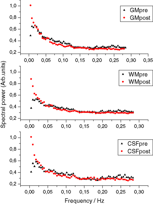
Figure 1. The grey (GM), white (WM) and cerebrospinal fluid (CSF) mean power spectral before (pre in black) and after (post in red) hyperventilation, showing the elevation of the power at the lowest frequencies and the altered PSD configuration after hyperventilation.
Figure 2
illustrates the mean α, H and Df-histograms of the segmented brain voxels. Fractional Brownian motion and Gaussian noise hypotheses were both used to calculate the Df and H metrics. The α-values stay within −1 < α < 1-limits, showing that the variance is not time dependent, and therefore the BOLD signal in both states matches with an fGn model rather than an fBm model. Also regarding the fGn model, Df estimated from integrated BOLD time courses varied between 1 and 2, and H between 0 and 1, as they should. The histograms of fBm measurements both in Df and H show no significant difference between the pre and post-hyperventilation scans, also pointing to the same conclusion. Based on the findings, we chose to use the fGn model in the following estimations of the metrics. The median yields even greater separation between the states in Df measurements.
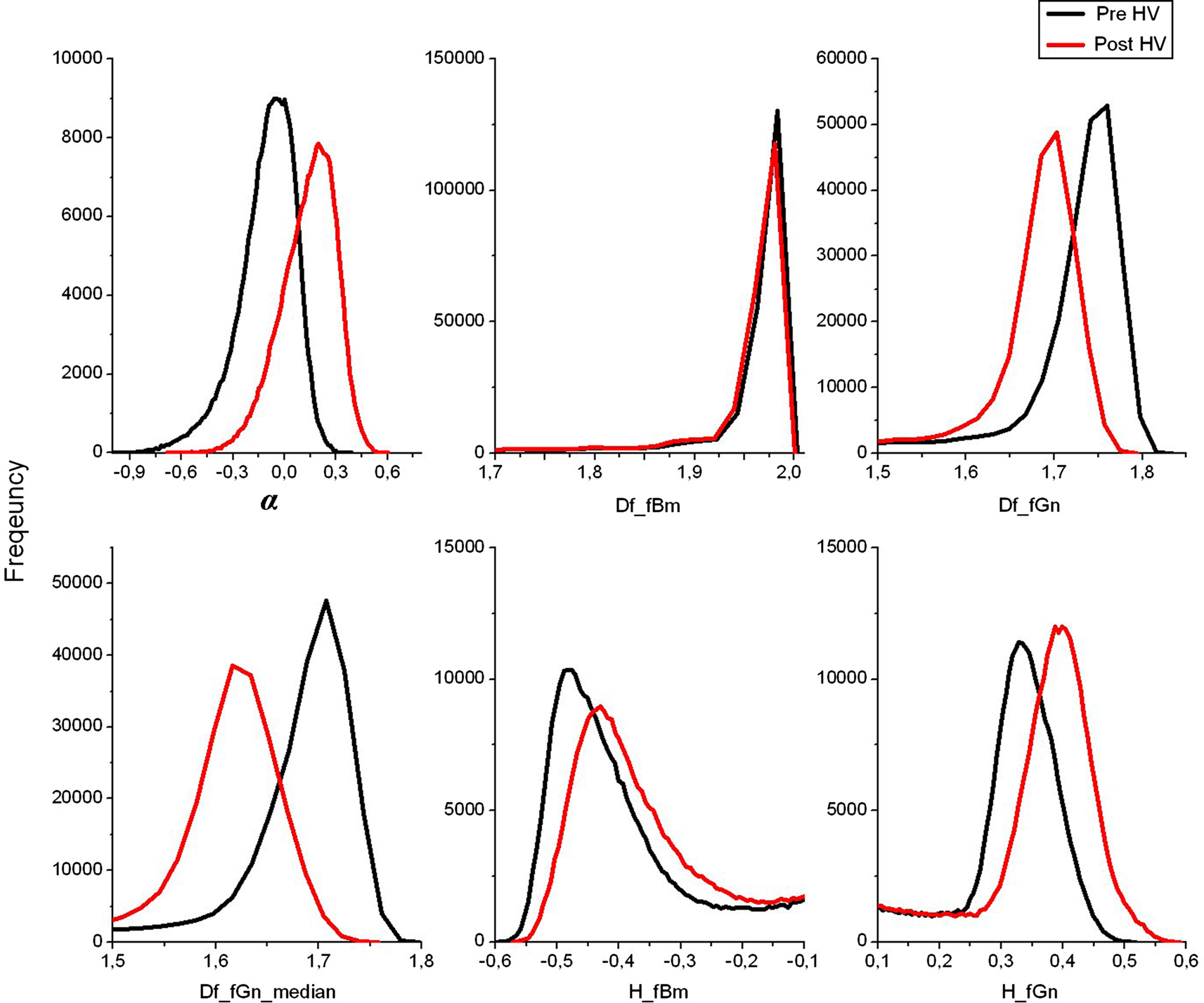
Figure 2. Group mean histograms of α, Df and HFWD of the whole brain. The fBm and fGn model options were both assessed for Df and H.
The mean values of α, H and Df based on the fGn model from mapped probabilistic regions of interest are shown in Table 2
. The changes are in line with the idea that hyperventilation related blood flow reduction transiently increases in low frequency fluctuation. There were significant changes detected between the pre and post-hyperventilation scans in α, HFWD, DfH and DfHmedian in the selected ROI’s. DOSD and wavelet DOSD values were not significantly altered.
The group level mean maps of estimated α showed a significant change in cortical structures between pre and post-hyperventilation scans (Figure 3
). Please note that in the normal status, the cerebral blood vessel-related pulsation of the major cerebral arteries dominate the α values with the given threshold. After hyperventilation, the arterial pulsation dynamics completely alter and a low frequency fluctuation in the cortex becomes a dominant source of the α contrasted map.
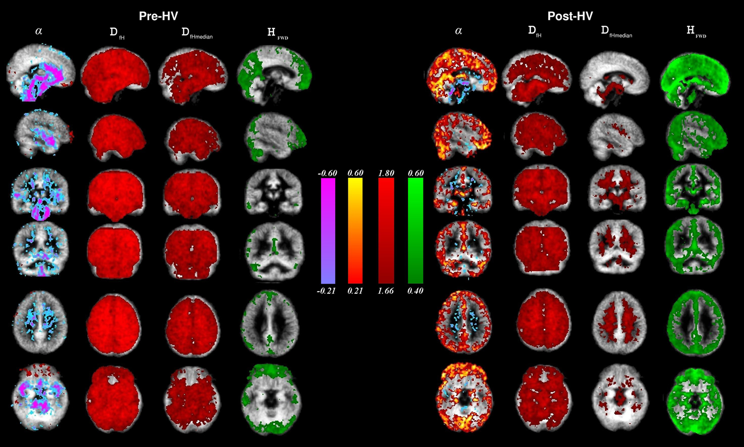
Figure 3. Group mean images α (hot-cold), DfH, and DfHmeadian (red) and HFWD (green) in the brain during the state of normal ventilation (Pre-HV, on the left) and after hyperventilation (Post-HV, on the right) were overlaid on an MNI-coordinated grey matter template image. The range of color-encoding of each metric is shown in the middle of the image.
Unlike the α plots, the Df values are quite uniform over the whole brain in normal ventilation (Pre-HV), c.f. Figure 3
. The fractal dimension, in contrast to both α and H, is reduced during reduced blood flow in the brain cortex after hyperventilation, as predicted. The DfHmedian version of the Df analysis is more sensitive to grey matter changes than the version using mean DfH, c.f. Figure 3
. This is in line with the histogram results in the Figure 2
, showing more differentiation between the two conditions.
Interestingly, the H presented focusing on the ventromedial frontal, parieto-occipital and precuneal cortices similar to default mode regions, as well as visual cortices in occipital lobe (Fox and Raichle, 2007
). Also the HFWD analysis was highly sensitive to differences in the BOLD signal between pre and post-hyperventilation scans; following hyperventilation the H increased throughout the cortex and the default mode-pattern vanished with the given thresholding, c.f. Figure 3
.
Table 3
shows how well 1-p maps describing the significance of variable changes between states (Pre and Post), spatially correlated with GM, CSF and WM. There was a strong anatomical similarity between a change of all variables (α, H, Df), although DOSD-method based estimates of H performed poorly in every way. The confidence intervals in the r-values are very small relative to the differences between the r-values with the ∼2.9 × 10⁵ voxels in the analysed ROI. Therefore all the differences between the r-values are significant in Table 3
. Quantitatively, variables α, DfH, DfHmeadian and HFWD provide quite similar accuracy for mapping the effects of CBF change within the brain cortex. However, some qualitative differences in the spatial distribution of the detected alterations do exist.
Figure 4
shows statistically significant (p < 0.05, TFCE corrected) changes of variables α, HFWD, DfH and DfHmedian overlaid on the probabilistic GM segment. In line with the quantitative measure of spatial correlation of probabilistic segment maps of GM, WM and CSF (Table 2
), the most significant changes of variables were detected in GM, in agreement with the BOLD signal origin. Concerning sensitivity to GM, the change of DfHmedian provided the contrast best coinciding with it. α provided the second best contrast in this sense, while HFWD and DfH had performances similar to each other. However, sagittal views revealed that, in general, no variable changed significantly in the occipital cortex around the visual cortex or at susceptibility artefact areas near the mastoid and frontal sinuses.
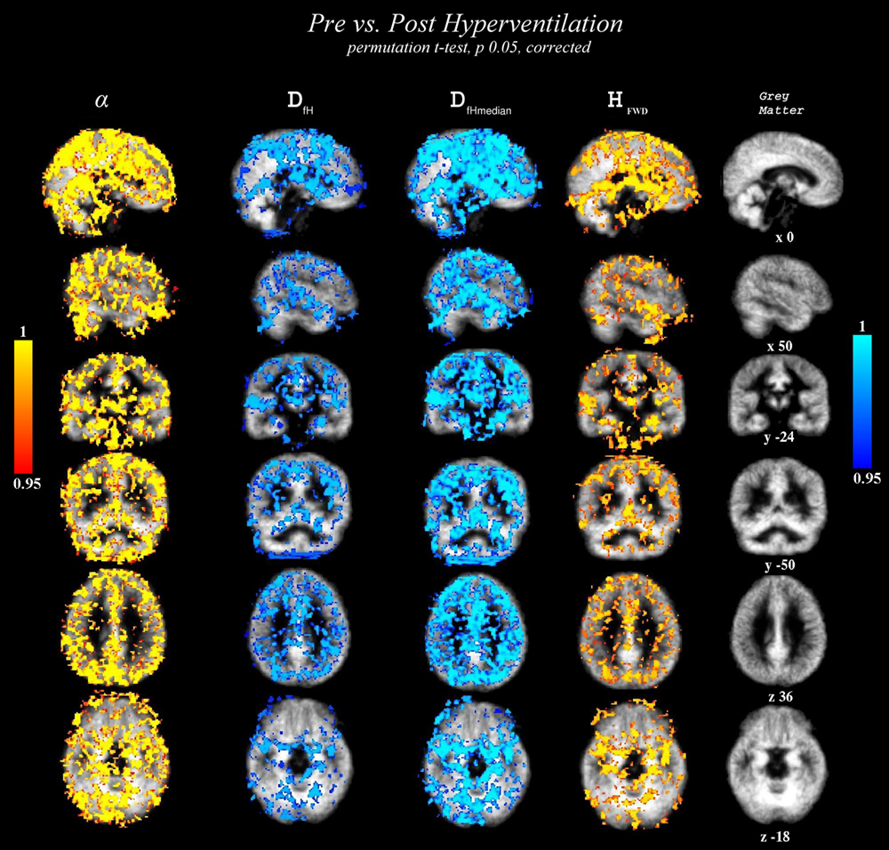
Figure 4. Statistically significant variable changes (between the state of normal ventilation (Pre) and the hyperventilation modulated state (Post) (2-sample paired TFCE corrected permutation test, p < 0.05). The detected voxels are overlaid on the group level mean GM segment in the MNI coordinates in the same locations as in Figure 3
. From left to right: α, DfH, DfHmedian and HFWD. Cold-blue colours = decrease, and warm red-yellow colours = increase in variable between Pre and Post, respectively.
According to the sagittal view in Figure 4
, there is a lack of significant change in the metrics in the visual cortex, precuneus, temporal cortex. Changes in the superior temporal areas in DfH, DfHmedian and HFWD are not detected as clearly as in α. These results indicate that changes of variables are not uniform throughout the cortex. Accordingly, the spatial correlation results (Table 3
) remain clearly below the identical correlation of 1. Interestingly, the BOLD signal trends alter significantly along major blood vessel structures, also suggesting vasomotor changes. Also a spot in the bilateral hippocampi was noticeable in all the measures, but it was not uniform through the limbic regions.
In this study, BOLD signal power spectrum estimates α, H and Df were found to alter significantly between scans taken before and immediately after 2 min of hyperventilation. Quantitatively, all variables have a similar performance in terms of the goal of mapping these effects. The spatial correlation of the detected changes was highest with the grey matter maps of the same group, suggesting that areas responsive to respiratory challenges are dominantly located in those cortical structures with the highest CBF.
As the cardiorespiratory challenge that we used was a dynamic change occurring over several minutes after cessation of hyperventilation, (i.e. while the pCO2-level was normalizing), it was hypothesized that the variance of the BOLD signal might alter as a function of time, i.e. be fBm in nature. However, after spin history and motion correction, the BOLD signal behaves according to the fGn rather than the fBm theory based on the −1 < α < 1 type histograms (Maxim et al., 2005
). This means that the variance of the BOLD signal does not change as a function of time, and the fGn analysis option is valid also in this study. The subsequent analyses of both Df and H were therefore performed according to the fGn hypothesis.
Despite the slowly returning arterial CO2-level and the subsequent diminishing of low-frequency vasomotor effects after hyperventilation, the changes of BOLD signal characteristics were successfully observed in the cortical structures. Furthermore, the changes of variables α, H and Df observed in this study were found to be located in the same cortical structures as block design respiratory tests have shown vasoreactivity and arterial blood flow reserve alterations (Hedera et al., 1996
; Lu et al., 2003
; Lythgoe et al., 1999
; Rostrup et al., 1994
; van der Zande et al., 2005
; Vesely et al., 2001
). Hyperventilation has also been shown to reduce electrophysiological complexity brain cortex and vagal outflow. (Müller et al., 2003
; Penttilä et al., 2003
).
Through similar map assessment, contrast based on DfHmedian was also found to least coincide with the CSF segment at the cortical boundary, making it more specific to GM than the contrast based on straight-forward PSD trend estimation (contrast based on α). Considering some coincidence observed between changes of all variables and the WM segment, we argue that it is probably due to partial volume effects in image data collection causing some GM to contribute in areas mainly occupied by WM. Also the interindividual anatomical variability across subjects affects the results, dispite spatial normalization.
The property of α maps to be able to differentiate between blood vessels and cortical structures makes it a very informative tool in the overall assessment of BOLD signal dynamics. The resting-state map of α in the state of normal ventilation (state Pre, Figure 2
) also corresponded to the earlier results (Maxim et al., 2005
).
HFWD was the only Hurst exponent estimate evaluated in this study that provided reasonable results in mapping the effects of CBF alterations. A more detailed study of the signal properties would be required in order to understand which factors led to the insensitive H estimate when using DOSD-based methods. Different applications are likely to require different choices of estimators; for example, in Maxim et al. (2005)
H was used in the analysis of Alzheimer’s disease by measuring the aspects of fGn noise that may reflect the BOLD response related more on the neuronal activity. Maps of regional homogeneity (ReHo) and amplitude of low frequency fluctuation (ALFF) tend to give rather similar maps (Zang et al., 2004
, 2007
) focusing on default mode areas (Fox and Raichle, 2007
). This pattern was abolished after hyperventilation, as the H increased over the whole cortex. This effect may be confounded by attentional shifts in the default mode after the rather demanding hyperventilation challenge.
As maps and ROI based analysis of the most significant variable changes were inspected (Figure 3
; Table 2
), changes of the fractal dimension estimate DfHmedian provided the contrast that coincided best with GM, and consequently also with changes in BOLD signal generation from physiological processes related to CBF. The alteration of the blood CO2 level due to hypocapnia induces a global reduction of blood flow, and its effects can be prominently detected in grey matter and CSF, less so in white matter (van der Zande et al., 2005
). Occipital areas of GM (sagittal view) failed to be mapped with a change of any variables. The vasomotor reactivity may not be so prominent in these areas due to the reduced number of sympathetic nerves controlling the posterior cerebral artery compared to other parts of the brain (Heistad, 1984
).
The estimation of α was based on averaged spectral estimates of segments that were computed without zero-padding regarding DFT. This also makes the estimation of α itself more stable. The estimation could, however, be regionally biased toward some direction or another, if the temporal BOLD signal in those areas contains signal components with high power on some characteristic frequencies, thus affecting the PSD fitting procedure used to acquire α. With current knowledge of characteristic resting-state BOLD signal PSD spikes, i.e. the prominent frequencies, it would be challenging to filter these effects automatically from the signals, without affecting the baseline signal and, consequently, the estimation of α.
The estimation used for Df is suitable for data analysis with relatively few time points (Accardo et al., 1997
; Higuchi, 1990
). Accardo et al. (1997)
showed that less than 125 data points are needed in order to obtain reliable estimations of Df. We have tested the algorithm with 50–500 time points, and agree that stable results can be obtained with at least 150 time points.
In contrast to previous vasoreactivity studies using often hypercapnic elevations of pCO2 with repeated blocks of respiratory challenges, there were no respiratory nor other challenges going on during the scanning. A 2-min respiratory challenge was performed prior to scanning. This was done in order to introduce a dynamic multi-scale CBF alteration without affecting or stimulating the subject during scanning. The transient hypocapnia returns to normal and induces a long time scale change in vasomotor waves and/or CO2-fluctuations (Kannurpatti et al., 2008
; Pattison et al., 2009
). This dynamic low frequency alteration was used, instead of a temporally sustained elevation in the mean BOLD signal intensity level, to give functional contrast to brain structures. The lack of tasks during imaging ensured that there was no interference from task-related neural activity to the resting-state BOLD signals measured. At the same time, confounding hyperventilation related motion artefacts were also minimized.
The hypocapnic state was efficiently achieved based on ETCO2 reduction, although it has to be mentioned that only intubation would give accurate, non-leaked ETCO2-values. Intubation that requires sedation of the awake control subjects was not used for ethical reasons. The expiratory and arterial ETCO2 is closely matched in a supine position, with a difference of 0.8 mmHg (Serrador et al., 2006
). Based on the literature, the ETCO2 reduction of 2.2 kPa (i.e. 16.5 mmHg) achieved in this study will, on average, reduce regional blood flow by 40% and volume by 8% (Last et al., 2007
; Poppel et al., 2007
). Hyperventilation was selected as the method since it has a relatively smaller effect on the cerebral blood volume (CBV) compared to CBF, and thus partial volume effects affecting the BOLD signal caused by changes in blood vessel diameter are minimized (Fortune et al., 1995
).
Despite the dominantly blood flow instead of volume change following hyperventilation, a reduction of 3.6–4.8 ml in brain volume is to be expected, based on existing literature. This grey matter volume loss that will be compensated with CSF space can be estimated. The simultaneous detection of changes in the CSF, WM and GM areas with the BOLD technique may partially result from compensatory volume alterations and subsequent partial volume effects. The same effect is bound to happen also in the more often used studies assessing vascular reactivity with repeated hyperventilation challenges.
A potential application of functional 1/f trend based estimates such as α, H and Df could be the detection of altered vasoreactivity, i.e. vasomotion, in the pre-capillary arteries and the following vessels. Blood perfusion heterogeneity has been shown to be increased during ischemia (Simonsen et al., 2002
). Stroke, transient ischemic attacks or other factors reducing regional perfusion increase the low-frequency vasomotion amplitude and reduce the dominant frequency (Hudetz et al., 1995
; Liu et al., 2007
). A lack of endothelium in tumor neovasculature induces extended hypoxic states that are also reflected in a BOLD signal as low-frequency events altering the temporal signal properties (Baudelet et al., 2006
; Wardlaw et al., 2008
). These metrics may reveal new pathological mechanisms and enable the detection of areas at risk of cerebrovascular incidents.
We agree with Liu et al. (2007) and Baudelet et al. (2006)
that the analysis of the low-frequency characteristics of the BOLD signal offers a new contrast mechanism reflecting changes in vascular physiology in addition to neuronal changes. Indeed recently, the valuation of the microvascular state of rectal tumors have shown promising results (Wardlaw et al., 2008
). As some of the changes in physiological low-frequency factors tend to occur over a wide range of low frequencies, instead of one single frequency, variables related to PSD trends and other features extracted from a temporal BOLD signal could be used as an improved marker of neurovascular integrity in tissue.
As the formation of the BOLD signal is a sum of several oscillations affecting the deoxyhemoglobin, the resulting BOLD signal can be quite complex (Kiviniemi, 2008
). A very important paper addresses this issue by incorporating the method to distinct monofractal and multifractal dynamics (Wink et al., 2008
). This method may improve the sensitivity of the fractal properties, as the stationarity of the fractality is assessed. Also importantly, as the BOLD signal in the brain is an indirect measure of regional neuronal activity, the Hurst exponent type measurement may reveal important information about the long-lasting memory of neuronal population activity over multiple time-scales. The multi-fractality has been shown to be connected to Alzheimer’s disease and medication effects (Wink et al., 2008
).
In general, the factors altering the PSD trend measures α, H and Df need not be solely related to factors affecting CBF. In theory, the assessment of any factor capable of changing the low frequency BOLD signal oscillations (i.e. neuronal or metabolic activity as well) may be detectable as long as CBF, blood pressure and other factors contributing to the oscillations are within normal limits and remain stationary enough during experimentation. At present, it seems that during normal awake status, the neuronal activity fluctuations are a major source of BOLD signal low-frequency fluctuations (Fox and Raichle, 2007
). The fractal dimension estimations described in this study offer new methods that are also applicable in the analysis of neuronal activity reflected in temporal BOLD signals.
Estimates of 1/f trends of temporal BOLD signals can be used in mapping the dynamic multi-scale effects of cerebral blood flow induced by transient hypocapnia in the brain cortex. Estimation of a trend from the PSD itself (estimate α) was able to separate the brain cortex and cerebral arteries. The median variate of a fractal dimension (DfHmedian) estimate may provide a contrast that is more sensitive to changes of vasoreactivity than the Hurst exponent or α. The HFWD was able to detect a default mode pattern during normal status with specific windowing. However, in general, performance of α, DfHmedian and HFWD was rather similar with respect to grey matter specificity in depicting the dynamic neurovascular change. Applications of the metrics could include new diagnostic approaches to disorders affecting cerebral blood flow dynamics and to the assessment of the effectiveness of the treatment of such disorders.
This study was conducted in the absence of any commercial or financial conflicts of interest.
Grants #111711 and #123772 from the Finnish Academy, the Finnish Medical Foundation, and the Finnish Neurological Foundation contributed significantly to the study.
Herman, P., Kocsis, L., and Eke, A. (2009). Fractal characterization of dynamic signals: application to cerebrovascular hemodynamics. In Dynamic Brain Imaging: Mutlimodal Methods and In Vivo Applications, F. Hyder and J. M. Walker, eds (New York, NY, Humana Press, Springer Science + Business Media), pp. 23–42, doi: 10.1007/978-1-59745-543-5.
Pattison, K. T. S., Mitsis, G. D., Harvey, A. K., Jbabdi, S., Dirckx, S., Mayhew, S. D., Rogers, R., Tracey, I., and Wise, R. G. (2009). Determination of the human brainstem respiratory control network and it’s cortical connections in vivo using functional and structural imaging. Neuroimage 44, 295–305.