Detailed understanding of cerebrovascular oxygen transport mechanisms is particularly relevant to popular brain imaging methods that rely on hemodynamics to infer brain activity, such as functional magnetic resonance imaging (fMRI). Generally, such methods use the positive portion of the blood oxygen-level dependent (BOLD) response, which reaches its peak several seconds after a brief period of neural activation. However, there is also interest in the earlier phase of the hemodynamic response. In this period, during the first few seconds after brief activation, there is evidence for a transient drop in intravascular oxygen concentration (
Malonek et al., 1997
;
Vanzetta and Grinvald, 1999
). Moreover, measurements of tissue oxygen concentration clearly show the early deoxygenation, subsequent overshoot, and oscillatory late-time behavior (
Thompson et al., 2003
,
2005
). Here, we provide a model that explains the full time course of these transient changes in tissue oxygen concentration.
These detailed mechanisms of microvascular oxygen transport underlie the BOLD response observed using T2*-weighted magnetic resonance imaging. The time course of the detected contrast changes are, in fact, critically related to changes in intravascular oxygen concentration. An understanding of oxygen transport is a critical requirement, although a complete treatment of the BOLD response naturally involves other factors, such as the signal component associated with extravascular volume changes.
Most attempts to model cerebrovascular oxygen transport have taken rate-equation approaches, e.g., (
Buxton and Frank, 1997
;
Buxton et al., 1998
;
Hayashi et al., 2003
;
Herman et al., 2006
;
Hudetz, 1999
;
Hyder et al., 1998
;
Mintun et al., 2001
;
Zheng et al., 2005
). These models generally combine a non-linear flow model with diffusion in a compartmental geometry. One popular form of flow model is the “windkessel,” a linear lumped-element equivalent system. The classic windkessel consists of two resistors, which represent frictional (viscous) losses, and a compliance, which represents mechanical storage of energy in the elasticity of the vessel walls. This windkessel model is often modified to include a time-varying (“delayed”) compliance to describe the frequently observed “late undershoot” (
Buxton et al., 1998
;
Mandeville et al., 1999
;
Zheng et al., 2002
). Most recently, a few models have offered a combination of convection-diffusion dynamics with such non-linear windkessel flow models in a single-compartment (
Valabregue et al., 2003
) or multi-compartment geometry (
Huppert et al., 2007
).
Here, we offer a simple alternative model that accounts for full time-course of the hemodynamic response, including commonly observed late-time dynamics such as the undershoot. The model treats oxygen transport as a diffusive process that is distributed throughout the arteriolar tree. This feature is motivated by two key experimental observations. First, oxygen transport in almost all tissues, including the brain, is not limited to capillaries, but occurs throughout the arteriolar tree; see (
Tsai et al., 2003
) for a review. Consequently, the hemodynamic response is likely affected by the distributed diffusion of oxygen from both the arteriolar tree as well as capillaries. Second, endovascular castings (
Harrison et al., 2002
;
Rodriguez-Baeza et al., 1998
) suggest that microvascular control structures are located quite remotely from the gray-matter capillary parenchyma. The castings show the presence of smooth-muscle fibers, the most widely accepted mediator of mechanical blood flow control, only on arteries and larger arterioles, including the penetrating arterioles that enter cortex.
The model’s most novel feature is the inclusion of the inertial effects of moving arterial blood. As the vascular system transitions from small arteries to penetrating arterioles at the pial surface, blood flow makes a transition from inertial to viscous flow as vessel diameters and flow velocities decrease. The Reynolds number,
R =
UD/
n, describes this transition, where
U is the flow velocity,
D is the vessel diameter, and
n is the kinematic viscosity.
R is the ratio of dynamic pressure, a measure of inertial energy content, to shearing stress, a measure of frictional energy loss. Generally, larger cerebral arteries have
R > 1, while arterioles have
R < 1. In fact, small arteries at the pial surface have
R ∼1. For example, if we consider a vessel with
D = 0.2 mm transporting blood with
U = 20 mm/s (
Kobari et al., 1987
), and take
n = 4 centistokes (mm
2/s), we obtain
R = 1. If the transients of the hemodynamic response extend into these relatively upstream regions with similar flow velocities and diameters, they will be accompanied by inertial effects that have been neglected in previous models.
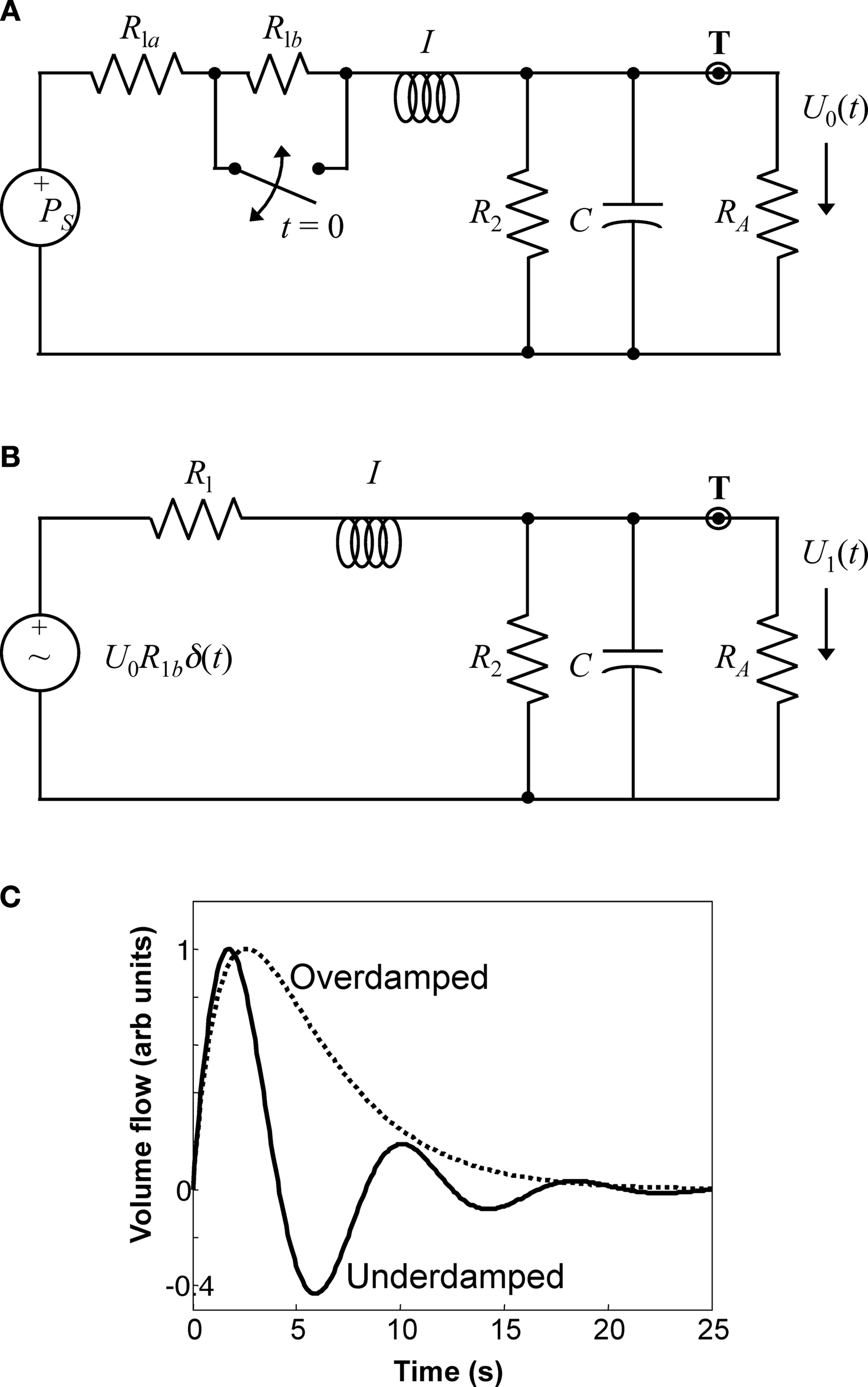
A critical feature of the new work is a simple linear flow model that includes inertial effects, the four-element windkessel (FEW, Figure
1
). The FEW model includes an inertive element, which represents the dynamics of flowing blood, together with the usual compliant and resistive elements, which represent the elasticity of the venous system and frictional losses, respectively. In response to brief neural stimulation in cerebral cortex, we postulate that a correspondingly brief vasodilation in the larger pial vessels gives rise to pressure fluctuations that couple directly to the smaller arterioles, producing corresponding flow velocity perturbations. The FEW model allows blood flow to increase and decrease multiple times in response to a single brief perturbation, an effect analogous to the “sloshing” observed when an elastic container of fluid is sharply disturbed.
Figure 1. The FEW flow model. (A) Lumped-element equivalent circuit schematic. Coupling to the “test” arteriole at T is represented by the load RA >> R2, R1; the steady state pressure at T gives rise to flow U0. At t = 0, a brief upstream vasodilation is represented by the closing of the switch around R1b. The inertive element maintains flow continuity by introducing a pressure transient shown as an impulsive source in (B), which then couples to the load to create flow perturbation U1. (C) Typical examples of underdamped and overdamped flow perturbation impulse responses.
We note that the FEW model is a substantial simplification of the complex flow dynamics associated with the whole of the cerebrovasculature. However, within the context of linear network models, this kind of analogy has been utilized extensively to solve many problems. Complex networks of linear mechanical or fluid elements can always be converted to a Norton or Thevenin equivalent with a multi-pole admittance or impedance (
Olson, 1943
), and this approach has been utilized extensively in cardiovascular applications (
Burattini and Di Salvia, 2007
;
Stergiopulos et al., 1999
;
Thiry and Roberge, 1976
). In this case, we have utilized a second-degree, two-pole model for the impedance transfer function.
As a first step in examining the effects of such inertial dynamics on cerebral oxygen transport, we combine the FEW flow model with a simple one-dimensional, three-compartment, convection-diffusion model for oxygen transport in order to explain measurements of tissue oxygen dynamics during visual cortex stimulation experiments. This combination of the FEW flow perturbations with convection-diffusion dynamics produces a simple but powerful model capable of explaining a wide range of experimental tissue oxygen time-course measurements in mechanistic terms.
Model
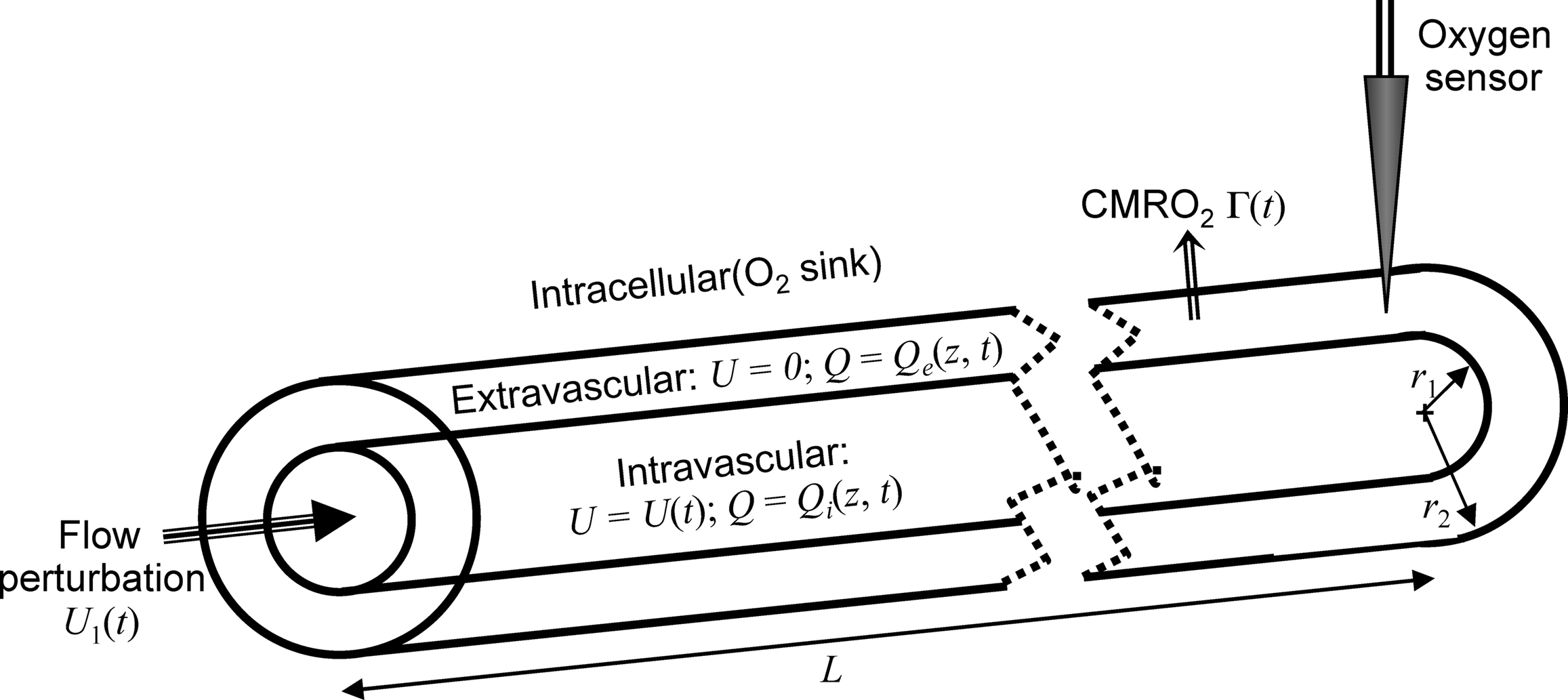
We utilize a simple model geometry, a pair of uniform cylinders of length
L that divides space into intravascular, extravascular, and intracellular compartments (Figure
2
). Although this geometry cannot fully approximate the complex cerebrovascular architecture, it serves as an elementary starting point, roughly representing the aggregate dynamics of the vascular tree from arterioles through the capillaries.
Figure 2. Geometry of the oxygen transport model, showing the intravascular, extravascular and intracellular compartments and their associated description variables for oxygen concentration and fluid flow velocities. The model postulates that an upstream pressure transient drives a flow perturbation at the proximal end of the cylinder, and a sensor samples the oxygen concentration variations near the distal end of the cylinder.
The walls of the inner cylinder permit diffusive transfer of oxygen from the intravascular to the extravascular compartment. In steady-state equilibrium, we assume constant flow of blood inside the cylinder (U0), creating a linear oxygen concentration gradient along its length; the oxygen concentration is higher in the intravascular compartment so that oxygen diffusion matches the uptake of oxygen by the extravascular tissue (Γ0, steady-state CMRO2); the intracellular compartment serves purely as an oxygen sink. Note that this one-dimensional model has no explicit radial variation. Both inner compartments have radially uniform oxygen concentrations with a jump discontinuity between them that drives the diffusive oxygen transfer. In the interest of simplicity we will neglect the non-linear relationship between oxygen concentration in the blood plasma and the erythrocytes. This assumption may distort details of the intravascular modeling, but should permit investigation of the convection-diffusion dynamics on the extravascular oxygen concentration.
At the proximal end of this cylinder we postulate a connection to the larger vascular network in which vasodilation (or other regulatory transient) produces a pressure fluctuation that we can model using the FEW. This linear model allows exchange between the kinetic energy of the blood flow, and the stored energy corresponding to small elastic distortions of vessel walls within the downstream venous compartment, damped oscillatory behavior often called “ringing.” These upstream pressure fluctuations couple directly to flow perturbations, U1(t), within the model intravascular compartment.
In addition to the flow perturbation, we also assume that neural stimulation produces a prompt rectangle-function increase in cerebral oxygen consumption (CMRO2) throughout the extravascular compartment (Γ1). So long as the stimulation duration is short compared to the time scale of the hemodynamic response, this step-function serves as a good approximation, even though the precise time course of the oxygen consumption may be more complex. In modeling results for a few cells, we confirmed that there was no significant difference between the rectangle-function assumption and a time-course that more precisely follows the local neuronal response.
Finally, we assume that a sensor at the distal end of the cylinder measures the effects of these perturbations in the extravascular compartment. Because this sensor measures the oxygen concentration produced by many local capillaries within the gray matter parenchyma, we average the distal portion of model oxygen concentration spatial profile over a length of a capillary segment, ∼60 μm (
Cassot et al., 2006
). Altogether, the model utilizes a total of ten parameters, five of which are generally fixed when the model is applied to fit experimental measurements. Thus, we present a five-parameter model capable of fitting a large experimental dataset.
In the interests of simplicity, we assume that oxygen concentrations are radially uniform and variation only occurs along the longitudinal (z) axis of the cylinder. Thus, the fluid has oxygen concentration Qi(z, t) in the intravascular compartment (r < r1), and Qe(z, t) in the extravascular compartment (r2 > r > r1); the jump discontinuity between these compartments drives the diffusive coupling. We will also neglect longitudinal diffusion in both compartments, a reasonable assumption because longitudinal oxygen concentration gradients will be small compared to the near-discontinuity across the vessel wall. The intravascular fluid has a spatially uniform but time-varying flow velocity, U(t).
Consider a small (differential) length element of the cylinder. In each length element, the change in intravascular oxygen concentration is a balance between the downstream flow of oxygenated blood, and the radial diffusion of oxygen across the vessel wall. The diffusion rate is specified by coefficient A, which is the diffusion conductance weighted by the surface-to-volume ratio of the intravascular compartment (see Appendix for details). A coupled pair of convection-diffusion equations then specifies the relationship between Qi and Qe in this simple system:
where Γ(t) represents oxygen uptake from the tissue (CMRO2).
We will use steady-state equilibrium conditions to specify
A, so we need only specify the differential volume ratios between the compartments,

and β = α/CBV. In steady state, with constant flow
U0 and oxygen uptake Γ
0, this system has a simple linear solution:
We use the steady-state solution to obtain relationships between certain parameters of the model. The model is normalized to the intravascular oxygen concentration at the control point, so that Qi0(0) = 1, and oxygen concentration becomes a dimensionless quantity; this choice gives Γ and A units of inverse time. The oxygen-extraction fraction, E, is specified as the relative oxygen concentration at the downstream end of the intravascular compartment, z = L, so that Qi0(L) = 1 − E, and Γ0 = αEU0/βL. We can then specify the radial oxygen diffusion by choosing the initial relative tissue-oxygen concentration, Qe0(0) = Qe00, so that A = EU0/L(1−Qe00). Thus, specifying α, β, E, U0, L, and Qe00 sets the initial state of the system.
We simulate the experimental response in this system by assuming an initial constant-flow equilibrium, and introduce perturbations in flow, U(t) = U0 + U1(t), and oxygen uptake rate, Γ(t) = Γ0 + Γ1(t). Equation 1 could then be linearized to first order in these perturbations, but we will use the full dynamics to properly model its non-linearities.
We model the flow perturbation using a four-element windkessel (FEW), a lumped linear equivalent-circuit model for the blood flow dynamics (Figures
1
A,B). The inertive element,
I, models Newton’s law regarding the flow of blood in the pial arteries. The series resistance,
R1 =
R1a +
R1b, represents frictional losses associated with the parallel combination of all downstream flow through the fractal vascular tree. The combination of the compliant element,
C, and its parallel resistance
R2, represent the lossy compliance of the downstream venous vasculature. In steady state, and neglecting cardiac pulsatility, there is a constant pressure at point
T, which represents the input to our model three-compartment geometry (Figure
1
A). The model cylinder couples resistively to the larger network, but the load resistance
RA i s much greater than
R1 and
R2, so it does not perturb the global dynamics. The transient behavior of this system is modeled by the switch across
R1b, which briefly closes to simulate a vasodilation that decreases the upstream vascular resistance. Because there was steady-state flow through
I, the vasodilation creates a brief positive pressure fluctuation at
T, which corresponds to the impulse response of the network in Figure
1
B.
Because this system is linear, we need only derive its impulse response function to fully characterize its behavior. The flow perturbation impulse response has three forms depending upon the time constants of the system:
where the first form is under-damped, the second critically damped, and the third over-damped (Figure
1
C). Thus, the flow perturbation is specified by the three parameters:
f, τ, and amplitude
U10. All of the experimental fits utilized flow perturbations that varied from under-damped to critically-damped; overdamped response fits were not observed.
Simulations of Experimental Measurements
We applied the model to a large dataset of oxygen measurements obtained in cat brain area 17 (
Thompson et al., 2003
). In those experiments, visual stimuli were full-field drifting gratings presented monocularly for 4-s periods. During a series of penetrations in three cat brains, combined neuronal and oxygen measurements were collected for a 40-s period starting 10 s before the stimulus onset. Recordings were collected for eight stimulus conditions: seven grating orientations, including the “preferred” (largest evoked spiking orientation, presented to the dominant eye), and only the preferred orientation presented to the non-dominant eye.
We modeled this experiment with two perturbations. First, to model a step-like increase in CMRO
2 during the stimulus period, we set Γ
1(
t) = Γ
10H(
t/
T − 0.5), where H(
t) is the rectangle function and
T = 4 s is the stimulus duration. Second, to model the flow perturbation produced by a step-like dilation of a sphincter control point, we set
U1(
t) =
U1,FEW*H(
t/
T − 0.5), where the “*” symbol denotes convolution. During the fitting procedure, the flow was limited to be ≥0 to avoid flow reversals. Although flow reversals have been observed in individual capillaries, they were not a dominant feature, nor were they observed in larger vessels (
Kleinfeld et al., 1998
). Because our model lumps together the aggregate effects of a portion of the arteriolar tree and capillaries, we consider it reasonable to neglect the effects of flow reversals on the oxygen transport.
We obtained the temporal evolution of the system of Eq. 1 from its initial linear equilibrium by numerical integration using a standard leapfrog technique. The absolute O2 concentration was limited to be ≥0 in both compartments. The two-compartment system was gridded longitudinally into at least 40 steps between 0 and L; more steps were used if needed to enforce a minimum step size of 20 μm. Stability was ensured by making the temporal increment small compared to the steady-state convection, Δt = 0.2 Δz/U0. Stability was assured by running lengthy simulations (e.g., 1000 s) and noting that the equilibrium state persisted with negligible numerical noise when unperturbed, and returned to the equilibrium state after perturbation effects subsided. To improve speed, the numerical integration was coded in C, and then linked to Matlab (Mathworks Corp., Natick, MA, USA). To compare the model to the experimental measurements, the temporal evolution of the relative perturbation of Qe was followed from t = 0–25 s, and the results were sampled over a 60-μm region about z = L.
The full model presented above involves a total of 10 parameters:
E,
U0,
L,
Qe00, Γ
10,
U10,
f, τ, α, and β. We simplified matters by fixing the first three parameters based on experimental observations in the literature. We set the oxygen-extraction fraction
E to 0.44 (
Ito et al., 2004
;
Tsai et al., 2003
;
Vovenko, 1999
), the steady-state flow velocity
U0 to 0.77 mm/s (
Kleinfeld et al., 1998
), and
Qe00 to 0.66 (
Tsai et al., 1998
,
2003
).
The choice of an appropriate value for α requires consideration of gray matter cytoarchitecture. The blood volume fraction in the cortex (CBV) is close to 0.06 (
Ladurner et al., 1976
;
Phelps et al., 1979
). If the oxygen probe uniformly samples the whole of the extravascular and intracellular volumes, we would choose α = CBV = 0.06. However, the probe is mechanically restricted to the extracellular volume. The extracellular volume fraction in gray matter has been measured by tracer diffusion methods to be 0.2 (
Nicholson and Sykova, 1998
;
Rusakov and Kullmann, 1998
). So, if the oxygen probe only samples the portion of the volume that is both extracellular and extravascular, we would choose α = 0.06/0.2 = 0.3. We cannot resolve this ambiguity, so we chose the mean between these two extremes, α = 0.18. This then requires β = α/CBV = 3.
The remaining five parameters were then initially adjusted manually to find an approximate match to the extravascular oxygen measurements associated with maximal neuronal activity in each cell. Adjustment began with a standard set of parameters values, similar to the median parameter values reported in the Results. These parameters were adjusted so that the model time-course roughly captured the major features of the measurement. For example, the CMRO
2 perturbation Γ
1 was adjusted to roughly match the magnitude of the initial dip in tissue oxygen concentration, the flow perturbation amplitude
U1 was adjusted to match the hyperoxic peak, the frequency
f adjusted to match the observed oscillatory period, and so forth. Using this parameter set as a starting point, we then used non-linear optimization (
Lagarias et al., 1998
) to improve the fits to oxygen measurement time series across all stimulus conditions of that cell.
We repeated this adjustment and optimization process using three individuals, and found no significant differences in the results. Specifically, median parameter values varied by <10% of the standard deviation of each parameter value across the ensemble of measurements. Thus, individual biases in the initial fitting strategy had a negligible effect on the results.
We arrived at the best-fit parameters in the maximum likelihood sense by minimizing the negative sum of the log likelihood of the model at all time points, given the data. The likelihood was computed assuming a Gaussian error distribution defined by the mean and standard error of the mean based on the data provided by Thompson and colleagues. The quality of a fit was assessed by computing the mean deviation between the fit of the measurement as a fraction of the experimental standard error. Fits where the mean deviation was <1 were considered successful. We also performed the optimization by minimizing a simple unweighted root-mean-square (RMS) error metric and arrived at similar results. Quality-of-fit was then assessed by comparing the ratio of the RMS fit error to the RMS standard error; once again, fits where this ratio was <1 were considered successful.
The tissue-oxygen measurements included a 10-s period before stimulation. For most of the modeling, we subtracted the mean value of this period to establish a baseline for the subsequent measurements. However, for a small fraction (∼20%) of the measurements, there appeared to be substantial linear baseline trends and these were removed before fitting. Trends were estimated by fitting a straight line to the data points near the beginning (−5 to 0 s) and the end (25–30 s) of the measurement period.
Characteristics of the Model
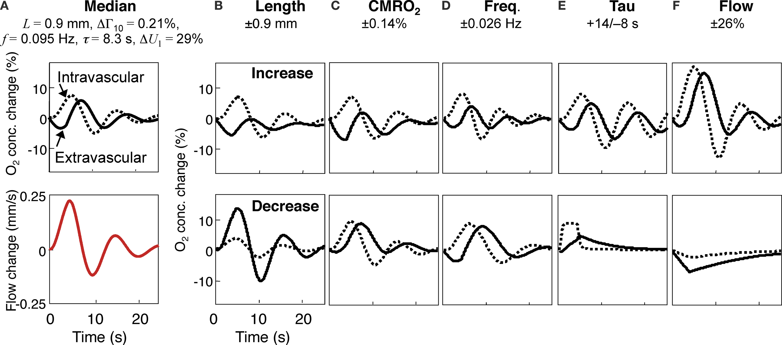
The model produced plausible results for the extravascular oxygen concentration corresponding to the two perturbations (Figure
3
, solid lines). The temporal responses for the extravascular oxygen concentration perturbation are shown in Figure
3
A for the median parameter set corresponding to the experimental fits to the entire dataset of 21 cells described below (
L = 0.9 mm, Γ
10/Γ
0 = 0.21%,
U10/
U0 = 29%,
f = 0.095 Hz, and τ = 8.3 s). The fits show an initial oxygen decrease caused by the 4-s-long pulse of CMRO
2 increase, followed by a positive phase of oxygen increase produced by the flow response together with subsequent under-damped oscillations. The intravascular flow response, shown in red, is fairly prompt, corresponding to the damped sinusoidal impulse response convolved with the 4-s-duration rect-function stimulus duration. We also illustrate the corresponding intravascular oxygen concentration changes (Figure
3
, dashed lines). The oxygen concentration results are distinctly different in the intravascular compartment, in that the deoxygenation phase is smaller or absent.
Figure 3. Effects of the five parameters on the model oxygen response. (A) top panel shows median response for both extravascular (solid line) and intravascular compartments (dashed line), bottom panel shows median flow response; (B) model results for both compartments corresponding to a one-standard deviation increase (top panels) and decrease (bottom panels) in the length parameter; (C) similar results for the CMRO2 perturbation parameter; (D) similar results for the flow-frequency parameter; (E) for the flow-damping parameter; (F) for the flow-magnitude parameter.
We investigated the effects of the five parameters by plotting the model output as each parameter was increased and decreased from its median value by its standard deviation across the experimental data (Figures
3
B–F). The length parameter (
L, Figure
3
B) has a global impact, with greater lengths increasing the effects of the extravascular CMRO
2 perturbation as well increasing transit-delay and smoothing. The magnitude of the CMRO
2 perturbation (Γ
1, Figure
3
C) has a much more temporally specific effect, directly modulating the magnitude of the early deoxygenation portion of the response. Note how the deoxygenation effects oppose the flow effects, so that an increased CMRO
2 perturbation decreases the magnitude of the initial flow-generated hyperoxic peak and vice-versa. The long delays to the hyperoxic peak are also a consequence of this competition. The flow frequency parameter (
f, Figure
3
D) modulates the frequency of the underdamped ringing, but also affects the width of the initial oxygen overshoot. The flow damping parameter (τ, Figure
3
E) directly affects the amount of ringing evident in the oxygen response; most measurements showed substantial ringing. The flow perturbation magnitude parameter (
U10, Figure
3
F) globally modulates the flow effects over the whole of the time course. Note that only when the flow is very small (Figure
3
F, lower panel) does the intravascular oxygen concentration drop below the equilibrium concentration. Generally, our model does not predict an “initial dip” in the intravascular compartment.
Fits to Experimental Data
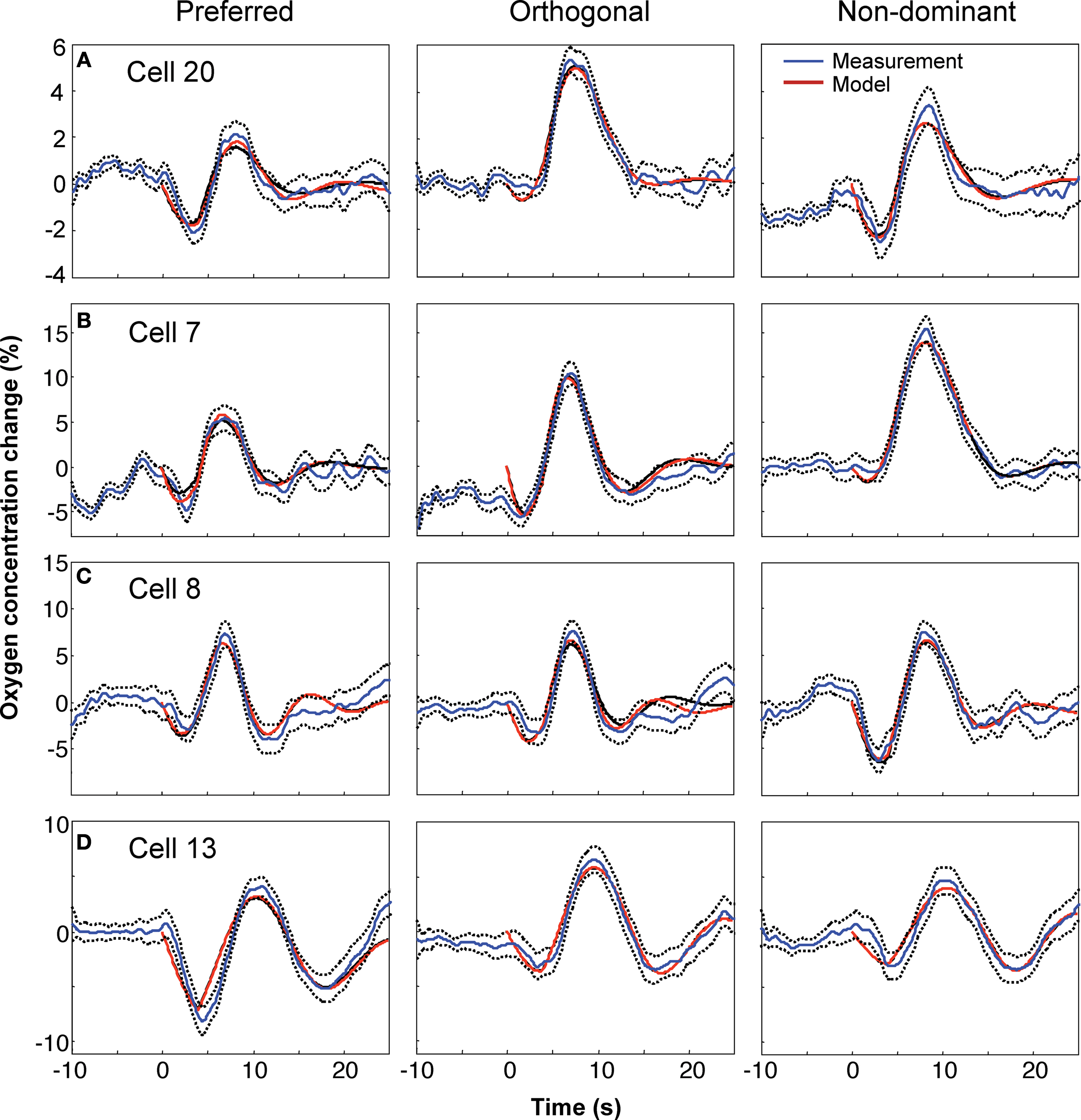
The model was capable of fitting the diverse dynamics of the experimentally observed tissue oxygen variations, as illustrated by examples from four different cell recordings (Figure
4
). Each row corresponds to a different cell. The leftmost column is the measurement and fit corresponding to the grating orientation that evoked the maximal neuronal response (“preferred” stimulus), the center column for the orthogonally oriented grating, and right column for the preferred-orientation stimulus presented to the non-dominant eye.
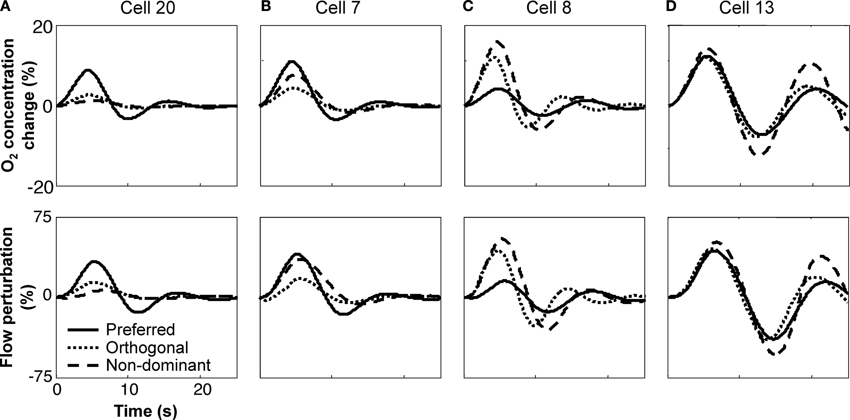
Figure 4. Model fits and experimental data for four cells and three stimulus configurations: (A) cell 20; (B) cell 7; (C) cell 8; (D) cell 13. For each cell, the left panel corresponds to the “preferred” orientation that evoked maximum firing, the middle panel to the orientation orthogonal to the preferred, and the right panel to the preferred orientation presented to the non-dominant eye. Mean experimental measurement is shown by the thin blue line, with standard error indicated by the surrounding dotted lines. Fits are shown by the thick lines, maximum-likelihood in red, least-squares in black; note that the fits are often so similar that they cannot be distinguished in the plots.
Fits to the measurements highlighted in
Thompson et al. (2003)
are shown in Figure
4
A, and corresponding intravascular flow and oxygen perturbations are shown in Figure
5
A. During the stimulus period, the CMRO
2 increases promptly, competing with the comparatively sluggish inflow of oxygenated blood. Consequently, there is an initial decrease in extravascular oxygen concentration that is subsequently overwhelmed by inflow to produce an increase in oxygen concentration. Later, there is an undershoot caused directly by “ringing” in the flow perturbation: blood flow periodically decreases below baseline levels, and these changes cause similar decreases in oxygen concentration. As the flow perturbation damps out, the oxygen concentration returns to baseline.
Figure 5. Intravascular model predictions for the same four cells. (A) cell 20;
(B) cell 7;
(C) cell 8;
(D) cell 13. The upper panels correspond to model predictions for the intravascular oxygen concentration, while the lower panels shown predicted flow variations, both in percent relative the steady-state values. Each graph shows the variations for same three stimulus configurations presented in Figure
4
: preferred, orthogonal, and non-dominant.
Measurements in the vicinity of three other cells are also shown. Most exhibited stronger perturbation responses than those from Cell 20. While a few other cells also showed relatively strongly damped behavior (Figures
4
B and
5
B), strong “ringing” was often evident (Figures
4
C,D). The accurate fits to this behavior are a direct consequence of the FEW flow model, which allows underdamped flow perturbations (Figures
5
C,D).
The corresponding fit parameters for these four cells are shown in Table
1
. The parameters illustrate the diversity of the behavior and the fits. CMRO
2 perturbations vary from 0.07 to 0.80%; length parameter vary from 0.1 to 3.5 mm, damping times from 4.3 to 50 s, and flow perturbations from 5.1 to 60.1%. The frequency is comparatively stable, varying from 0.063 to 0.106. Despite the substantial variability of the fit parameters, most of the fit parameters show significant correlations with neuronal activity (see below).

Our model successfully fit ∼93% (156 out of 166) of the experimental measurements using the maximum-likelihood metric, and 92% (154/166) using the least-squares metric. Consideration of the fits to the entire dataset (Figures 1–21 in Supplementary Material), show an interesting variety of dynamics in the time courses. For example, fits to the oxygen measurements near Cell 3 (Figure 3 in Supplementary Material) exhibited the combination of relatively modest ringing and long length so that the deoxygenation phase decayed slowly and dominated the dynamics when the neuronal activity was strong. For this same cell, when the stimulus was switched to the non-dominant eye, the ringing became much more pronounced, suggesting that a different microvascular “circuit” had been engaged. Cell 10 (Figure 10 in Supplementary Material) exhibits a faster response (modeled as a shorter length), and a weak flow response. The ability of the model to fit such a variety of response waveforms gave us additional confidence in its utility. This simple model, a combination of early oxygen diffusion in competition with underdamped flow oscillation, offers a quantitative mechanistic description for over a hundred detailed oxygen time series.
In fact, even the unsuccessful fits were still fairly good, with errors never exceeding the success threshold by more than 39%. Measurements near Cell 14 (Figure 14 in Supplementary Material) were least well fit by the model, with five out of the eight stimuli successfully fit by the stricter (least-squared-error) metric. This cell exhibited a different dynamic: several early deoxygenation periods with the largest occurring later in time after the visual stimulus had ceased. It is notable that this cell also exhibited a high baseline-firing rate (5–7 spikes/s) compared to most other cells. Most of the other measurements that were not fit satisfactorily did not return to zero toward the end of the measurement period; these measurements were also relatively noisy.
The parameter values of the successful fits varied substantially across the many measurements of the full dataset. The variations were substantial both cell-to-cell and within stimulus type. We examined the cell-to-cell variations by forming a “cocktail mean” for each cell, that is, the mean value of each parameter across all stimulus orientations, and then calculated the standard deviation of these cocktail means across the 21 cells. The standard deviations were: length, 45%; O2 rate, 42%; flow frequency, 19%; damping time, 77%; flow magnitude, 61%. Within-cell variations across stimuli were obtained by normalizing each cell’s set of parameter values by its cocktail mean, and calculating the standard deviation; we then calculated the mean within-cell standard deviation across the ensemble of cells. The values were as follows: length, 56%; O2 rate, 33%; flow frequency, 15%; damping time, 51%; flow magnitude, 58%. With the exception of the length parameter, cell-to-cell variations were somewhat larger than within-cell (stimulus-to-stimulus) variations.
We also examined the effects of varying four other parameters: volume ratio (α), equilibrium flow velocity (U0), oxygen-extraction fraction (E), and equilibrium extravascular oxygen concentration (Qe00). In all cases, the results were similar for the quality of the fits to the extravascular oxygen measurements. However, adjusting these parameters had substantial effects on some of the five “free” model parameters. Because of the uncertainty in the sampling volume for oxygen probe, we refit the entire data set for α = 0.1 and 0.3, holding CBV constant at 0.06. Increasing the volume ratio decreases the “loading” of the extravascular volume on the diffusive losses from the intravascular volume. Consequently, the fits exhibit much greater length parameters (L) in order to match the temporal dynamics. Increasing α also causes a less pronounced decrease in the fitted flow perturbation magnitude (U10). Decreasing α has the reverse effect on both parameters. Each of the other three parameters was varied both above and below its nominal value by ∼15%, and the fitting procedure repeated. The main effect of changing Qe00 was to scale the magnitude of the perturbations in flow (U10) and CMRO2 (Γ10) required by the fits. Increasing Qe00 increases the equilibrium extravascular oxygen concentration near the end of the model cylinder. Consequently, the model fits require larger perturbations to fit the measurements. Decreasing E has much the same effect as increasing Qe00, but also reduces the longitudinal oxygen-concentration gradient. This, in turn, reduces the effect of convection relative to diffusion, changing the scaling between the two perturbations required to fit the measurements. Increasing U0 also increases the effect of convection relative to diffusion, and modifies the scaling between the two perturbations. All of these changes slightly modify the length parameter (L), but do not much affect the flow frequency or damping parameters. Thus, although these parameters had little effect on the quality of the fits to the extravascular oxygen measurements, they can substantially affect the intravascular dynamics.
Correlations with Neuronal Activity
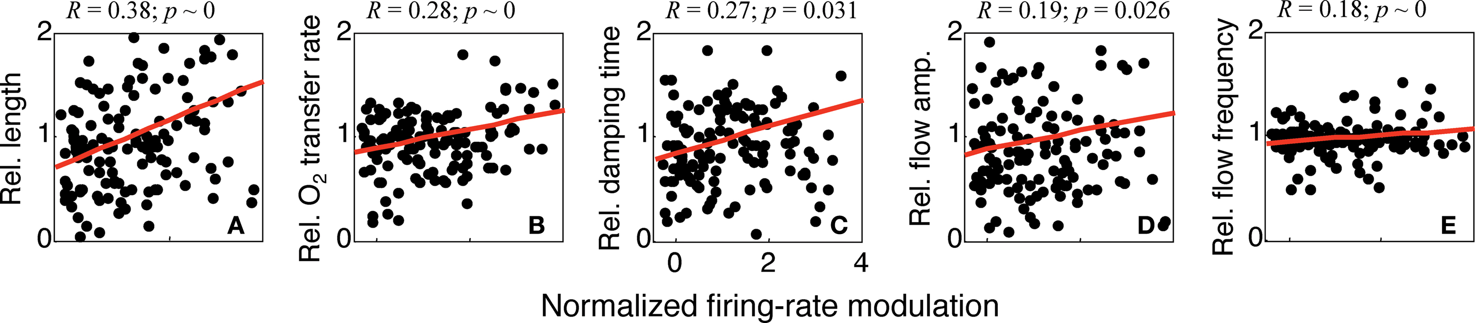
We examined the correlation of the parameters for successful fits with neuronal activity in the following fashion. Spike-rate modulations were calculated as the difference between the mean baseline firing rate and the mean firing rate during the stimulus presentation period. We divided each cell’s collection of spike-rate modulations and corresponding parameter values by their cocktail mean to compensate for cell-to-cell variations. We then plotted each normalized parameter value against the corresponding normalized spike-rate modulation (Figure
6
). All of the five parameters showed significant correlations with neuronal activity. The length parameter,
L, had the strongest correlation (
R = 0.38, infinitesimal
p). indicating that stronger firing is associated with slower oxygen dynamics. The oxygen-transfer rate, Γ
10, showed a weaker but still significant correlation (
R = 0.28, infinitesimal
p), consistent with the correlations reported by
Thompson et al. (2003)
. A positive correlation (
R = 0.27,
p = 0.031) with neuronal firing was also evident for the decay time constant, τ, indicating that the “ringing” increases with firing-rate modulation. A weak correlation (
R = 0.19,
p = 0.026) was also observed for the normalized flow magnitude,
U10, suggesting that neuronal activity also drives the flow perturbation. Finally, the flow frequency shows a positive correlation (
R = 0.18, infinitesimal
p), indicating that the ringing frequency increases with neuronal activity. However, the slope of this correlation is very small, so this is a weak effect.
Figure 6. Variations in parameter values with firing-rate modulation for all successfully fit measurements. (A) oxygen-transfer rate; (B) damping time; (C) length; (D) flow frequency; (E) flow magnitude. Parameter values and firing-rate modulation have all been normalized by their cocktail mean for each cell.
Our model for transient tissue oxygen delivery in cerebral cortex successfully fits a large dataset of extravascular oxygen measurements corresponding to brief visual stimulations. The model offers several useful features. First, it provides a very concise description of oxygen transport as a competition between prompt local oxygen diffusion and a spatially distributed underdamped flow response. Although elements of this model are similar to some previous models, the incorporation of the FEW flow model tremendously improves its explanatory power. Because the model offers accurate fits in a concise, five-parameter framework, certain aspects of the hemodynamic response can be understood by examining variations of the model parameters with neuronal firing-rate. Second, the model offers a mechanism that unifies the hemodynamic response with some components of the frequently observed phenomena of “spontaneous fluctuations” or “vasomotion.” This FEW flow model naturally incorporates underdamped flow perturbations, providing a simple mechanism for the observed late-time oscillations at ∼0.1 Hz that have not been well understood and modeled previously. Finally, the model also provides a description of the intravascular oxygen response that could yield some new insights into the hemodynamic response measured by BOLD functional magnetic resonance imaging (fMRI).
Our model provides mechanisms for the four temporal phases of the hemodyamic response: (1) The initial period of latency or dip observed in oxygen-sensitive hemodynamic measurements. The model gives a quantitative mechanism for this period as a competition between inflowing oxygenated blood, driven by the flow transient and delayed by propagation, and oxygen uptake. (2) The hyperoxic peak, also driven by the flow transient, which competes with and eventually overwhelms the oxygen consumption. (3) The undershoot, which is explained here as a brief flow decrease caused by the “ringing” dynamics of the FEW. (4) Subsequent oscillatory phenomena, which is explained as continued ringing in the flow model.
Valabregue et al. (2003)
suggested a model with similar geometry and oxygen-transport dynamics. Their model included the non-linear relationship between oxygen and oxyhemoglobin concentration in the intravascular compartment, as compared to the linear assumption of our own model. However, they did not include a flow model corresponding to a brief neural stimulation, nor did they attempt to fit experimental measurements of the transient hemodynamic oxygen response. To our knowledge, we offer the first attempt to fit such a model to the slow, event-related measurements of the sort obtained by
Thompson et al. (2003)
.
A model combining convection-diffusion oxygen transport with windkessel flow was fit to experimental optical imaging data by
Huppert et al. (2007)
with excellent results. However, there were some notable differences between that effort and our own. First, they used a delayed-compliance windkessel model rather than the FEW. Second, they used a more complex model that involved many parameters, so a much more intricate fitting procedure was required. Third, and most important, they applied their model to data from a fast event-related stimulus design and only fit the first 7 s of the experimental response. This approach has the effect of filtering out low-frequency variations that were so prevalent in the experimental results of
Thompson et al. (2003)
. It is therefore difficult to compare the efficacy of these two models across such disparate experimental data sets.
Our model does not utilize a non-linear flow-volume scaling relationship, such as Grubb’s power-law relationship (
Grubb et al., 1974
), used in many other models (
Buxton and Frank, 1997
;
Buxton et al., 1998
,
2004
;
Hyder et al., 1998
;
Zheng et al., 2002
,
2005
). Such scaling relations were obtained during experiments that took place on much slower time scales than the present experimental dataset. We suggest that the hemodynamics modeled here are distinct from cerebral auto-regulation, with the former mediated by microvascular control mechanisms on a relatively fast time scale (s), while the latter is mediated by smooth-muscle fibers that surround larger arteries on a slower time scale (tens of seconds). If so, it is likely that the mechanisms work in parallel, and both must be considered during experiments that manipulate the hemodynamic response.
The mean parameter values for our model present an interesting picture of microvascular hemodynamics. The median length parameter is 0.9 mm, which is consistent with oxygen transport from arterioles as well as capillaries, as has been previously suggested (
Sharan et al., 1989
;
Vovenko, 1999
;
Zheng et al., 2005
), with upstream control points located along the arteriolar tree. This result is also consistent with tissue oxygen measurements from the lateral geniculate nucleus suggest that the point spread function of the flow response has a width of approximately 1.4 mm (
Thompson et al., 2005
). However, our length parameters are only rough estimates, because the simple geometry of our model does not take into account the variations in diameter and flow velocity that occur within the vascular tree. The median frequency parameter in the flow model, 0.10 Hz, was quite stable, suggesting that the pial vascular network behaves as a second-degree, roughly linear filter that is mechanically tuned to a particular frequency. Moreover, the median damping time of ∼8 s suggests that this network has an underdamped, bandpass character, with several cycles of “ringing” a normal aspect of the hemodynamic response.
The variation of our model parameters with firing-rate modulation provides some insight into the character of the hemodynamic response to brief neural stimulation. Our model indicates significant correlations between both oxygen demand and the flow perturbation with local neuronal firing (Figures
6
A,D). Both correlations are consistent with the usual notions of neurovascular coupling. The correlation of our length parameter
L on firing-rate modulation (Figure
6
A) enriches this picture. The tendency toward larger length parameters with increasing firing-rate modulation suggests that stronger neuronal activity tends to attract blood flow from a broader region of vascular control. Finally, the significant correlation of damping time with spike rate modulation (Figure
6
B) suggests that the observed underdamped ringing effects are an integral part of the hemodynamic response. Strong spike-rate modulation appears to drive strong ringing.
Our flow model suggests an alternative explanation for some of the low-frequency oscillations or “vasomotion” observed with various techniques, e.g. (
Katura et al., 2006
;
Kleinfeld et al., 1998
;
Koepchen, 1984
;
Mayhew et al., 1996
;
Spitzer et al., 2001
), including the present tissue oxygen measurements (
Thompson et al., 2003
). Generally, these slow hemodynamic fluctuations have been attributed to other mechanisms such as blood pressure feedback from baroreceptors or neurogenic mechanisms. These fluctuations, sometimes called Mayer waves, are observed in three frequency bands. The so-called “low-frequency” (LF) band of such fluctuations occurs at ∼0.1 Hz, making it particularly relevant to the measurements and model presented here. The FEW has a bandpass response to transient changes in cerebrovascular control. Thus, unstimulated or spontaneous neural activity would be filtered by the hemodynamic network to appear as low-frequency oscillations in flow, oxygen transport, and other aspects of the hemodynamics. This hypothesis is consistent with the use of low-frequency fluctuations as a “resting-state” measurement of neural activity using fMRI (
Biswal et al., 1997
;
Fransson, 2005
;
Peltier and Noll, 2002
). The purpose of these oscillations is not yet understood. It has been suggested that low-frequency oscillations could increase oxygen transport efficacy (
Goldman and Popel, 2001
;
Kislukhin, 2004
). Alternatively, the advantage of underdamping may simply be that of speed. Given our simple second-degree flow model, an underdamped flow response provides more immediate and copious delivery of oxygenated blood than a critically damped response.
It could also be that several mechanisms are responsible for these fluctuations, with the FEW responsible only for fluctuations in hemodynamics associated with transient neural activation, while the usual neural feedback mechanisms are responsible for oxygen auto-regulatory functions. It is also possible that the two mechanisms are related, with the tuned bandpass character of the cerebral vasculature actually a consequence of the putative neurogenic feedback mechanisms. Although in global scope, the mechanism of the LF fluctuations may be complex and non-linear (
Seydnejad and Kitney, 2001
), at the level of the present cerebrovascular oxygen measurements they may be satisfactorily described by the FEW linear model. In this view, the dynamics of the FEW are an abstract model of more complex feedback mechanisms rather than a literal model of simple mechanical processes. Further experiments will be necessary to elucidate the relationship between the FEW and LF fluctuations.
The CMRO
2 changes predicted by the model are much smaller than measured values [e.g., ∼10% observed using PET (
Ito et al., 2005
)]. This underestimate could reflect the model’s assumption that oxygen demand increases uniformly along the entire length of the model. In reality the demand could increase in a more localized fashion corresponding only to the active portions of the parenchyma. Moreover, this simple model represents the dynamics of the entire arteriolar tree with a single flow velocity, so it may not be possible to consistently match predictions for both velocity and CMRO
2 perturbations to measurements. Finally, this distortion could also be caused by our assumption of linear hemoglobin oxygen dissociation.
Our model also makes interesting but tentative predictions about the character of the intravascular flow and oxygen responses to brief neural stimulation. With the baseline set of fixed parameters (α,
Qe00,
E, and
U0), the predicted flow changes have a mean value of 26%, which is similar to measurements, e.g., the ∼30% flow changes obtained by positron emission tomography and MRI (
Feng et al., 2004
;
Fox and Raichle, 1984
). However, neglecting the non-linearity in oxygen dissociation could significantly distort the model’s detailed predictions of the intravascular dynamics. This could bear on the model’s prediction of little or no “initial dip” in the intravascular oxygen concentration. Because the non-linearity “stiffens” the oxygen transfer from the erythrocytes to the vessel wall, the response to the initial period of oxygen demand may be larger than predicted.
The intravascular aspects of our model will form the basis for a model of the BOLD fMRI hemodynamic impulse response. To do so, the current model’s predictions of oxygen concentration would be coupled to the additional dynamics of intravascular oxygen dissociation to obtain estimates of oxygenated and deoxygenated hemoglobin concentrations. These estimates, in turn, would be linked to a model of MR sampling to quantify the intravascular and extravascular components of the BOLD response. Finally, the current model’s linear flow response system would form the basis for an estimate of the fMRI volume response component.
D. Ress conceived this model, performed the mathematical analysis, wrote the initial numerical solution and fitting procedures, and performed the fits to the experimental data. J. Thompson collected the experimental data, organized it into a convenient form, and provided critical assistance on its use and interpretation. B. Rokers converted the initial Matlab code into C, tremendously increasing the speed of the fitting process. R. Khan performed an extensive investigation of the effects of the volume-ratio parameter (α) on the fits. A. Huk provided the maximum-likelihood fitting procedure. All authors assisted in writing this manuscript. There was no “senior” author.
Appendix: Derivation of the Oxygen-Transport Equations
Consider a three-compartment cylindrical system representing the intravascular, extravascular, and intracellular spaces, with radii r1, r2, and r3, respectively. If we allow variation only along the z-axis, we can treat oxygen transport from disc- or annulus-shaped regions of differential thickness Δz. In the intravascular compartment, the loss of oxygen molecules, Mi, is the sum of oxygen removed by flow plus the losses caused by diffusion into the extravascular compartment:
where
P and Δ
w are the permeability and thickness of the vascular wall, respectively, and the oxygen concentrations,


In the extravascular compartment, the oxygen gain is driven by diffusion into the compartment minus losses into the intracellular compartment:
where Γ represents CMRO2 in molecules per unit-time per volume. Dividing out the volumes, taking limits, and rearranging gives:
This is the same as Eq. 1 with explicit definitions of the constants,
A = 2
P/r
1Δ
w,
and

Note that we can rewrite

where CBV is the cerebral blood volume fraction.
Conflict of Interest Statement
The authors declare that the research was conducted in the absence of any commercial or financial relationships that could be construed as a potential conflict of interest.
The authors thank Ralph Freeman for providing the experimental data used in this work.
The Supplementary Material for this article can be found online at
http://webspace.utexas.edu/dr9774/O2transportData.pdf
.
Biswal, B. B., Van Kylen, J., and Hyde, J. S. (1997). Simultaneous assessment of flow and BOLD signals in resting-state functional connectivity maps.
NMR Biomed. 10, 165–170.
Burattini, R., and Di Salvia, P. O. (2007). Development of systemic arterial mechanical properties from infancy to adulthood interpreted by four-element windkessel models.
J. Appl. Physiol. 103, 66–79.
Buxton, R. B., and Frank, L. R. (1997). A model for the coupling between cerebral blood flow and oxygen metabolism during neural stimulation.
J. Cereb. Blood Flow Metab. 17, 64–72.
Buxton, R. B., Uludag, K., Dubowitz, D. J., and Liu, T. T. (2004). Modeling the hemodynamic response to brain activation.
Neuroimage 23(Suppl. 1), S220–233.
Buxton, R. B., Wong, E. C., and Frank, L. R. (1998). Dynamics of blood flow and oxygenation changes during brain activation: the balloon model.
Magn. Reson. Med. 39, 855–864.
Cassot, F., Lauwers, F., Fouard, C., Prohaska, S., and Lauwers-Cances, V. (2006). A novel three-dimensional computer-assisted method for a quantitative study of microvascular networks of the human cerebral cortex.
Microcirculation 13, 1–18.
Feng, C. M., Narayana, S., Lancaster, J. L., Jerabek, P. A., Arnow, T. L., Zhu, F., Tan, L. H., Fox, P. T., and Gao, J. H. (2004). CBF changes during brain activation: fMRI vs. PET.
Neuroimage 22, 443–446.
Fox, P. T., and Raichle, M. E. (1984). Stimulus rate dependence of regional cerebral blood flow in human striate cortex, demonstrated by positron emission tomography.
J. Neurophysiol. 51, 1109–1120.
Fransson, P. (2005). Spontaneous low-frequency BOLD signal fluctuations: an fMRI investigation of the resting-state default mode of brain function hypothesis.
Hum. Brain Mapp. 26, 15–29.
Goldman, D., and Popel, A. S. (2001). A computational study of the effect of vasomotion on oxygen transport from capillary networks.
J. Theor. Biol. 209, 189–199.
Grubb, R. L. Jr, Raichle, M. E., Eichling, J. O., and Ter-Pogossian, M. M. (1974). The effects of changes in PaCO2 on cerebral blood volume, blood flow, and vascular mean transit time.
Stroke 5, 630–639.
Harrison, R. V., Harel, N., Panesar, J., and Mount, R. J. (2002). Blood capillary distribution correlates with hemodynamic-based functional imaging in cerebral cortex.
Cereb. Cortex 12, 225–233.
Hayashi, T., Watabe, H., Kudomi, N., Kim, K. M., Enmi, J., Hayashida, K., and Iida, H. (2003). A theoretical model of oxygen delivery and metabolism for physiologic interpretation of quantitative cerebral blood flow and metabolic rate of oxygen.
J. Cereb. Blood Flow Metab. 23, 1314–1323.
Herman, P., Trubel, H. K., and Hyder, F. (2006). A multiparametric assessment of oxygen efflux from the brain.
J. Cereb. Blood Flow Metab. 26, 79–91.
Hudetz, A. G. (1999). Mathematical model of oxygen transport in the cerebral cortex.
Brain Res. 817, 75–83.
Huppert, T. J., Allen, M. S., Benav, H., Jones, P. B., and Boas, D. A. (2007). A multicompartment vascular model for inferring baseline and functional changes in cerebral oxygen metabolism and arterial dilation.
J. Cereb. Blood Flow Metab. 27, 1262–1279.
Hyder, F., Shulman, R. G., and Rothman, D. L. (1998). A model for the regulation of cerebral oxygen delivery.
J. Appl. Physiol. 85, 554–564.
Ito, H., Ibaraki, M., Kanno, I., Fukuda, H., and Miura, S. (2005). Changes in cerebral blood flow and cerebral oxygen metabolism during neural activation measured by positron emission tomography: comparison with blood oxygenation level-dependent contrast measured by functional magnetic resonance imaging.
J. Cereb. Blood Flow Metab. 25, 371–377.
Ito, H., Kanno, I., Kato, C., Sasaki, T., Ishii, K., Ouchi, Y., Iida, A., Okazawa, H., Hayashida, K., Tsuyuguchi, N., Ishii, K., Kuwabara, Y., and Senda, M. (2004). Database of normal human cerebral blood flow, cerebral blood volume, cerebral oxygen extraction fraction and cerebral metabolic rate of oxygen measured by positron emission tomography with 15O-labelled carbon dioxide or water, carbon monoxide and oxygen: a multicentre study in Japan.
Eur. J. Nucl. Med. Mol. Imaging 31, 635–643.
Katura, T., Tanaka, N., Obata, A., Sato, H., and Maki, A. (2006). Quantitative evaluation of interrelations between spontaneous low-frequency oscillations in cerebral hemodynamics and systemic cardiovascular dynamics.
Neuroimage 31, 1592–1600.
Kislukhin, V. V. (2004). Regulation of oxygen consumption by vasomotion.
Math. Biosci. 191, 101–108.
Kleinfeld, D., Mitra, P. P., Helmchen, F., and Denk, W. (1998). Fluctuations and stimulus-induced changes in blood flow observed in individual capillaries in layers 2 through 4 of rat neocortex.
Proc. Natl. Acad. Sci. U.S.A. 95, 15741–15746.
Kobari, M., Gotoh, F., Fukuuchi, Y., Tanaka, K., Suzuki, N., and Uematsu, D. (1987). Quantitative measurement of blood flow velocity in feline pial arteries during hemorrhagic hypotension and hypercapnia.
Stroke 18, 457–463.
Koepchen, H. P. (1984). History of studies and concepts of blood pressure waves. In Mechanisms of Blood Pressure Waves, K. Miyakawa, H. P. Koepchen and C. Polosa, eds (New York, Springer-Verlag), pp. 3–27.
Ladurner, G., Zilkha, E., Iliff, D., du Boulay, G. H., and Marshall, J. (1976). Measurement of regional cerebral blood volume by computerized axial tomography.
J. Neurol. Neurosurg. Psychiatr. 39, 152–158.
Lagarias, J. C., Reeds, J. A., Wright, M. H., and Wright, P. E. (1998). Convergence properties of the Nelder-Mead simplex method in low dimensions.
SIAM J. Optim. 9, 112–147.
Malonek, D., Dirnagl, U., Lindauer, U., Yamada, K., Kanno, I., and Grinvald, A. (1997). Vascular imprints of neuronal activity: relationships between the dynamics of cortical blood flow, oxygenation, and volume changes following sensory stimulation.
Proc. Natl. Acad. Sci. U.S.A. 94, 14826–14831.
Mandeville, J. B., Marota, J. J., Ayata, C., Zaharchuk, G., Moskowitz, M. A., Rosen, B. R., and Weisskoff, R. M. (1999). Evidence of a cerebrovascular postarteriole windkessel with delayed compliance.
J. Cereb. Blood Flow Metab. 19, 679–689.
Mayhew, J. E., Askew, S., Zheng, Y., Porrill, J., Westby, G. W., Redgrave, P., Rector, D. M., and Harper, R. M. (1996). Cerebral vasomotion: a 0.1-Hz oscillation in reflected light imaging of neural activity.
Neuroimage 4, 183–193.
Mintun, M. A., Lundstrom, B. N., Snyder, A. Z., Vlassenko, A. G., Shulman, G. L., and Raichle, M. E. (2001). Blood flow and oxygen delivery to human brain during functional activity: theoretical modeling and experimental data.
Proc. Natl. Acad. Sci. U.S.A. 98, 6859–6864.
Nicholson, C., and Sykova, E. (1998). Extracellular space structure revealed by diffusion analysis.
Trends Neurosci. 21, 207–215.
Olson, H. F. (1943). Dynamical Analogies. New York, D. Van Nostrand Company, Inc.
Peltier, S. J., and Noll, D. C. (2002). T(2)(*) dependence of low frequency functional connectivity.
Neuroimage 16, 985–992.
Phelps, M. E., Huang, S. C., Hoffman, E. J., and Kuhl, D. E. (1979). Validation of tomographic measurement of cerebral blood volume with C-11-labeled carboxyhemoglobin.
J. Nucl. Med. 20, 328–334.
Rodriguez-Baeza, A., Reina-De La Torre, F., Ortega-Sanchez, M., and Sahuquillo-Barris, J. (1998). Perivascular structures in corrosion casts of the human central nervous system: a confocal laser and scanning electron microscope study.
Anat. Rec. 252, 176–184.
Rusakov, D. A., and Kullmann, D. M. (1998). Geometric and viscous components of the tortuosity of the extracellular space in the brain.
Proc. Natl. Acad. Sci. U.S.A. 95, 8975–8980.
Seydnejad, S. R., and Kitney, R. I. (2001). Modeling of Mayer waves generation mechanisms.
IEEE Eng. Med. Biol. Mag. 20, 92–100.
Sharan, M., Jones, M. D. Jr, Koehler, R. C., Traystman, R. J., and Popel, A. S. (1989). A compartmental model for oxygen transport in brain microcirculation.
Ann. Biomed. Eng. 17, 13–38.
Spitzer, M. W., Calford, M. B., Clarey, J. C., Pettigrew, J. D., and Roe, A. W. (2001). Spontaneous and stimulus-evoked intrinsic optical signals in primary auditory cortex of the cat.
J. Neurophysiol. 85, 1283–1298.
Stergiopulos, N., Westerhof, B. E., and Westerhof, N. (1999). Total arterial inertance as the fourth element of the windkessel model.
Am. J. Physiol. 276, H81–H88.
Thiry, P. S., and Roberge, F. A. (1976). Analogs and models of systemic arterial circulation.
Rev. Can. Biol. 35, 217–238.
Thompson, J. K., Peterson, M. R., and Freeman, R. D. (2003). Single-neuron activity and tissue oxygenation in the cerebral cortex.
Science 299, 1070–1072.
Thompson, J. K., Peterson, M. R., and Freeman, R. D. (2005). Separate spatial scales determine neural activity-dependent changes in tissue oxygen within central visual pathways.
J. Neurosci. 25, 9046–9058.
Tsai, A. G., Friesenecker, B., Mazzoni, M. C., Kerger, H., Buerk, D. G., Johnson, P. C., and Intaglietta, M. (1998). Microvascular and tissue oxygen gradients in the rat mesentery.
Proc. Natl. Acad. Sci. U.S.A. 95, 6590–6595.
Tsai, A. G., Johnson, P. C., and Intaglietta, M. (2003). Oxygen gradients in the microcirculation.
Physiol. Rev. 83, 933–963.
Valabregue, R., Aubert, A., Burger, J., Bittoun, J., and Costalat, R. (2003). Relation between cerebral blood flow and metabolism explained by a model of oxygen exchange.
J. Cereb. Blood Flow Metab. 23, 536–545.
Vanzetta, I., and Grinvald, A. (1999). Increased cortical oxidative metabolism due to sensory stimulation: implications for functional brain imaging.
Science 286, 1555–1558.
Vovenko, E. (1999). Distribution of oxygen tension on the surface of arterioles, capillaries and venules of brain cortex and in tissue in normoxia: an experimental study on rats.
Pflugers Arch. 437, 617–623.
Zheng, Y., Johnston, D., Berwick, J., Chen, D., Billings, S., and Mayhew, J. (2005). A three-compartment model of the hemodynamic response and oxygen delivery to brain.
Neuroimage 28, 925–939.
Zheng, Y., Martindale, J., Johnston, D., Jones, M., Berwick, J., and Mayhew, J. (2002). A model of the hemodynamic response and oxygen delivery to brain.
Neuroimage 16, 617–637.