Massively parallel signal processing using the graphics processing unit for real-time brain–computer interface feature extraction
Department of Biomedical Engineering, University of Wisconsin-Madison, Madison, WI, USA
The clock speeds of modern computer processors have nearly plateaued in the past 5 years. Consequently, neural prosthetic systems that rely on processing large quantities of data in a short period of time face a bottleneck, in that it may not be possible to process all of the data recorded from an electrode array with high channel counts and bandwidth, such as electrocorticographic grids or other implantable systems. Therefore, in this study a method of using the processing capabilities of a graphics card [graphics processing unit (GPU)] was developed for real-time neural signal processing of a brain–computer interface (BCI). The NVIDIA CUDA system was used to offload processing to the GPU, which is capable of running many operations in parallel, potentially greatly increasing the speed of existing algorithms. The BCI system records many channels of data, which are processed and translated into a control signal, such as the movement of a computer cursor. This signal processing chain involves computing a matrix–matrix multiplication (i.e., a spatial filter), followed by calculating the power spectral density on every channel using an auto-regressive method, and finally classifying appropriate features for control. In this study, the first two computationally intensive steps were implemented on the GPU, and the speed was compared to both the current implementation and a central processing unit-based implementation that uses multi-threading. Significant performance gains were obtained with GPU processing: the current implementation processed 1000 channels of 250 ms in 933 ms, while the new GPU method took only 27 ms, an improvement of nearly 35 times.
The last 5 years has seen an increase in implantable electrode technology for brain–computer interfaces (BCIs) in humans (Felton et al., 2007
; Kim et al., 2008
; Leuthardt et al., 2004
; Schalk et al., 2008b
; Wilson et al., 2006
), in particular the use of electrocorticographic (ECoG) electrodes. From a signal processing and control standpoint, ECoG is a superior choice for BCIs compared to electroencephalogram (EEG), because the cortical signal sources are much closer to the electrodes. This results in (1) a signal of higher amplitude by several orders of magnitude, (2) increased spatial resolution due to decreased blurring from volume conduction through the tissue and bone surrounding the brain, and (3) a higher frequency content in the signal. Standard EEG has amplitudes of tens of μV, spatial resolution on the order of cm, and a frequency bandwidth of 0–40 Hz, while ECoG has amplitudes of hundreds of μV, a spatial resolution on the mm scale, and contains relevant physiological information >200 Hz (Crone et al., 2006
; Schalk et al., 2008b
; Wilson et al., 2006
). Additionally, ECoG implants typically contain 64 or more channels, increasing the potential amount of information beyond what is possible with EEG.
The drawback to all of this information is what to do with it, or more specifically how to do something with it. The higher bandwidth necessitates a higher sampling frequency, often above 1 kHz. ECoG-based BCIs use voluntary changes in the sensorimotor rhythms (mu, beta, gamma, and high-gamma) as the control signal, and the most common signal processing method is to calculate the power spectra on several channels in “real-time,” or approximately 20–30 times per second. After including the other processing and classification steps, such as spatial filtering, the central processing unit (CPU) in a computer may begin having trouble processing large numbers of high-bandwidth signals quickly enough to maintain real-time capability.
As processor clock speeds have plateaued recently due to issues with heat dissipation and the time required for transistors to accumulate and dissipate charge, the primary method of achieving increased performance has been found by adding cores to the processor in lieu of increasing the individual CPU speed itself (NVIDIA, 2008b
). Each core is capable of executing an independent thread of execution, allowing the operating system and individual programs to perform several tasks simultaneously on multiple “slower” cores, instead of running several tasks sequentially on a single fast core. Therefore, most commercially available processors currently include at least two cores, and some have up to eight (e.g., the Mac Pro with two quad-core CPUs). This emphasis on parallel processing lends itself well to signal processing in BCIs, which can operate on individual channels simultaneously to utilize multi-core technology. However, even in the best-case scenario in which all eight cores are available to the BCI program, if it is necessary to operate on 64+ channels, significant portions of the processing chain will be performed in series, not in parallel. As the channel count and sampling rates increase, and processing algorithms become more complex, even eight cores may not be able to keep up for a real-time system. In recent ECoG-based BCI studies, only a small subset of channels are utilized for control (Leuthardt et al., 2004
; Schalk et al., 2008b
; Wilson et al., 2006
) , or long update periods (100 ms or longer)are used to allow all data to be processed (Schalk et al., 2008a
). All of these examples would benefit directly from methods that increase the processing capabilities of the BCI system.
A few alternatives exist. The first is to move the BCI system to dedicated hardware that is capable of processing the data as needed. The drawback to this is that it is often much more difficult to develop and maintain a hardware-based solution, and it becomes much more difficult to collaborate and compare data if a consistent platform is unavailable. The alternative to hardware solutions is a generic software solution, such as BCI2000 (Schalk et al., 2004
), which coordinates data acquisition from an amplifier, signal processing, and application output, all of which are run on a standard PC. The disadvantage to using a PC for a high-speed BCI system is that the BCI must compete with the operating system (e.g., Windows XP or Vista) for system resources, and may be pre-empted by other programs and processes for CPU time. BCI2000 is already a multi-process system, in which all stages in the signal chain run simultaneously; however, it is limited by the number of cores available on the machine, typically between 1 and 8. Until the number of cheaply available cores increases beyond 8, or the CPU speeds increase, any current PC-based solution will be limited by the number of channels and the sampling rate that can effectively be processed.
This study introduces a parallel processing paradigm in which the real-time signal processing algorithms are off-loaded from the CPU to the graphics processing unit (GPU), typically on the video card. Recently, the GPU chip manufacturer NVIDIA (Santa Clara, CA, USA) introduced a software interface called CUDA (Compute Unified Device Architecture) that allows massively parallel algorithms to be run on the video card GPU, which can contain dozens to hundreds of cores. This API is written in the C programming language, greatly simplifying the process of migrating existing CPU-based code to run using CUDA. The goal of this study is to measure the performance gains for different numbers of channels and samples processed using the CUDA system. Two algorithms from BCI2000 were implemented using CUDA: the spatial filter which performs a matrix multiplication of the neural data in order to re-reference the incoming signals (e.g., a common-average or Laplacian reference), and the power spectral estimate for all channels, which is calculated using an auto-regressive (AR) model. These results are compared to the BCI2000 single-threaded algorithms, and CPU-based multi-threaded algorithms.
Computer
An 8-core Apple Mac Pro was used for all tests. This system contains dual Intel Xeon quad-core processors, each with a clock speed of 2.8 GHz; the system had 6 GB of RAM. CUDA is platform-independent, and runs on Windows, Macs, and Linux computers. Experimental data was collected on this computer while running Mac OS X 10.5.5, Windows XP SP3, and Linux Ubuntu 8.10, each booted natively (i.e., virtualization software was not used).
Video Card
An NVIDIA 8800 GT video card was installed in a PCIe card slot. This card contains 112 cores running at 900 MHz, has 512 MB RAM, and can transfer up to 57.6 GB/s (NVIDIA, 2009
). Version 2.1 of the CUDA software was used.
BCI Signal Processing
Any BCI system is comprised of several common elements, regardless of the specific implementation and application. Neural signals are acquired from an amplification and digitization system, processed in several stages to produce an appropriate control signal, which drives the output device. The signal processing stages will vary depending on the application, e.g., control of a virtual cursor or a spelling application. In this study, we addressed algorithms specific to virtual cursor control, which are generally the most computationally intensive, and include a spatial filter, power spectral estimation, the linear combination of selected signal features to create the control signal output, and normalization of the control signal to the desired output range (Figure 1
). Of these, the spatial filter and power estimation require the most computational resources, both in terms of memory and processing time. The final three steps typically only require a few operations, and would not benefit significantly from GPU-based parallelization. Therefore, the goal of this study was to increase the performance of the spatial filter and the power estimation algorithms by designing parallel implementations to run both on multi-core CPUs and on the graphics card via the CUDA interface.

Figure 1. The signal processing flow in any brain–computer interface. Data recorded from the brain is processed in two general steps, comprised of feature extraction, which converts relevant brain features into an appropriate task-specific representation (e.g., frequency domain or time-domain average), and translation, which converts the brain features into a control signal. This paper focuses on the feature extraction portion, which is the most computationally extensive.
The first signal processing step, the spatial filter, relies on matrix multiplication, which is often referred to as an “embarrassingly parallel” problem (Foster, 1995
). That is, any element of the output signal is independent of all other elements; thus, it is possible to calculate each element in any order with very little synchronization, which can slow processing.
The second processing step, which uses an AR algorithm to find model coefficients and subsequently the power spectral density, does not present an immediate parallel solution because the process contains several sequential steps which depend on previously obtained values, and thus requires several synchronization points. In BCI2000, the Burg AR method is used, because it always produces stable coefficients (Andersen, 1978
; Burg, 1975
; Jansen et al., 1981
; Makhoul, 1975
). Here, a recursive procedure is used in which the model coefficients are re-estimated at each step, and with each iteration, several inter-dependent values are calculated, a simple process for serial processing within a single thread, but greatly complicated with the introduction of many threads running at the same time.
The details for each algorithm implementation are provided below, after an overview of GPU processing implementation.
GPU Implementation Overview
The parallel implementations for the algorithms presented are dependent on the underlying hardware used for performing the spatial filter and power spectra operations. While the methods used for matrix multiplication and calculating the AR coefficients are well-established (Press et al., 1999
), it is not necessarily trivial to port existing code intended to run on a single processor to run in potentially thousands of threads simultaneously. Furthermore, the graphics card architecture has a very different execution and memory model than traditional CPU-based systems with which most programmers are acquainted. Therefore, this section provides a general overview of the GPU device architecture, addressing methods for optimizing threaded execution and memory access on the graphics card. Detailed information on programming with CUDA can be found in the NVIDIA CUDA Programming Guide (NVIDIA, 2008b
).
As a simple example, consider a parallel power estimation implementation in which a single thread does all of the calculations for an individual channel; that is, the existing version of the algorithm, designed to run on a single processor, is more or less copied to run on the GPU with no changes. In this scenario, if one channel is processed, then only one thread is used, if 10 channels are processed, then 10 threads are used, etc. While this reduces the complexity of the resulting implementation, it also greatly underutilizes the GPU, which excels at performing many small tasks simultaneously, rather than one large task sequentially. CUDA uses an execution architecture called single-instruction, multiple-thread in which 32 threads (termed a warp) execute the same instructions in parallel, until either a synchronization point is reached, or the code branches in a manner dependent on the particular thread executing the code. Therefore, full efficiency is achieved when 32 threads have the same execution path, implying that a multiple of 32 number of threads should be used for any operation, and that all threads should be working at any given point in the code with minimal branching.
Groups of threads are organized into multi-dimensional computational blocks, providing a way to arrange threads into larger computational elements (Figure 2
). For example, a single block might contain 128 threads (a multiple of 32), and each thread in the block would be responsible for operating on individual data points in the algorithm. Thus, each block might be responsible for performing an entire calculation on a data vector by utilizing 128 threads to perform the computation.
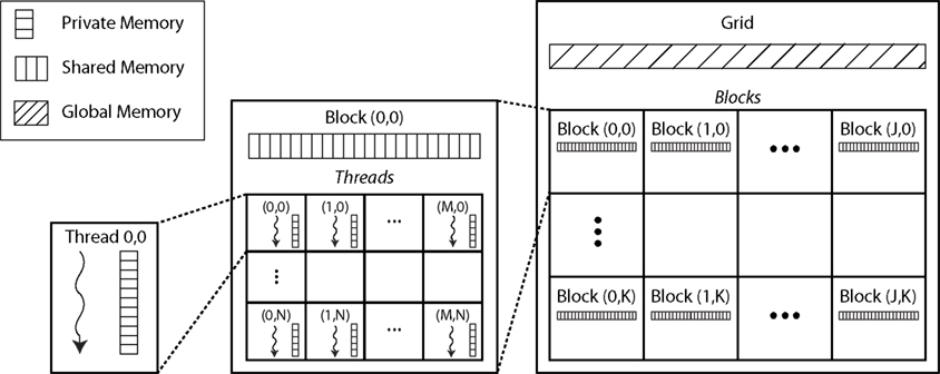
Figure 2. The organization of threads and memory hierarchy. Individual threads are organized into blocks, which are organized into a grid. Within a block, an individual thread has a unique three-component index which identifies its position in the block; similarly each block has a three-component index identifying its position in the grid. Each thread has a private local memory accessible only to that thread; every block has shared memory accessible to all threads in that block; and all threads can access global memory.
In addition to the threaded processing model, memory management plays a crucial role in computational efficiency. There are three levels of memory spaces available to threads. At the lowest level is the private local memory for each thread, in which temporary variables are created for use in an individual thread, and are not accessible outside of that thread. Next is the shared memory visible to all threads in a block, allowing many threads to work on the same memory simultaneously. At the highest level is the global, or device, memory, which is visible to all threads. It is most efficient to perform operations in shared memory, since it is located on the chip, and only requires 4 clock cycles to issue an instruction in shared memory; conversely, it can take between 400 and 600 clock cycles to access global memory, which can significantly slow down processing times. Therefore, it is generally necessary to copy the required segment of data from global memory to shared memory, perform the calculations and store the result in shared memory, and copy the result back to device memory at the end. The drawback to using shared memory is that there is limited amount available per block (up to 16384 bytes); therefore, operations on large data sets may require accessing and writing to global memory several times during execution, or operating primarily in global memory (Figure 2
).
It is clear that the computational methods developed for the single-thread model must be reconsidered to take advantage of the massively parallel GPU architecture. New data parallel primitives must be implemented and utilized in CUDA to efficiently replace serial algorithms. One such method is parallel reduction, which is used to iterate over a data series and produce a result. A simple problem that reduction can solve is the summation of many values in a vector:
While simple, this translates poorly to CUDA, because individual elements of the vector can only be accessed by a single thread at a time. Therefore, a better way to handle this problem is to use reduction, in which all threads are active at once, each adding up small pieces of the vector in shared memory. Using reduction it is possible to reduce the complexity of a problem from a O(N) operation to a O(log N) operation. Reduction is used in several instances in the algorithms presented in this study, and although a detailed discussion of reduction is beyond the scope of this paper, it is provided (with examples) in the CUDA software development kit (SDK) (NVIDIA, 2008b
).
This brief introduction to GPU programming concepts provides a basis for understanding the matrix multiplication and power spectral estimation algorithms developed. The implementation details for the spatial filter and power estimation follow, first for CPU-based multi-threaded systems, and then for the CUDA system.
Spatial Filter Overview
In order to fairly compare GPU-based matrix–matrix multiplication performance with a CPU-based implementation, a multi-threaded version of the spatial filter algorithm was developed to take advantage of modern multi-core processors.
Equation 1 shows the general equation for matrix–matrix multiplication:

where A is a Cin × S matrix, B is a Cout × Cin matrix, and C is a Cout × S matrix, where S is the number of samples, Cin is the number of input channels, and Cout is the number of resulting output channels. Then, element Cij of the output is:

If two matrices with dimensions of N × N are multiplied, then N3 operations are required to perform the multiplication. Therefore, small increases in the number of elements can result in increasingly large computation times. In BCI applications, the matrices are not usually square: the signal matrix has dimensions of Cin × S, the spatial filter matrix has dimensions of Cout × Cin, and the output signal has dimensions of Cout × S, requiring S × CoutmesCin operations to complete. Typically S will be larger than Cin (e.g., 32 channels with 600 samples). Next, the following sections detail the multi-threaded CPU and GPU-based spatial filter routines developed.
Multi-Threaded (CPU) Spatial Filter
Matrix–matrix multiplication is generally simple to implement using parallel algorithms because it is “embarrassingly parallel,” in that each output element is independent of all others, and requires little synchronization or memory-sharing. Therefore, the goals of the parallel matrix multiplication algorithm should be (1) to ensure that the amount of work done by each thread is equal, so that one thread does not finish before the others and waste computational resources by doing nothing, and (2) to minimize the computational overhead resulting from using threads.
The initial approach taken is to calculate each element of a loop from the above code in a separate thread. For example, each thread might calculate a single output sample and perform Cin × Cout operations. However, it is important to consider the number of CPU cores available; if only two cores are available and 120 samples requiring 120 threads are processed, the overhead required to create each thread and switch between them will likely contribute significantly to the total time required for the multiplication, particularly if there are a small number of channels. Therefore, in the version of the algorithm presented here, each thread calculates multiple elements, where the number of elements processed in each thread should be equal to the total number of elements divided by the number of cores, as in Figure 3
.
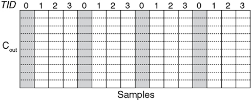
Figure 3. Threaded matrix multiplication. In this load-balanced example, four threads each calculate four samples, for a total of 16 output samples. The samples that thread 0 calculates are highlighted in gray.
The general form of this algorithm is demonstrated here:
where TID is a number indicating the thread number, or thread-ID (0 ≤ TID < numThreads), and numThreads is the total number of threads used, which is typically equal to the number of CPU cores.
In the previous example with 2 CPU cores and 120 samples, each thread would calculate the output for 60 samples, equally dividing the processing load and minimizing thread overhead. Using this paradigm, the load is balanced when the number of samples is a multiple of the number of cores, i.e., S = k × numThreads. This is illustrated by considering the case where instead of 2 cores, 8 cores are used to process 100 samples. Here, 4 threads process 12 samples, and 4 threads process 13 samples, resulting in an unequal load, the effect of which is multiplied for a large number of channels. For example, if there are 512 input and output channels, then 512 × 512, or 262,144, additional operations will be performed on the cores that run an extra iteration.
CUDA Spatial Filter
The NVIDIA CUDA system includes an implementation of Basic Linear Algebra Subprograms (BLAS) called CUBLAS, which provides a vector and matrix multiplication routines optimized for GPU execution (NVIDIA, 2008a
). The implementation details of the BLAS libraries are largely hidden to the user; however, v2.0 of the CUBLAS library incorporates methods presented in Volkov and Demmel (2008)
, in which the authors presented matrix–matrix multiply routines that run up to 60% faster that the v1.1 of CUBLAS. Depending on the matrix dimensions, it is possible to obtain performance close to the theoretical maximum capabilities of the GPU with the CUBLAS library.
Auto-Regressive Power Estimation Overview
BCI2000 uses an AR model to estimate the sensorimotor rhythm amplitudes for control. This model can be expressed as:

where Yt is the predicted signal at time t, a is a vector of p coefficients, and e is the prediction error. a is a vector of estimated filter coefficients for an all-pole model of order p, for which the power spectrum is found as:
The power P at a particular frequency ω is found using Eq. 4; note that it is theoretically possible to find the power at any arbitrary frequency and resolution, which is not possible with the FFT. Several methods exist for solving for the a coefficients; BCI2000 employs the Maximum Entropy (or Burg) Method, which is always guaranteed to produce a stable model (Cover and Thomas, 2006
; Fabiani et al., 2004
; Krusienski et al., 2006
).
BCI2000 calculates the power in adjacent bins of equal width, generally between 1 and 5 Hz for EEG, and larger for ECoG. Within each bin, the power is estimated at evenly spaced intervals and averaged. For example, a 2-Hz bin from 10–12 Hz with 11 evaluations would find the power in 0.2 Hz intervals (Eq. 4):
Thus, depending on the total frequency range and the bin width, each channel will have a number of binned power spectrum amplitudes, which are used as the control signal features in the subsequent BCI2000 signal processing steps.
The method for calculating the AR coefficients is briefly summarized in this paper. The details can be found in Press et al. (1999)
, and the source code is provided in the BCI2000 distribution. We did, however, implement a more efficient version of the algorithm based on Andersen (1978)
for all three computational methods (BCI2000, CPU-threaded, and CUDA), which provided performance gains of more than 30% for larger data sets.
Multi-Threaded (CPU) Auto-Regressive Power Estimation
The CPU-based multi-threaded algorithm is identical to that found in BCI2000 and in Press et al. (1999)
. Currently in BCI2000, the power is calculated for each channel sequentially in a loop, and does not take advantage of multi-core processors. Therefore, a parallel method was developed in which the power is estimated for a group of channels in individual threads, so that for T threads and C channels, each thread calculates the power for C/T channels. For example, for C = 20 and T = 4, thread 0 will calculate channels 1, 5, 9, 13, and 17, thread 1 will calculate 2, 6, 10, 14, and 18, etc. In the case that C is not a multiple of T, some threads will calculate the power for one fewer channel, resulting in an imbalanced thread load.
CUDA Auto-Regressive Power Estimation
The CUDA AR power estimation procedure is divided into two distinct steps, which involves first estimating the AR model coefficients, and then finding the binned average power. The theory behind this algorithm is beyond the scope of this paper; discussions of the algorithm can be found in Chen (1988)
, Makhoul (1975)
, and Press et al. (1999)
. The general concepts for implementing the AR algorithm on the GPU are presented here.
The form of the power spectrum is given in Eq. 4, in which ap is estimated using forward and backward recursion. Given the series xt, the linear prediction estimate  and error et are:
and error et are:

Then, the forward and backward prediction errors at step p are defined as:


The model is guaranteed to be stable and have minimum phase by minimizing the average prediction power of the forward and backward estimates (Pf,p and Pb,p, respectively):


The prediction error is minimized by solving δPp/δap = 0 for all values of p, giving:
With each iteration from 1 to p, ap is recalculated based on the forward and backward prediction errors at each step.
The original algorithm intended to execute on a single processor simply solved for the coefficients iteratively using for-loops, e.g., for the k-th iteration, the numerator and the denominator of Eq. 13 would be found as:
However, as mentioned previously, it is inefficient to execute loops like this on the GPU. Therefore, the reduction method is employed in instances such as this to solve for the numerator and denominator, so that each thread in a block calculates some small portion of the sum instead of the entire sum. To do so, assume that the
ef and eb are of length N − k, and that a scratch buffer named buf is available in shared memory with T elements, where T is the number of available threads and is a power of 2. Then, to find the numerator, for example, each thread, having a thread ID 0 ≤ TID < T, executes the following code:
Using this reduction framework, all of the summations and iterations in the original Burg AR algorithm were ported to take advantage of 100 s of threads running simultaneously. In fact, the second half of the above code in which the elements of
buf are summed works for any such loop, and was therefore implemented as a generic function used repeatedly throughout the algorithm. It should also be noted that this section is not completely optimized for the device architecture, but is instead presented for clarity of the concept. A more efficient method is used in the actual source code, and is described in the Reduction example in the NVIDIA CUDA SDK.The program was configured so that a single block calculates a single channel, regardless of the number of channels. For the benchmarking procedure, the block used either 64 or 128 threads, depending on which produced the faster time (see the Results for details on this procedure). The algorithm uses several shared memory buffers to hold the forward and backwards prediction errors and other temporary buffers, the sizes of which are dependent on the number of samples processed and the model order. The total shared memory required for a single channel is equal to [S × 3 × 4 + (M + 1) × 2 × 4 + 72] bytes, where S is the number of samples and M is the model order. With a total of 16384 bytes of shared memory per block, if an order 30 model is used, then at most 1338 samples can be processed at a time. While somewhat limiting, in practice this is equivalent to 278.75 ms of data sampled at 4800 Hz, which is acceptable for most applications.
Once the ap coefficients are found for each channel, the second half of the AR algorithm uses them to calculate the power amplitude at specific frequencies. In this case, the GPU computational grid is configured in a two-dimensional array of blocks, where the rows correspond to each channel, and the columns correspond to the frequency bins for each channel. Within a block, the power in each bin is calculated by E threads that evaluate the power spectrum at E equally spaced locations, depending on the bin width and the number of evaluations per bin. That is, each thread solves Eq. 4 for unique values of ω.
When all values of ω in a bin are evaluated, they are summed using reduction, and divided by the number of evaluations per bin to find the average. This final values for all channels and bins are then transferred back to global device memory on the GPU, which is then transferred from the GPU to the CPU, thus completing the power calculation.
Experimental Procedure
In a typical experiment, BCI2000 reads a block of neural data from the amplifier, and first spatially filters the signal. The results of the spatial filter are concatenated to the end of a buffer containing the values of the previous several blocks. Finally, the power spectral estimate is calculated for the entire buffer. For example, the duration of a sample block might be 50 ms with a buffer that contains five blocks of data (the current block plus the four previous blocks) for a total of 250 ms. The tests performed in this study were designed to mimic realistic testing conditions; therefore, the spatial filter is tested on 50 ms blocks of simulated neural data (i.e., a 10 Hz, 10 μV signal added to 2 μV white noise with a random distribution) for three sampling rates (512, 2400, and 4800 Hz), which is equivalent to sample sizes of approximately 25, 120, and 240 samples respectively. Similarly, since the power is found over 250 ms, the timing was found for sample sizes of 125, 600, and 1200 samples (250 ms at 512, 2400, and 4800 Hz, respectively). A total of 19 different channel counts were tested, shown in Table 1
. During an actual experiment, the spatial filter may only produce a subset of the output channels, e.g., only 8 channels out of 128 with relevant information might be spatially filtered (although all 128 channels are used for the calculation of each output channel), and then passed to the power estimation. However, in all test cases the number of output channels from the spatial filter equaled the number of input channels, to estimate the maximum expected processing time for a given configuration. Every combination of channel count (19) and sample count (3) was tested, for a total of 57 tests, and each test was repeated 100 times.
First, each test was performed using the original single-threaded algorithms, the multi-threaded algorithms, and the CUDA algorithms. An event timer with sub-ms resolution is provided by the CUDA library for benchmarking purposes, which was started at the beginning of each iteration of each test. This time includes the data transfer to and from the video card for the CUDA test, which can be a significant portion of the overall processing time. For each number of input samples, the processing times were compared for the three computational methods. The speedup of each algorithm was then found and compared across the number of samples by finding the ratio of the processing times for two computational methods, including single-threaded and multi-threaded, single-threaded and CUDA, and multi-threaded and CUDA. Therefore, if the ratio between two computational methods was >1, then second algorithm was faster.
It is possible to select the number of threads the GPU uses for the AR power estimate. Therefore, different numbers of threads were tested for different numbers of input samples to determine whether more threads is always better, as might be expected. The number of threads tested was always a power of 2, starting at 16 threads up to 256 (24 through 28). The number of samples tested ranged from 100 to 1200, in 100 sample increments. Only inputs of 128 channels were tested. The minimum processing time for each sample count was found for each number of threads.
Finally, the total overall combined processing times were measured. For the CPU multi-threaded and single-threaded methods, this was simply the sum of the spatial filter and power estimation times. For the CUDA method, two conditions were tested to determine the effects of data transfer to and from the device. In Figure 4
, A shows the data path in which the GPU calculates the spatial filter, transfers the data to the CPU then back to the GPU to calculate the power. The total processing time for this path includes two transfers to the GPU and two transfers from the GPU, and is the sum of (t1a − t0) and (t3a − t2a). Conversely, in B, the data remains on the GPU following the spatial filter, and is passed directly to the power estimate; the processing time here is found as (t1b − t0). The memory address of the spatial filter result persists in global GPU memory even after the function finishes; therefore, the memory location can be passed to the power estimation function without the need to transfer the data back and forth in between functions.
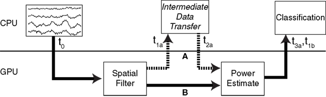
Figure 4. Two possible data transfer paths. (A) Following the spatial filter, data is transferred to the CPU before being transferred back to the GPU for the power estimate. This incurs an additional overhead that can contribute significantly to the overall processing time. (B) The data remains on the video card after spatial filtering for the power estimation routine.
The total processing times and processing speedup were then compared as before. Additionally, the speedup for the total CUDA processing time with and without intermediate data transfer was compared. The mean processing times (μ), the standard deviation (σ), coefficient of variation (100 × σ/μ), and maximum processing times were found for each computational method to determine how consistent the timing of each was over 1000 iterations. The methods developed were tested on the Windows XP, Mac OS X, and Linux Ubuntu 8.10 operating systems; however, the results given are for those obtained with Windows, and any significant OS-dependent differences are noted as appropriate.
Spatial Filter
The spatial filtering times in μs are plotted in Figure 5
A, and the ratios of processing times for each method are shown in Figure 5
B for the three sample lengths tested. Regardless of the number of samples, for a small number of channels the single-threaded method out-performs the multi-threaded and CUDA methods. The CUDA spatial filter performs better than the single-threaded method after between 8 and 48 channels, depending on the number of samples processed. When 1000 channels and 240 samples were tested, CUDA performs more than 100 times faster (8 ms vs. 807 ms) than the single-threaded method.
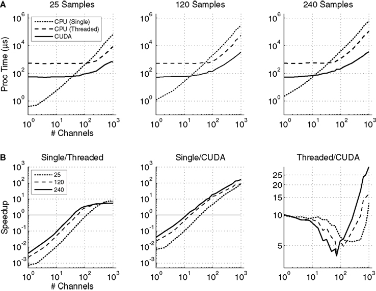
Figure 5. (A) The processing times for the single-threaded (dotted line), multi-threaded (dashed line), and GPU (solid line) matrix multiplication algorithms for time-series data with lengths of 25, 120, and 240 samples, which are equivalent to 50 ms of data at 512, 2400, and 4800 Hz, respectively. (B) The ratios of matrix-multiplication processing times for single-threaded to multi-threaded, single-threaded to CUDA, and multi-threaded to CUDA implementations. The results for input matrices with 25 (dotted line), 120 (dashed line), and 240 (solid line) samples are shown. A value exceeding 1 indicates that the processing time for the first implementation in the ratio exceeds that of the second implementation (e.g., if Single/Threaded >1, then the threaded version is faster). The spatial filter is a square matrix with the number of rows and columns each equal to the number of channels.
The CUDA version also out-performs the multi-threaded version by at least 5×. For channel counts <8, the GPU performs about 10× faster than the CPU. However, between 8 and 100 channels, the CPU performance increases to only 5× slower than GPU performance. Then, once the channel count surpasses 100 up to 1000, the GPU performance jumps up to 25× faster than the CPU for 240 samples, and up to 15× for 120 and 25 samples.
Auto-Regressive Power Estimation
Figure 6
A shows the AR power estimation processing times in μs vs. the number of channels for 125, 600, and 1200 samples, and for the three computational methods. Figure 6
B shows the ratio of processing times for the three methods.
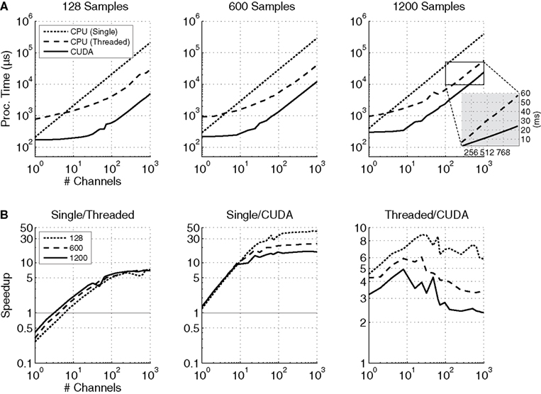
Figure 6. (A) The processing times for the single-threaded (dotted line), the multi-threaded (dashed line), and CUDA (solid line) auto-regressive power estimation algorithms for time-series data with lengths of 128, 600, and 1200 samples. For 1200 samples, the threaded processing time is 56 ms, while the CUDA processing time is 24.21 ms, as shown in the blow-up graph. (B) The ratios of power estimation processing times for single-threaded and multi-threaded, single-threaded and CUDA, and multi-threaded and CUDA implementations. The results for input matrices with 128 (dotted line), 600 (dashed line), and 1200 (solid line) samples are shown. A value exceeding 1 indicates that the processing time for the first implementation in the ratio exceeds that of the second implementation (e.g., if Single/Threaded >1, then the threaded version is faster).
The multi-threaded CPU implementation out-performs the single-threaded implementation when the number of channels is equal to or greater than 3, 4, or 6 when 1200, 600, or 125 samples are processed, respectively. The maximum speedup (7×) is approximately equal to the number of cores (8); however, the performance gain will never equal 8× due to the overhead associated with threading.
Larger performance gains are seen with the CUDA implementation. Even when only a single channel is processed, the GPU method is approximately equal to the single-thread performance (190 μs vs. 210 μs, respectively for 125 samples processed). When 1000 channels are processed, the performance gain is between 12 and 34 times, depending on the number of samples processed.
When compared to multi-threaded CPU performance, the CUDA method is generally at least twice as fast. However, there is a performance plateau at about 2× when more than 128 channels and 1200 samples are processed; when 1000 channels and 1200 samples are processed, the CUDA processing time is 27.51 ms, while the multi-threaded time is 56 ms. This relationship holds as more channels are added; e.g., when 2000 channels are processed (not shown), the processing times are 54 and 115 ms, respectively, an increase of more than 2.1×.
This performance can be partially explained by Figures 7
A,B, which show the CUDA processing times vs. the number of threads for different numbers of samples processed, from 100 to 1200 in 100-sample increments. Panel A shows that for smaller numbers of samples processed (100–500 samples), processing using 64 threads is more efficient than 128 or 256 threads, while for a larger number of samples (600–1200), 128 threads works fastest. In no case was 256 threads fastest.
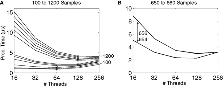
Figure 7. (A) Processing time using different numbers of threads with CUDA for different data lengths from 100 to 1200, in 100-sample increments, and 128 input channels. A * indicates a minimum processing time. For shorter data segments (e.g., 100–400 samples), a lower number of threads is more efficient, while for longer data segments (e.g., > 500 samples), an increased number of threads results in a faster processing time. Up to 256 threads were tested, but in no cases was 256 threads the most efficient, showing that more threads does not necessarily guarantee better performance. (B) When increasing from 654 to 656 processed samples, there is a large jump in the processing time, resulting from the way in which the data is loaded into memory on the GPU.
Of particular importance is the large jump in time occurring between 500 and 600 samples; this jump occurs when increasing the sample count from 654 to 656, as shown in Figure 7
B. This sudden decrease in performance occurs due to the algorithm design and how it interacts with the underlying hardware. As discussed previously, the power is calculated on a channel-by-channel basis, in which each channel is assigned to a processing block. A block runs on an individual processor on the GPU, which has up to 16384 bytes of shared memory available. If the block uses less than half of the shared memory available (8192 bytes), then the memory transfers for multiple blocks on a single processor can be hidden by the GPU; that is, while one block is being processed, memory for the other block can be pre-loaded into shared memory. However, if more than half of the shared memory is used by a single block, then the shared memory cannot be pre-loaded, and the processing time will increase. Each channel requires [S × 3 × 4 + (M + 1) × 2 × 4 + 72] bytes of memory, where S is the number of samples and M is the model order. Therefore, for S = 654, M = 30, the shared memory required is 8172 bytes, but if S = 654, M = 30, then 8196 bytes of shared memory are required, thus reducing processing efficiency.
Total Speedup
The total processing times and speedup for both the spatial filter and power estimations are shown in Figure 8
. In these plots, the spatial filter processed 1/5 of the number of samples shown, e.g., when 125 samples are shown, then the spatial filter actually processed 25. This simulates the real-time BCI procedure, in which the spatial filter is updated with every sample block (50 ms), and the AR estimate processes five blocks at a time (250 ms).
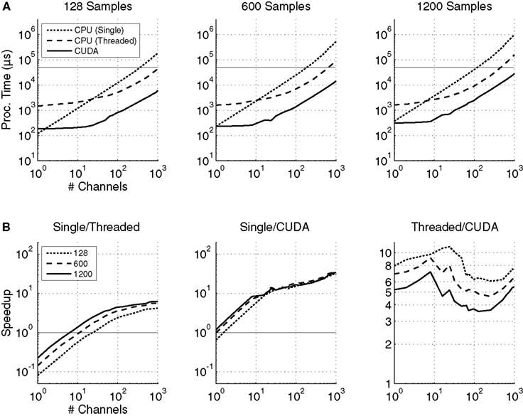
Figure 8. (A) The combined spatial filtering and power estimation processing times for single-threaded, threaded, and CUDA based implementations. The spatial filter processed one-fifth of the samples shown (i.e., 25, 120, and 240 samples), while the AR algorithm estimated the power for the total length of data. The solid horizontal line is at 50 ms, indicating the real-time performance threshold. (B) The ratios of combined spatial filtering and power estimation processing times for single-threaded and threaded, single-threaded and CUDA, and threaded and CUDA implementations. A value exceeding 1 indicates that the processing time for the first implementation in the ratio exceeds that of the second implementation (e.g., if Single/Threaded >1, then the threaded version is faster).
For the single and multi-threaded computational methods, the total time is simply the sum of the processing times for each individual step. For the CUDA method, summing the two values produces an inaccurate estimate of the processing time, since it would include the time required to transfer the result of the matrix multiplication from the GPU to the CPU, then transfer it back to the card for the AR algorithm to operate on it. Therefore, the CUDA processing time is the correct estimate that does not include the intermediate data transfer. Figure 9
shows the differences between the CUDA processing times when the data transfer is included; generally, the speedup if the extra transfer is removed is between 1.25 and 2 times faster.
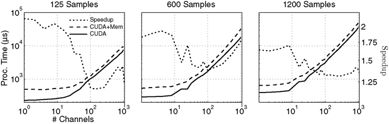
Figure 9. Comparison of processing times in μs for combined spatial filter and AR power estimates done with data transfer to and from the video card in between processing steps (CUDA + Mem), and without data transfer. The overall speedup by removing the intermediate data transfer is shown on the Y-axis, and is generally 1.5 to 2 times faster. The graphs show the processing times for data lengths of 125, 600, and 1200 samples, from left to right.
Figure 8
A shows the total processing time for the three methods. As expected, the CUDA implementation outperforms the single-threaded implementation by nearly two orders of magnitude for large numbers of channels. The total processing time for 1000 channels with 1200 samples was 32 ms, compared to 933 ms for the single-threaded version and 163 ms for the multi-threaded version.
The consistency of the timing is also an important consideration. Table 2
shows some of the representative timing statistics for each method. The mean (μ), standard deviation (σ), coefficient of variation (Cv), and the overall maximum times are shown for several channel–sample count combinations. In a timing-critical application such as a BCI, in which it is necessary to process all of the data within a given time period (i.e., the sample block size), it is crucial not just that the mean processing time is less than the critical-period, but that all processing times are less than the period. Therefore, the standard deviation provides a measure of how much the processing time will vary from block to block. Additionally, as the number of processed elements increases, it is likely that the variability in the processing times will increase as well, at least on the CPU; Cv is the ratio σ/μ, and provides a method of ensuring that the processing time variability scales well with the mean processing times.
In Table 2
, Cv is the largest for the multi-threaded methods, which is not unexpected, since Windows runs many processes unrelated to the signal processing task concurrently. Therefore, if all eight cores are used for calculating the power, there may be a delay prior to a particular thread beginning, while the operating system finished another task. In contrast, the single-thread version only requires a single core, and is therefore less likely to be pre-empted, resulting in less variation, even for long processing times.
For small processing times, CUDA has what seems to be a large Cv. In fact, this is primarily due to a small μ, which can skew the Cv values. The timing variability remained small for small data sets; as the processing time increased, Cv decreased, indicating that the processing times are very consistent even for large data sets. This corresponds with the fact that the OS does not preempt the GPU as it does the CPU, and therefore the GPU can devote all of its resources to the task.
Implantable neuroprosthetic electrode technology is continuing to evolve by adding more recording sites and transmitting at higher bandwidths, while increasingly complex neural feature extraction and classification algorithms are developed to improve performance. However, the current generation of computer hardware is already being stretched to its limits by relatively low channel counts. If real-time performance is defined as the ability to update the feedback device at least every 50 ms (Schalk et al., 2004
), then the results in this study show that the current (single-threaded) version of the signal processing routine is unable keep up when more than 100 channels are used.
Additionally, there are other system latencies present that will also contribute to the overall time required to update the display, including the time required to transfer data from the amplifier to the PC, additional signal processing latencies not addressed here (e.g., collision detection in the cursor movement task), and the output latency, which is the delay between when an output command is issued and when it actually happens. This depends on the operating system, the video card (for video), and the monitor type itself. In another study, methods were devised to measure the latencies at each step in the signal processing chain in order to model the expected latencies for a given task configuration (Wilson et al., submitted
). Results from those tests indicate that the current single-threaded version of BCI2000 would be able to process approximately 36 channels of 2400 Hz data every 50 ms, including all other aforementioned latencies. When the tests were run using the CPU multi-threaded version, up to 220 channels were processed in under 50 ms, while the CUDA version supported more than 500 channels.
In the tests shown here, the CPU-based multi-threaded algorithms significantly outperform the single-threaded versions, begging the question of whether the work required to port existing programs to run on the GPU is worth the benefit. One of the benefits of using a video card for computation is that it is relatively cheap and simple to upgrade the video card when new versions are released or if more performance is required. Conversely, it requires much more work to upgrade the CPU; the motherboard and RAM will likely need to be replaced, and the operating system may need to be re-installed or re-activated as well if Windows detects new hardware. Finally, the processing power of video cards is progressing at a much faster rate than CPUs. There are currently no consumer-level computers commercially available with more than 8 cores, while the new NVIDIA Tesla systems have more than 940 cores, compared to <100 cores a year ago. Other current NVIDIA graphics cards with 240 cores and 896 MB RAM are available for approximately $200 (the GTX 275). This trend is likely to continue, increasing the benefit of using GPU computation. Another benefit of using the GPU for processing is that it obviates many of the benefits of a real-time Linux system; since all of the processing is done on the GPU and not the CPU, it is impossible for the OS to interrupt or interfere with processing, as demonstrated in Table 2
. Even when large amounts of data were processed, the GPU processing times have a very small standard deviation compared to the single or multi-threaded CPU implementations. Therefore, it is feasible to use a non-real-time OS, such as Windows, even for time-critical applications.
Another consideration is the availability of powerful graphics cards that are becoming available in portable laptop computers. For example, the 2009 models of the Macbook Pro laptops from Apple have two NVIDIA cards installed. One of the cards is intended for longer battery life and therefore has reduced processing power, while the other is intended for graphics-intensive applications, and could be considered a desktop-replacement video card. It is therefore possible to use the second card for processing data, while the first only has to handle the display updates. In testing these new laptops, the processing power of graphics card was found comparable to the 8-core Mac Pro using the CPU (data not shown). For example, it required 154.34 ms to process 1000 channels sampled at 4800 Hz in 250 ms segments on the new Macbook Pro graphics card, whereas the Mac Pro took 162.53 ms to process the same data on the CPU. The implication is that fully portable BCI systems with high-bandwidth, high-channel count data are available in current-generation laptops, which are significantly less expensive than a stationary eight-core workstation, yet just as capable of processing large amounts of data. As discussed, this trend is likely to continue in the foreseeable future: the next generations of laptops will contain increasingly powerful video cards, while simultaneously seeing little relative increases in CPU power.
Finally, these processing methods introduce the possibility of performing BCI algorithms which were once considered too complex or intensive for real-time calculation, but otherwise are very capable offline analysis tools (Chen et al., 2008
; Delorme and Makeig, 2004
; Hu et al., 2005
; Kim and Kim, 2003
; Laubach, 2004
; Letelier and Weber, 2000
) . Feature extraction methods that include neural networks, wavelet analysis, and independent or principal component analysis could possibly be used in a real-time environment, although these were not addressed in this study. Furthermore, other types of data, such as neural spike data recorded from microelectrodes (Hatsopoulos et al., 2005
; Kipke et al., 2003
) or high-channel count microelectrode arrays with neural cell cultures (Colicos and Syed, 2006
), could be processed on the computer, instead of on an expensive dedicated hardware system.
In conclusion, the results from this study show that massively parallel processing architectures currently available are capable of improving the performance of BCI system by at least two orders of magnitude with the algorithms tested. Other neural feature extraction methods will also undoubtedly benefit as well, and because video cards are easily upgraded (at least in desktop systems), it is straightforward to scale processing needs for the desired applications.
The authors declare that the research was conducted in the absence of any commercial or financial relationships that could be construed as a potential conflict of interest.
The authors would like to thank Profs. Dan Negrut and Erick Oberstar in the Mechanical Engineering Department at the University of Wisconsin for advice on programming with CUDA, and Dr Gerwin Schalk at the Wadsworth Center (Albany, NY, USA).
NVIDIA (2009). NVIDIA GeForce 8 Series. URL: http://www.nvidia.com/page/geforce8.html