Multivariate tempered stable model with long-range dependence and time-varying volatility

1. Introduction

The long-range dependence, fat-tail property, and volatility clustering effect are important issues for modeling high-frequency return time series in finance. The fractional Brownian motion introduced by Mandelbrot and Ness [1] can explain short-range or long-range dependence but it cannot explain the volatility clustering effect. The volatility clustering effect can be captured by the autoregressive conditional heteroskedastic (ARCH) and the generalized ARCH (GARCH) models formulated by Engle [2] and Bollerslev [3], respectively. However, GARCH models based on the normal distribution have not performed well in explaining high-frequency data analysis (see [4] and [5]), since the normal distribution does not capture the fat-tail property in the empirical innovation. To capture the fat-tail property in high-frequency return data, [5] suggested the univariate ARMA-GARCH model with tempered stable innovations without considering long-range dependence. The long-range dependence in high-frequency data is empirically reported in Sun et al. [6]. Sun et al. [4] provide a univariate model having long-range dependence, fat-tail property, and volatility clustering by taking the ARMA-GARCH model with fractional stable noise residuals exhibits, and show that the model has superior performance in high-frequency returns.

In this paper, a new multivariate market model that describes the long-range dependence, fat-tail property, and volatility clustering effect is developed. The new market model is constructed by taking the fractional tempered stable innovations on the multivariate ARMA-GARCH model. Univariate fractional tempered stable process was defined by the stochastic integral for the Volterra kernel in Houdre and Kawai [7] based on subclasses of Rosinski's tempered stable processes [8]. In order to construct multivariate model, we would better use normal tempered stable (NTS) process rather than Rosinski's tempered stable processes, since the NTS process is defined by the time-changed Brownian motion, and hence we can easily obtain a multivariate model which allows fatter tails than the multivariate Gaussian distribution and an asymmetric dependence structure. The NTS process has been discussed in many literatures including [9–12], and [13]. Although NTS is not included in Rosinski's tempered stable processes (see [14]), the fractional NTS process is redefined in this paper. The fractional NTS process is a multivariate process having the long-range dependence in time and asymmetric dependence between elements¹.

To verify the performance of the new model, empirical illustration is provided using high-frequency stock return data. Useful simulation and parameter estimation methods are provided, and the goodness-of-fit tests are performed for the estimated parameters. The long-range dependence and fat-tail property of the high frequency stock return data are observed by this investigation.

To apply the new model for the financial risk management and portfolio management, portfolio value-at-risk (VaR), average VaR (AVaR), and portfolio optimization based on the new market model are discussed. VaR has a number of well-known limitations as a risk measure, nevertheless the VaR measure has been popularly used as a standard risk measure in the financial industry. The AVaR is the average of VaRs exceeding the VaR for a given confidence level² AVaR is a superior alternative to VaR because it is a coherent risk measure³. and it is consistent with preference relations of risk-averse investors (see [20]).

A major contribution to the portfolio theory is the mean-variance model presented by Markowitz [21]. The importance of the model cannot be overstated, but some of assumptions underlying the model have been challenged since its introduction. One of the assumptions is that asset returns follow a Gaussian (normal) distribution and another is that the variance is a measure of risk ignoring higher-order moments. In this paper, the portfolio optimization is discussed based on the Markowitz's theory, but the Gaussian assumption is replaced by the ARMA-GARCH model with fractional NTS innovations and the variance risk measure is superseded by VaR and AVaR risk measures.

The remainder of this paper is organized as follows. The NTS process is reviewed in Section 2. The definition of the multivariate fractional NTS process and its simulation method are presented in Sections 3, 4, respectively. Multivariate ARMA-GARCH model having long-range dependence is defined in Section 5 along with the empirical illustration. In Section 6, portfolio risk will be assessed and the optimal portfolio will be found based on the new ARMA-GARCH model using high-frequency market data. In Section 7, the principal findings are summarized. Volterra kernel is briefly reviewed in the appendix.

2. Normal Tempered Stable Process

In the remainder of this paper, we assume that N is a positive integer standing for the dimension and α ∈ (0, 2), θ > 0, β = (β₁, β₂, …, β_N)^T, γ = (γ₁, γ₂, …, γ_N)^T such that γ_n > 0 for n ∈ {1, 2, …, N}, and Σ = [σ_m,n]_{m,n∈{1, 2, …, N}} is a given correlation matrix such that σ_n,n = 1 for n ∈ {1, 2, …, N}. The pure jump Lévy process T = (T(t))_{t ≥ 0} whose characteristic function ϕ_T(t) is equal to

${\varphi }_{T(t)}(u)=\exp \left(\frac{{\theta }^{1-\frac{\alpha }{2}}t}{\Gamma \left(1-\frac{\alpha }{2}\right)}{\displaystyle {\int }_0^{\infty }(e^{iux}-1)}\frac{e^{-\theta x}}{x^{\alpha /2+1}}dx\right).$

is a subordinator and referred to as the tempered stable subordinator with parameters (α, θ). Solving the integration in the last Equation, we can obtain the following formula,

$\begin{array}{ll}{\varphi }_{T(t)}(u)=\exp \left(-\frac{2{\theta }^{1-\frac{\alpha }{2}}t}{\alpha }\left({(\theta -iu)}^{\frac{\alpha }{2}}-{\theta }^{\frac{\alpha }{2}}\right)\right).\hfill & (1)\hfill \end{array}$

Consider a N-dimensional Brownian motion B = (B(t))_{t ≥ 0} such that B(t) = (B₁(t), B₂(t), …, B_N(t))^T, and suppose that

$\text{cov}(B_m(t),B_n(t))={\sigma }_{m,n}t$

for all m, n ∈ {1, 2, …, N}.

Suppose T is independent of B. Consider a N-dimensional process Z = (Z(t))_{t ≥ 0} such that Z(t) = (Z₁(t), Z₂(t), …, Z_N(t))^T. For n ∈ {1, 2, …, N}, define (Z_n(t))_{t ≥ 0} by the time-changed Brownian motion as

$\begin{array}{ll}{Z}_n(t)={\beta }_n(T(t)-t)+{\gamma }_n{B}_n(T(t)).\hfill & (2)\hfill \end{array}$

Then the process Z is referred to as the N-dimensional NTS process with parameters (α, θ, β, γ, Σ) and we denote by Z~ NTS_N (α, θ, β, γ, Σ).

By composing characteristic functions of B(t) and T(t), we obtain the characteristic function of Z_n(t) as follows:

$\begin{array}{ll}\begin{array}{l}{\varphi }_{Z_n(t)}(u)= \\ \exp \left(-{\beta }_{n}uti-\frac{2{\theta }^{1-\frac{\alpha }{2}}}{\alpha }t\left({\left(\theta -i{\beta }_{n}u+\frac{{\gamma }_n^2{u}^2}{2}\right)}^{\frac{\alpha }{2}}-{\theta }^{\frac{\alpha }{2}}\right)\right)\text{}\text{}.\end{array}\hfill & (3)\hfill \end{array}$

The mean of Z_n(t) is equal to zero for n ∈ {1, 2, …, N}. Covariance between Z_m(t) and Z_n(t) is given by

$\begin{array}{ll}\text{cov}(Z_m(t),Z_n(t))=t{\gamma }_m{\gamma }_n{\sigma }_{m,n}+t{\beta }_m{\beta }_n\left(\frac{2-\alpha }{2\theta }\right)\hfill & (4)\hfill \end{array}$

for m, n ∈ {1, 2, …, N}. Moreover the variance of Z_n(t) is equal to

$\begin{array}{ll}\text{Var}(Z_n(t))=t\left({\gamma }_n^2+{\beta }_n^2\left(\frac{2-\alpha }{2\theta }\right)\right)\hfill & (5)\hfill \end{array}$

The linear combination of elements of Z is also NTS as follows.

Proposition 1. Let w = (w₁, w₂, …, w_N)^T ∈ ℝ^N, Z ~ NTS_N (α, θ, β, γ, Σ), and Y(t) = $Y(t)={\displaystyle {\sum }_{n=1}^N{w}_n}{Z}_n(t)$. Then (Y(t))_{t ≥ 0}~ NTS₁(α, θ, β, γ, 1), where

$\overline{\beta }={\displaystyle \sum _{n=1}^N{w}_n}{\beta }_n,\text{and }\overline{\gamma }=\sqrt{{\displaystyle \sum _{m=1}^N{\displaystyle \sum _{n=1}^N{w}_m}}{w}_n{\gamma }_m{\gamma }_n{\sigma }_{m,n}}.$

Proof. See [12].

If ${\gamma }_n=\sqrt{1-{\beta }_n^2\left(\frac{2-\alpha }{2\theta }\right)}$ and $\left|{\beta }_n\right|<\sqrt{\frac{2\theta }{2-\alpha }}$ for n ∈ {1, 2, …, N} then var(Z_n(t)) = t. In this case the process Z is referred to as the N-dimensional standard NTS process with parameters (α, θ, β, Σ) and denoted by Z ~ stdNTS_N (α, θ, β, Σ).

3. Fractional Normal Tempered Stable Process

Let K_H(t, s) be the Voltera kernel and Z ~ NTS_N (α, θ, β, γ, Σ). The N-dimensional fractional NTS (fNTS) process generated by Z is defined by the process of vector X = (X(t))_{t ≥ 0} with X(t) = (X₁(t), X₂(t), …, X_N(t))^T such that

$X_n(t)=\underset{\left|\right|P\left|\right|\to 0}{\lim }{\displaystyle \sum _{j=1}^M{K}_H}(t,t_{j-1})\left(Z_n(t_j)-Z_n(t_{j-1})\right)$

in distribution sense for n ∈ {1, 2, …, N}, where

$P:0=t_0<t_1<\cdots <t_M=t$

is a partition of the interval [0, t] and

$\left|\right|P\left|\right|=\max \{t_j-t_{j-1}|j=1,2,\cdots ,M\}.$

In this case we denote that $X_n(t)={\displaystyle {\int }_0^t{K}_H}(t,s)d{Z}_n(s)andX~fNT{S}_N(H,\alpha ,\theta ,\beta ,\gamma ,\Sigma )$. Since we have

$\begin{array}{l}E\left[\left(iu{\displaystyle \sum _{j=1}^M{K}_H}(t,t_{j-1})\left(Z_n(t_j)-Z_n(t_{j-1})\right)\right)\right]\\ ={\displaystyle \prod _{j=1}^{M}E}\left[\exp \left(iu{K}_H(t,t_{j-1})\left(Z_n(t_j)-Z_n(t_{j-1})\right)\right)\right]\\ ={\displaystyle \prod _{j=1}^M\exp }(\text{}-{\beta }_{n}ui{K}_H(t,t_{j-1})(t_j-t_{j-1})\\ -\frac{2{\theta }^{1-\frac{\alpha }{2}}}{\alpha }((\theta -i{\beta }_{n}u{K}_H(t,t_{j-1})\\ {+\frac{{\gamma }_n^2{u}^2{(K_H(t,t_{j-1}))}^2}{2})}^{\frac{\alpha }{2}}-{\theta }^{\frac{\alpha }{2}})(t_j-t_{j-1}))\\ =\exp (\text{}-{\beta }_{n}ui{\displaystyle \sum _{j=1}^M{K}_H}(t,t_{j-1})(t_j-t_{j-1})\\ -\frac{2{\theta }^{1-\frac{\alpha }{2}}}{\alpha }{\displaystyle \sum _{j=1}^M((\theta -i{\beta }_{n}u{K}_H(t,t_{j-1})}\\ +{\frac{{\gamma }_n^2{u}^2{(K_H(t,t_{j-1}))}^2}{2})}^{\frac{\alpha }{2}}-{\theta }^{\frac{\alpha }{2}})(t_j-t_{j-1})),\end{array}$

the characteristic function of X_n(t) is given by

$\begin{array}{l}{\varphi }_{X_n(t)}(u)\\ =\underset{\left|\right|P\left|\right|\to 0}{\lim }\exp (-{\beta }_{n}ui{\displaystyle \sum _{j=1}^M{K}_H}\left(t,t_{j-1}\right)\left(t_j-t_{j-1}\right)\\ -\frac{2{\theta }^{1-\frac{\alpha }{2}}}{\alpha }{\displaystyle \sum _{j=1}^M((\theta -i{\beta }_{n}u{K}_H(t,t_{j-1})}\\ +{\frac{{\gamma }_n^2{u}^2{(K_H(t,t_{j-1}))}^2}{2})}^{\frac{\alpha }{2}}-{\theta }^{\frac{\alpha }{2}})(t_j-t_{j-1}))\\ =\exp (\text{}-{\beta }_{n}ui{\displaystyle {\int }_0^t{K}_H}(t,s)ds\\ -\frac{2{\theta }^{1-\frac{\alpha }{2}}}{\alpha }{\displaystyle {\int }_0^t((\theta -i{\beta }_{n}u{K}_H(t,s)}\\ +{\frac{{\gamma }_n^2{u}^2{(K_H(t,s))}^2}{2})}^{\frac{\alpha }{2}}-{\theta }^{\frac{\alpha }{2}})ds).\end{array}$

Proposition 2. For n ∈ {1, 2, …, N}, the covariance between X_n(s) and X_n(t) is equal to

$\begin{array}{ll}\begin{array}{l}\text{cov}(X_n(s),X_n(t))\\ =\frac{1}{2}\left({\gamma }_n^2+{\beta }_n^2\left(\frac{2-\alpha }{2\theta }\right)\right)\left(t^{2H}+s^{2H}-|t-s{|}^{2H}\right), s,t>0.\end{array}\hfill & (6)\hfill \end{array}$

Proof. Let P be a partition such that

$\begin{array}{l}P: 0=t_0<t_1<\cdots <t_{M-1}<t_M\\ =s\wedge t<t_{M+1}<\cdots <t_{M^{*}}=s\vee t.\end{array}$

Then we have

$\begin{array}{l}\mathrm{cov}(X_n(s),X_n(t))=E[X_n(s)X_n(t)]\\ =\underset{\left|\right|P\left|\right|\to 0}{\lim }E[{\displaystyle \sum _{j=1}^M{K}_H}(s,t_{j-1})\left(Z_n(t_j)2pt-Z_n(t_{j-1})\right)\\ {\displaystyle \sum _{k=1}^{M^{*}}{K}_H}(t,t_{k-1})\left(Z_n(t_k)2pt-Z_n(t_{k-1})\right)]\\ =\underset{\left|\right|P\left|\right|\to 0}{\lim }{\displaystyle \sum _{j=1}^M{\displaystyle \sum _{k=1}^{M^{*}}{K}_H}}(s,t_{j-1})K_H(t,t_{k-1})\\ E\left[\left(Z_n(t_j)-Z_n(t_{j-1})\right)\left(Z_n(t_k)-Z_n(t_{k-1})\right)\right]\end{array}$

By the property of the NTS process Z_n, we have

$\begin{array}{l}E\left[\left(Z_n(t_j)-Z_n(t_{j-1})\right)\left(Z_n(t_k)-Z_n(t_{k-1})\right)\right]\\ =\{\begin{array}{ll}(t_j-t_{j-1})Var(Z_n(1))\hfill & \text{ if }j=k\hfill \\ 0\hfill & \text{ if }j\ne k\hfill \end{array}\end{array}$

Hence, we obtain

$\begin{array}{l}\mathrm{cov}(X_n(s),X_n(t))=\underset{\left|\right|P\left|\right|\to 0}{\lim }{\displaystyle \sum _{j=1}^M{K}_H}(s,t_{j-1})K_H(t,t_{j-1})\\ (t_j-t_{j-1})Var(Z_n(1))\\ =Var(Z_n(1)){\displaystyle {\int }_0^{s\wedge t}{K}_H}(s,u)K_H(t,u)du.\end{array}$

Hence we obtain Equation (6) by Equation (5) and Equation (21) in Appendix.

Proposition 3. For m, n ∈ {1, 2, …, N}, the covariance between X_m(t) and X_n(t) is equal to

$\begin{array}{cc}\mathrm{cov}(X_m(t),X_n(t))=t^{2H}\left({\sigma }_{m,n}{\gamma }_m{\gamma }_n+{\beta }_m{\beta }_n\left(\frac{2-\alpha }{2\theta }\right)\right),t>0.& (7)\end{array}$

Proof. Let P be a partition such that

$P:0=t_0<t_1<\cdots <t_{M-1}<t_M=t.$

We have

$\begin{array}{l}\mathrm{cov}(X_m(t),X_n(t))=E[X_m(t)X_n(t)]\\ =\underset{\left|\right|P\left|\right|\to 0}{\lim }E[{\displaystyle \sum _{j=1}^M{K}_H}(t,t_{j-1})\left(Z_m(t_j)-Z_m(t_{j-1})\right)\\ {\displaystyle \sum _{k=1}^M{K}_H}(t,t_{k-1})\left(Z_n(t_k)-Z_n(t_{k-1})\right)]\\ =\underset{\left|\right|P\left|\right|\to 0}{\lim }{\displaystyle \sum _{j=1}^M{\displaystyle \sum _{k=1}^M{K}_H}}(t,t_{j-1})K_H(t,t_{k-1})\\ E\left[\left(Z_m(t_j)-Z_m(t_{j-1})\right)\left(Z_n(t_k)-Z_n(t_{k-1})\right)\right]\end{array}$

By the property of the NTS process Z_n, we have

$\begin{array}{l}E\left[\left(Z_m(t_j)-Z_m(t_{j-1})\right)\left(Z_n(t_k)-Z_n(t_{k-1})\right)\right]\\ =\{\begin{array}{ll}(t_j-t_{j-1})\mathrm{cov}(Z_m(1),Z_n(1))\hfill & \text{ if }j=k\hfill \\ 0\hfill & \text{ if }j\ne k\hfill \end{array}\end{array}$

Hence, we obtain

$\mathrm{cov}(X_m(t),X_n(t))=\mathrm{cov}(Z_m(1),Z_n(1)){\displaystyle {\int }_0^t(K_H(}t,u){)}^{2}du.$

Hence we obtain Equation (7) by Equation (4) and Equation (22) in Appendix.

For a given stochastic process Y = (Y(t))_{t ≥ 0}, the summation

${\displaystyle \sum _{j=1}^{\infty }E}[(Y(1)-Y(0))(Y(j+1)-Y(j))]$

diverges, then we say that Y exhibits long-range dependence (See [22]). By Proposition 2 and L'Hopital's rule, we have

$\begin{array}{l}E[X_n(1)(X_n(j+1)-X_n(j))]\\ =\frac{v}{2}\left({(j+1)}^{2H}-2j^{2H}+{(j-1)}^{2H}\right)\\ =\frac{v}{2}{j}^{2H-2}\left(j^2\left({\left(1+\frac{1}{j}\right)}^{2H}-2+{\left(1-\frac{1}{j}\right)}^{2H}\right)\right)\\ \to vH(2H-1)j^{2H-2}\text{ as }j\to \infty ,\end{array}$

where $v=\left({\gamma }_n^2+{\beta }_n^2\left(\frac{2-\alpha }{2\theta }\right)\right)$. Hence, ${\displaystyle {\sum }_{j=1}^{\infty }E}[X_n(1)(X_n(j+1)-X_n(j))]$ diverges, i.e., the process (X_n(t))_{t ≥ 0} has long-range dependence, when ½ < H < 1.

Since the NTS has an asymmetric dependence structure, X has also asymmetric dependence. By Proposition 1, we can prove the following proposition.

Proposition 4. Let w = (w₁, w₂, …, w_N)^T ∈ ℝ^N, X ~ fNTS_N (H, α, θ, β, γ, Σ), and $Y(t)={\displaystyle {\sum }_{n=1}^N{w}_n}{X}_n(t)$. Then (Y(t))_{t ≥ 0} ~ fNTS₁(H, α, θ, β, γ, 1), where

$\overline{\beta }={\displaystyle \sum _{n=1}^N{w}_n}{\beta }_n,\text{and }\overline{\gamma }=\sqrt{{\displaystyle \sum _{m=1}^N{\displaystyle \sum _{n=1}^N{w}_m}}{w}_n{\gamma }_m{\gamma }_n{\sigma }_{m,n}}.$

When Z ~ stdNTS_N (α, θ, β, Σ), the multivariate fractional NTS process X generated by Z is referred to as the fractional standard NTS process, and we denote that X ~ fstdNTS_N (H, α, θ, β, Σ). In this case, we have

$\begin{array}{cc}\mathrm{cov}(X_n(s),X_n(t))=\frac{1}{2}\left(t^{2H}+s^{2H}-|t-s{|}^{2H}\right), s,t>0.& (8)\end{array}$

and

$\begin{array}{cc}\begin{array}{l}\mathrm{cov}(X_m(t),X_n(t))\\ =t^{2H}({\sigma }_{m,n}\sqrt{1-{\beta }_m^2\left(\frac{2-\alpha }{2\theta }\right)}\sqrt{1-{\beta }_n^2\left(\frac{2-\alpha }{2\theta }\right)} \\ +{\beta }_m{\beta }_n\left(\frac{2-\alpha }{2\theta }\right)), t>0.\end{array}& (9)\end{array}$

By Proposition 4, we can prove the following corollary.

Corollary 5. Let w = (w₁, w₂, …, w_N)^T ∈ ℝ^N, X ~ fstdNTS_N (H, α, θ, β, Σ), and $Y(t)={\displaystyle {\sum }_{n=1}^N{w}_n}{X}_n(t)$. Then (Y(t))_{t ≥ 0} ~ fNTS₁(H, α, θ, β, γ, 1), where

$\overline{\beta }={\displaystyle \sum _{n=1}^N{w}_n}{\beta }_n,$

and

$\overline{\gamma }=\sqrt{{\displaystyle \sum _{m=1}^N{\displaystyle \sum _{n=1}^N{w}_m}}{w}_n{\sigma }_{m,n}\sqrt{1-{\beta }_m^2\left(\frac{2-\alpha }{2\theta }\right)}\sqrt{1-{\beta }_n^2\left(\frac{2-\alpha }{2\theta }\right)}}.$

4. Simulation

In this section, a numerical method is provided to generate the sample path for the multivariate fractional normal tempered stable process. By Theorem 5.3 (i) in Rosiński [8]⁴, we obtain series representation for the tempered stable subordinator T as follows:

$$\begin{array}{cc}T(t)=\underset{M\to \infty }{\lim }{\displaystyle \sum _{j=1}^M{1}_{(0,t)}}({\tau }_j)\left({\left(\frac{\alpha {\xi }_j\Gamma \left(-\frac{\alpha }{2}\right)}{2{\theta }^{1-\frac{\alpha }{2}}\mathcal{T}}\right)}^{-\frac{2}{\alpha }}\wedge \frac{e_j{u}_j^{\frac{2}{\alpha }}}{\theta }\right),t\in [0,\mathcal{T}],& (10)\end{array}$$

where

• {u_j} is an iid sequence of random variables on (0, 1),

• {e_j} and {e′_j} are an iid sequence of exponential random variables with parameter 1,

• ξ_j = e′₁ + e′₂ + … + e′_j,

• {τ_j} be an independent and identically distributed uniform random variable in [0, ], where > 0 is fixed.

• and assume that {u_j}, {e_j}, {e′_j} and {τ_i} are independent.

Let L_Σ be the lower triangular matrix obtained by the Cholesky decomposition for Σ with Σ = L_ΣL^T_Σ, where Σ is the correlation matrix in Equation (2). Then we have B(t) = L_Σ B(t) where B(t) = (B₁(t), B₂(t), …, B_N(t))^T is a mutually independent vector of Brownian motions.

Sample path of Z ~ NTS_N (α, θ, β, γ, Σ) is generated as follows. For a given partition {t₀, t₁, …, t_M} of the interval [0, ] with t₀ = 0, t_M = and t_j < t_k for j < k, we have

${\overline{B}}_n(T(t_j))-{\overline{B}}_n(T(t_{j-1}))=\sqrt{T(t_j)-T(t_{j-1})}{ϵ}_{j,n},n\in \{1,2,\cdots ,N\}$

where ϵ_j,n ~ N(0, 1). Therefore, we have

$\begin{array}{cc}Z(t_k)=(T(t_k)-t_k)\beta +\text{diag}(\gamma ){\displaystyle \sum _{j=1}^k\sqrt{T(t_j)-T(t_{j-1})}}{L}_{\Sigma }{ϵ}_j,& (11)\end{array}$

where ϵ_j = (ϵ_{j, 1}, ϵ_{j, 2} …, ϵ_{j, N})^T, ϵ_j,n ~ N(0,1), and ϵ_j,m is independent of ϵ_j,n for all m, n ∈ {1, 2, …, N}, and j ∈ {1, 2, …, M}.

Finally, sample paths of X ~ fNTS_N (H, α, θ, β, γ, Σ) is generated as follows:

$\begin{array}{cc}X(t_k)={\displaystyle \sum _{j=0}^{k-1}{K}_H}(t_k,t_j)(Z(t_{j+1})-Z(t_j)), k\in 1,2,\cdots ,M.& (12)\end{array}$

Figure 1 presents one example sample path of the tempered stable subordinator T with parameters α = 1.2 and θ = 0.8. Figure 2 exhibits one pair of simulated sample path of the 2 dimensional standard fractional NTS process X = (X₁(t), X₂(t))_{t ≥ 0} with parameters α = 1.2, θ = 0.8, β = (0.1,−0.3), σ_{1, 2} = σ_{2, 1} = 0.7, and H = 0.6525. In the process Figure 2A (X₁(t))_{t ≥ 0} and (X₂(t))_{t ≥ 0} are drawn on the time line. Figure 2B presents 2 dimensional movements of X.

FIGURE 1

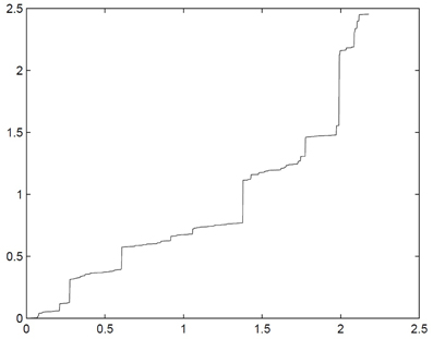
Figure 1. Simulated sample path of the tempered stable subordinator T with parameters α = 1.2 and θ = 0.8.

FIGURE 2

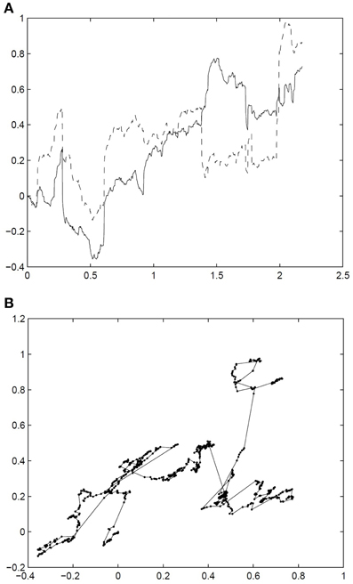
Figure 2. Simulated sample path of the 2 dimensional standard fractional NTS process X = (X₁(t), X₂(t))_{t ≥ 0} with parameters α = 1.2, θ = 0.8, β = (0.1, −0.3), σ_{1, 2} = σ_{2, 1} = 0.7, and H = 0.6525.

5. ARMA-GARCH Model with fNTS Innovations and Empirical Illustration

Let X ~ fstdNTS_N (H, α, θ, β, Σ) generated by Z ~ stdNTS_N (α, θ, β, Σ). A N-dimensional discrete time process Y = (Y(k))_{k ∈ {0, 1, 2, … }} with Y(k) =(Y₁(k), Y₂(k), …, Y_N(k)) is referred to as the N-dimensional ARMA-GARCH model with fNTS innovations when it is given by the ARMA(1,1) - GARCH(1,1) model as follows: Y_n(0) = 0, ε_n(0) = 0, and

$\begin{array}{cc}\{\begin{array}{l}\begin{array}{ll}{Y}_n(k+1)\hfill & \text{}\text{}\text{}=c_n+a_n{Y}_n(k)+b_n{\sigma }_n(k){\epsilon }_n(k)\hfill \\ \hfill & +{\sigma }_n(k+1){\epsilon }_n(k+1)\hfill \end{array}\hfill \\ {({\sigma }_n(k+1))}^2={\kappa }_n+{\xi }_n{({\sigma }_n(k){\epsilon }_n(k))}^2+{\zeta }_n{({\sigma }_n(k))}^2\hfill \end{array}\text{}\text{}\text{}\text{}\text{},& (13)\end{array}$

where ε_n(k + 1) = X_n(k + 1) − X_n(k) and n ∈ {1, 2, …, N}. This model describes volatility clustering effect by GARCH(1,1) model, the fat-tails and the asymmetric dependence between elements by the standard NTS process Z, and the long-range dependence by fractional NTS process X.

Since we have

$X_n(k)\approx {\displaystyle \sum _{j=0}^{k-1}{K}_H}(k,j)(Z_n(j+1)-Z_n(j))$

The increment X_n(k + 1)−X_n(k) can be approximated as follows:

$\begin{array}{cc}\begin{array}{l}{X}_n(k+1)-X_n(k)\\ \approx K_H(k+1,k)(Z_n(k+1)-Z_n(k))\\ +{\displaystyle \sum _{j=0}^{k-1}(K_H(}k+1,j)-K_H(k,j))(Z_n(j+1)-Z_n(j))\end{array}& (14)\end{array}$

Let M be the number of time steps in the sample and N be the number of assets in the portfolio. ARMA(1,1)-GARCH(1,1) model is fit to the data and extract ε_n(t_k), for n = 1, 2, …, N and k = 1, …, M. Since Equation (8) is the same as the covariance of the fractional Brownian motion, set $W_n(t_k)={\displaystyle {\sum }_{j=1}^k{\epsilon }_n}(t_j)$ and estimate the Hurst index H_n of the process (W_n(t_k))_{tk ≥ 0} using the wavelet details regression estimator method by Flandrin [23] and Abry et al. [24]. The parameter H is obtained finally as the mean of H_n for n = 1, 2, …, N.

Suppose we have estimated Hurst index H. We estimate the parameters of the model as follows in this investigation.

1. Estimate ARMA(1,1)-GARCH(1,1) parameters a_n, b_n, c_n, κ_n, ξ_n, and ζ_n with standard normal innovations by maximum likelihood estimation (MLE) with assumption (σ_n(0))² = κ_n/(1 − ξ_n − ζ_n) for n = 1, 2, …, N.

2. Extract residuals using the estimated parameters.

3. Put $X_n(t_k)={\displaystyle {\sum }_{j=1}^k{\epsilon }_n}(t_j)$ and extract {Z_n(t_k)| k = 1, 2, …, M} for n = 1, 2, …, N as follows.

$\begin{array}{cc}\begin{array}{l}{Z}_n(1)=X_n(1)/K_H(1,0)\text{ and}\\ Z_n(k)=Z_n(k-1)+\frac{X_n(k)-X_n(k-1)}{K_H(k,k-1)}\\ -{\displaystyle \sum _{j=0}^{k-2}\frac{K_H(k,j)-K_H(k-1,j)}{K_H(k,k-1)}}(Z_n(j+1)-Z_n(j))\end{array}& (15)\end{array}$

for k = 2, 3, …, M.

4. Estimate parameters α_n, θ_n, and β_n of the standard NTS process using {Z_n(k)| k = 1, 2, …, M} extracted in the step 4 by curve-fitting in least-squares sense. Set $\alpha ={\displaystyle {\sum }_{n=1}^N\frac{{\alpha }_n}{N}}$ and $\theta ={\displaystyle {\sum }_{n=1}^N\frac{{\theta }_n}{N}}$ Estimate parameters β_n again using {Z_n(k)| k = 1, 2, …, M} by means of MLE for n = 1, 2, …, N.

5. Calculate the covariance between (Z_m(1)) and (Z_n(1)) for m,n ∈ {1, 2, …, N} using data {(Z_m(k), Z_n(k))| k =1, 2, …, M} extracted in the step 4. Estimate

$\Sigma ={[{\sigma }_{m,n}]}_{m,n\in \{1,2,\cdots ,N\}}$

by Equation (4) and cov(Z_m(1), Z_n(1)).

The parameter H is estimated using 2,158 observed 1 min returns for five stocks (Apple Inc., Google Inc., IBM Co., A&T, Wal-Mart Stores Inc.) from November 21 to November 29, 2011. Set dt = 1/390, since 1 day has 6 h and 30 min (from 9:30 to 16:00) trading time, that is 390 min, on New York Stock Exchange. The parameters H_n are presented in Table 1 and parameter H = 0.5806 is obtained finally as the mean of H_n.

TABLE 1

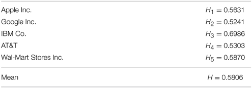
Table 1. Estimated Hurst index H_n.

The ARMA(1,1)-GARCH(1,1) parameters and estimated fNTS parameters α, θ and β are reported in Table 2 for each stocks. The estimated matrix Σ is presented in Table 3.

TABLE 2

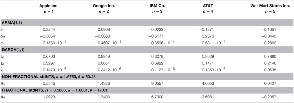
Table 2. Parameters the ARMA-GARCH model with (non-fractional) NTS innovations and fNTS innovations.

TABLE 3

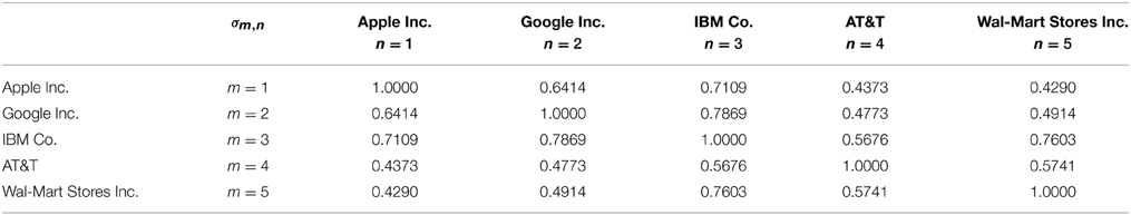
Table 3. Estimated Σ = [σ_m,n]_{m,n ∈ {1, 2, …, N}}.

The Kolmogorov-Smirnov (KS) and Anderson-Darling (AD) tests are used for goodness-of-fit tests. The KS and AD² statistic are given by

$KS={\displaystyle \sum _x|}\widehat{F}(x)-F(x)|, A{D}^2=s{\displaystyle {\int }_{-\infty }^{\infty }\frac{{(\widehat{F}(x)-F(x))}^2}{F(x)(1-F(x))}}dF(x),$

where $\widehat{F}(x)$ is the empirical sample distribution, F(x) is the estimated theoretical distribution, and s is the number of observed samples. According to the p-values of KS statistic and AD² statistic, estimated parameters are not rejected. Calculating p-values for KS and AD² statistic are explained in Marsaglia et al. [25] and Marsaglia and Marsaglia [26]. The KS and AD² statistics are calculated between the standard NTS distribution with estimated parameters (α, θ, β_n), and the empirical cumulative distribution of {Z_n(t_k) − Z_n(t_{k − 1})| k = 1, 2, …, M} where Z_n(t_k) is the extracted process by Equation (15). According to the p-values of KS and AD² statistic in Table 4, all estimated parameters are not rejected at the 1% significance level for the five stock returns investigated.

TABLE 4

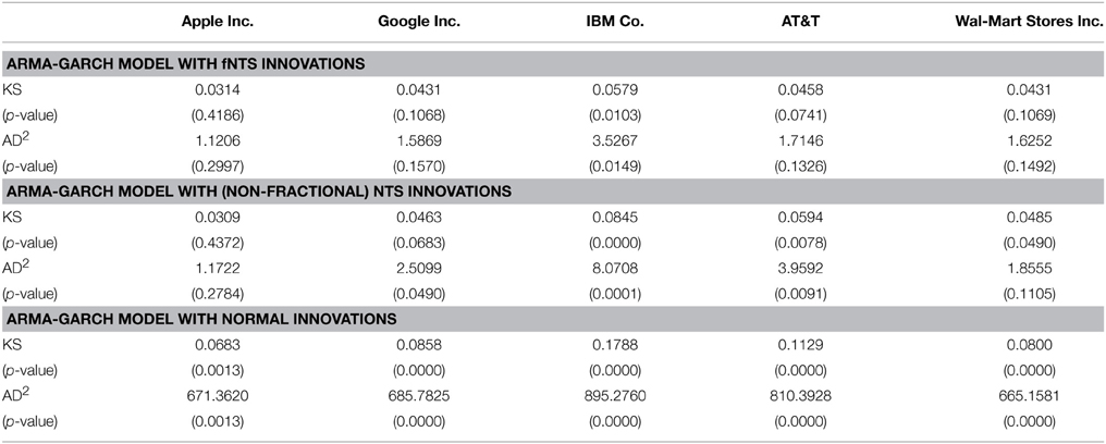
Table 4. Goodness-of-fit test for the ARMA-GARCH model with normal innovations.

If H = 0.5 then the ARMA-GARCH model with fNTS innovations becomes the ARMA-GARCH model with non-fractional NTS innovations. The estimated parameters of the non-fractional standard NTS process are presented also in Table 2 for each stocks. To compare the performance of parameter estimation for ARMA-GARCH model with fNTS innovations with non-fractional NTS innovation, we provide KS and AD² statistic with p-values for the ARMA-GARCH model with non-fractional NTS innovations in Table 4 as well. Unfortunately, the estimated parameters for IBM Co. and AT&T are rejected by KS and AD tests at the 1% significance level.

If we assume that (ε_n(t_k))_{k = 1, 2, …, M} is independent and identically distributed and ε_n(t_k) ~ N(0, 1), then the Y_n follows the ARMA-GARCH model with normal innovations. The ARMA-GARCH model with normal innovations is rejected by both KS test and and AD test for all considered stocks at the 1% significance level.

Therefore, we can conclude that the ARMA-GARCH model with fNTS innovations describes behavior of the high frequency return time series investigated in this section. While, the ARMA-GARCH models with non-fractional NTS innovations and normal innovations do not perfectly explain the behavior of the high frequency return data.

6. Assessment Risk on the ARMA-GARCH Model with fNTS Innovations

In this section, portfolio VaR and AVaR on the ARMA-GARCH model with fNTS innovations are discussed, and they are applied to the portfolio optimization.

Let > 0 be a time horizon. Assume that we have a portfolio with N stocks. Suppose the stock return vector process Y = (Y(t_k))_{k ∈ {0, 1, 2, …, M}} with Y(t_k) = (Y₁(t_k), Y₂(t_k), …, Y_N(t_k)) follows the ARMA-GARCH model with fNTS innovations as defined in Section 5 and X ~ fstdNTS_N (H, α, θ, β, Σ) generated by Z~ stdNTS_N (α, θ, β, Σ), where {t₀, t₁,…, t_M} is a given discrete time such that t_k = k · Δt with Δt =/M for k ∈ {0, 1, 2, …, M}. Then a portfolio return process R = (R(t_k))_{k ∈ {0, 1, 2, …, M}} with allocation weight vector w = (w₁, w₂, …, w_N)^T with ${\displaystyle {\sum }_{n=1}^N{w}_n}=1$ is given by $R(t_k)={\displaystyle {\sum }_{n=1}^N{w}_n}{Y}_n(t_k)$.

We have

$\begin{array}{cc}\begin{array}{l}R(k+1)={\displaystyle \sum _{n=1}^N{w}_n}{Y}_n(k+1)\\ ={\displaystyle \sum _{n=1}^N{w}_n}(c_n+a_n{Y}_n(k)+b_n{\sigma }_n(k){\epsilon }_n(k))\\ +{\displaystyle \sum _{n=1}^N{w}_n}{\sigma }_n(k+1){\epsilon }_n(k+1)\end{array}& (16)\end{array}$

and

$\begin{array}{l}{\displaystyle \sum _{n=1}^N{w}_n}{\sigma }_n(k+1){\epsilon }_n(k+1)\\ ={\displaystyle \sum _{n=1}^N{w}_n}{\sigma }_n(k+1)\frac{X_n(k+1)-X_n(k)}{{(t_{k+1}-t_k)}^H}\\ ={(\Delta t)}^{-H}{\displaystyle \sum _{n=1}^N{w}_n}{\sigma }_n(k+1)(X_n(k+1)-X_n(k)).\end{array}$

By Equation (14), we obtain

$\begin{array}{cc}\begin{array}{l}{\displaystyle \sum _{n=1}^N{w}_n}{\sigma }_n(k+1){\epsilon }_n(k+1)\\ \approx {(\Delta t)}^{-H}{K}_H(t_{k+1},t_k){\displaystyle \sum _{n=1}^N{w}_n}{\sigma }_n(k+1)(Z_n(k+1)-Z_n(k))\\ +{(\Delta t)}^{-H}{\displaystyle \sum _{n=1}^N{\displaystyle \sum _{j=0}^{k-1}{w}_n}}{\sigma }_n(k+1)(K_H(t_{k+1},t_j)\\ -K_H(t_k,t_j))(Z_n(t_{j+1})-Z_n(t_j))\end{array}& (17)\end{array}$

Let ((t_k))_{k ∈ {1, 2, …, M}} be the natural filtration generated by Y. Then σ_n(k + 1) and

$\begin{array}{l}{\displaystyle \sum _{n=1}^N{\displaystyle \sum _{j=0}^{k-1}{w}_n}}{\sigma }_n(k+1)(K_H(t_{k+1},t_j)\\ -K_H(t_k,t_j))(Z_n(t_{j+1})-Z_n(t_j))\end{array}$

are (t_k)-measurable. Moreover, since Z_n has stationary increments, we have

Hence, we have

where (Ξ(t))_{t ≥ 0} ~ NTS₁(α, θ, β, γ, 1) with

$\begin{array}{l}\overline{\beta }={\displaystyle \sum _{n=1}^N{w}_n}{\sigma }_n(k+1){\beta }_n,\\ \overline{\gamma }=\sqrt{{\displaystyle \sum _{m=1}^N{\displaystyle \sum _{n=1}^N{w}_m}}{w}_n{\sigma }_m(k+1){\sigma }_n(k+1){\sigma }_{m,n}{\gamma }_m{\gamma }_n},\end{array}$

and

${\gamma }_n=\sqrt{1-{\beta }_n^2\left(\frac{1-\alpha }{2\theta }\right)}, n=1,2,\cdots ,N,$

by Proposition 1. Therefore, we can discuss VaR and AVaR as follows. The VaR and AVaR for R(k + 1) with the significance level η under information until time t_k are defined by

and

respectively. By Equation (16), we have

and by Equation (17), we obtain

Thus, by Equation (18) we obtain

By the same argument, we obtain AVaR as follows

The closed-form solutions of VaR_η (Ξ(Δt)) and AVaR_η (Ξ(Δt)) for NTS process (Ξ(t))_{t ≥ 0} is presented in Kim et al. [27].

The Figures 3A,B exhibit the forecasted 1 min ahead VaR and AVaR values, respectively, for an equally weighted portfolio for the five stocks in this study based on the parameters in Table 2 and information we discussed in the Section 5. The equally weighted portfolio is the portfolio having allocation weight as w = (1/N, 1/N, …, 1/N), where N is the number of stocks in the portfolio. The forecasted 1-min VaR and AVaR values are calculated by Equation (19) and Equation (20), respectively, at confidence levels from 0.5 to 10%. The VaR and AVaR values for the portfolio based on the ARMA-GARCH model with non-fractional NTS innovations are presented in the figure. The VaR (AVaR) values of the ARMA-GARCH model with fNTS innovations are larger than VaR (AVaR) values of the model with non-fractional NTS innovations.

FIGURE 3

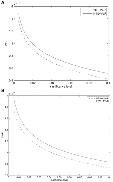
Figure 3. Forecasted 1 min (A) VaR and (B) AVaR under the ARMA-GARCH model with non-fractional NTS and fNTS innovations. VaR and AVaR values for the ARMA-GARCH model with fNTS innovations are given by solid curves, and those values for the ARMA-GARCH model with non-fractional NTS innovations are given by dash curves.

7. Portfolio Optimization and Risk Budgeting on the ARMA-GARCH Model with fNTS Innovations

Using VaR and AVaR values by Equation (19) and Equation (20), we can find the optimal portfolio. The VaR minimizing portfolio is obtained by solving the following optimization problem:

where μ₀ is the benchmark expected return. Similarly, the AVaR minimizing portfolio is obtained by solving the following optimization problem:

Table 5 presents the VaR and AVaR minimizing portfolios with the benchmark return μ₀ = 2.5924 · 10⁻⁴. To measure performance of the optimal portfolio, we use the VaR ratio and stable tail-adjusted return ratio (STARR), which are defined by

and

respectively⁵. The following is concluded from the results reported in Table 5:

• The VaR minimizing portfolio has the best expected return among the three portfolios.

• The AVaR minimizing portfolio has smaller VaR than the case of the VaR minimizing portfolio, but that is not surprising since the AVaR minimizing portfolio has less expected return than the case of the VaR minimizing portfolio.

• The AVaR minimizing portfolio has the largest VaR Ratio among the three VaR ratios.

• The AVaR minimizing portfolio has the largest STARR among the three STARR.

TABLE 5

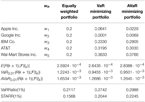
Table 5. Optimal allocation weight for the portfolio with the five stocks and performance measures.

8. Conclusion

The multivariate ARMA-GARCH model with fNTS innovations exhibits fat-tails, asymmetric dependence, volatility clustering, and long-range dependence. Comparing with two ARMA-GARCH models with non-fractional NTS innovation and normal innovations, the ARMA-GARCH model with fNTS innovations has better performance in parameter estimation for 1-min stock return data investigated in this paper. That means the fNTS process describes the behavior of the residual process of 1-min returns better than the non-fractional NTS process or Brownian motion. The portfolio VaR and AVaR are calculated by the approximation method under the model, and those risk measures are used for portfolio optimization. In this investigation, we obtain the fact that the risk measures of the ARMA-GARCH model with fNTS innovations are more conservative than those of the model with non-fractional NTS innovations. The AVaR minimizing portfolio performs better than the VaR minimizing portfolio for the case considered in this paper.

Conflict of Interest Statement

The author declares that the research was conducted in the absence of any commercial or financial relationships that could be construed as a potential conflict of interest.

Footnotes

1. ^Kim [15] defines another different multivariate fractional NTS process using the time-changed fractional Brownian motion.

2. ^AVaR is also known as conditional value-at-risk (CVaR). See Pflug [16] and Rockafellar and Uryasev [17, 18].

3. ^VaR is not is not a coherent risk measure. The notion of a coherent risk measure was introduced by Artzner et al. [19].

4. ^The tempered stable subordinator T with parameter (α, θ) is included in the class of tempered stable processes provided by Rosinski [8]. The parameter α/2 of the tempered stable subordinator corresponds to the parameter α in Rosinski's tempered stable class.

5. ^Many literatures define the VaR ratio and STARR as

and

respectively, where R_f is a market index return. In this paper, we assume R_f = 0 for considering absolute performance.

References

Mandelbrot BB, Ness JWV. Fractional brownian motions, fractional noises applications. SIAM Rev. (1968) 10, 422–37. doi: 10.1137/1010093

CrossRef Full Text | Google Scholar

Engle R. Autoregressive conditional heteroskedasticity with estimates of the variance of United Kingdom inflation. Econometrica (1982) 50, 987–1007. doi: 10.2307/1912773

CrossRef Full Text | Google Scholar

Bollerslev T. Generalized autoregressive conditional heteroskedasticity. J Econometr. (1986) 31:307–27. doi: 10.1016/0304-4076(86)90063-1

CrossRef Full Text | Google Scholar

Sun W, Rachev ST, Fabozzi FJ. Long-range dependence, fractal processes, and intra-daily data. In: Seese D, Weinhardt C, Schlottmann F. editors. Handbook on Information Technology in Finance (2008). (Springer), p. 543–85.

Beck A, Kim YS, Rachev ST, Feindt M, Fabozzi FJ. Empirical analysis of ARMA-GARCH models in market risk estimation on high-frequency U.S. data. Stud Nonlin Dyn Econometri. (2012). 17:167–77. doi: 10.1515/snde-2012-0033

CrossRef Full Text | Google Scholar

Sun W, Rachev ST, Fabozzi FJ. Fractals or I.I.D.: evidence of long-range dependence and heavy tailedness from modeling German equity market returns. J Econ Bus. (2007) 59:575–95. doi: 10.1016/j.jeconbus.2007.02.001

CrossRef Full Text | Google Scholar

Houdre C, Kawai R. On fractional tempered stable motion. Stochast Process Appl. (2006) 116:1161–84. doi: 10.1016/j.spa.2006.01.008

CrossRef Full Text | Google Scholar

Rosiński J. Tempering stable processes. Stochast Proce Appl. (2007) 117:677–707. doi: 10.1016/j.spa.2006.10.003

CrossRef Full Text

Barndorff-Nielsen OE, Shephard N. Normal Modified Stable Processes. Economics Series Working Papers from University of Oxford, Department of Economics. (2001) 72.

Google Scholar

Barndorff-Nielsen OE, Levendorskii S. Feller processes of normal inverse gaussian type. Quantitat Finan. (2001) 1:318–31. doi: 10.1088/1469-7688/1/3/303

CrossRef Full Text | Google Scholar

Eberlein E, Madan DB. On correlating lévy processes. J Risk. (2010) 13:3–16.

Kim YS, Giacometti R, Rachev ST, Fabozzi FJ, Mignacca D. Measuring financial risk and portfolio optimization with a non-Gaussian multivariate model. Anna Operat Res. (2012) 201:325–43. doi: 10.1007/s10479-012-1229-8

CrossRef Full Text | Google Scholar

Kim YS, Volkmann D. Normal tempered stable copula. Appl Math Lett. (2013). 26:676–80. doi: 10.1016/j.aml.2013.01.009

CrossRef Full Text | Google Scholar

Kim YS, Rachev ST, Chung DM, Bianchi ML. The modified tempered stable distribution, GARCH-models and option pricing. Probabil Math Stat. (2009) 29:91–117.

Google Scholar

Kim YS. Fractional multivariate normal tempered stable process. Appl Math Lett. (2012) 25:2396–401. doi: 10.1016/j.aml.2012.07.011

CrossRef Full Text | Google Scholar

Pflug G. Some Remarks on the value-at-risk and the Conditional value-at-risk. In: Uryasev S, editor. Probabilistic Constrained Optimization: Methodology and Applications. Kluwer Academic Publishers (2000). p. 272–281.

Rockafellar RT, Uryasev S. Optimization of conditional value-at-risk. J Risk (2000) 2:21–41.

Google Scholar

Rockafellar RT, Uryasev S. Conditional value-at-risk for general loss distributions. J Bank Finance. (2002) 26:1443–71. doi: 10.1016/S0378-4266(02)00271-6

CrossRef Full Text | Google Scholar

Artzner P, Delbaen F, Eber JM, Heath D. Coherent measures of risk. Math Finance. (1999) 9:203–28. doi: 10.1111/1467-9965.00068

CrossRef Full Text | Google Scholar

Rachev ST, Stoyanov S, Fabozzi FJ. Advanced Stochastic Models, Risk Assessment, and Portfolio Optimization: The Ideal Risk, Uncertainty, and Performance Measures. Hoboken, NJ: John Wiley & Sons (2007).

Markowitz HM. Portfolio selection. J Finance. (1952) 7:77–91.

Google Scholar

Samorodnitsky G, Taqqu MS. Stable Non-Gaussian Random Processes. Chapman & Hall/CRC (1994). (Baca Raton, London, New York, Washinton, DC).

Google Scholar

Flandrin P. Wavelet analysis and synthesis of fractional Brownian motion. IEEE Trans Inf Theory. (1992) 38:910–17. doi: 10.1109/18.119751

CrossRef Full Text | Google Scholar

Abry P, Flandrin P, Taqqu MS, Veitch D. Self-similarity and long-range dependence through the wavelet lens. In: Theory and Applications of Long-Range Dependence. Birkhäuser (2003). eds D. Paul, O. George and T. Murad p. 527–556.

Marsaglia G, Tsang WW, Wang G. Evaluating kolmogorov's distribution. J Stat Softw. (2003) 8:1–4.

Marsaglia G, Marsaglia J. Evaluating the anderson-darling distribution. J Stat Softw. (2004) 9:1–5.

Google Scholar

Kim YS, Rachev ST, Bianchi ML, Fabozzi FJ. Computing VaR and AVaR in infinitely divisible distributions. Probab Math Stat. (2010) 30:223–45.

Google Scholar

Nualart D. Stochastic integration with respect to fractional Brownian motion and applications. Contemp Math. (2003) 336:3–39. doi: 10.1090/conm/336/06025

CrossRef Full Text | Google Scholar

Appendix

To define a process with long-range dependence, we use the Volterra kernel K_H:[0, ∞) × [0, ∞) → [0, ∞), given by

$c_H={\left(\frac{H(1-2H)\Gamma (\frac{1}{2}-H)}{\Gamma (2-2H)\Gamma (H+\frac{1}{2})}\right)}^{\frac{1}{2}}.$

with

${\displaystyle {\int }_0^{t\wedge s}{K}_H}(t,u)K_H(s,u)du=\frac{1}{2}\left(t^{2H}+s^{2H}-|t-s{|}^{2H}\right),$

and H ∈ (0, 1). According to Nualart [28] and Houdre and Kawai [7], we have the following facts:

• We have

${\displaystyle {\int }_0^t{K}_H}{(t,s)}^{2}ds=t^{2(H-\frac{1}{2})+1}.$

and

$\begin{array}{cc}{\displaystyle {\int }_0^t{K}_H}{(t,s)}^{2}ds=t^{2(H-\frac{1}{2})+1}.& (22)\end{array}$

• If H ∈ (½, 1) then

$\begin{array}{l}{K}_H(t,s)=c_H\left(H-\frac{1}{2}\right)s^{\frac{1}{2}-H}\\ {\displaystyle {\int }_s^t{(u-s)}^{H-\frac{3}{2}}}{u}^{H-\frac{1}{2}}du{1}_{[0,t]}(s).\end{array}$

Moreover, K_½(t, s) = 1_{[0, t]}(s).

• Let t > 0 and let p ≥ 2. K_H(t, ·) ∈ L^p([0, t]) if and only if !!i!!. When K_H(t, ·) ∈ L^p([0, t]), we have

${\displaystyle {\int }_0^t{K}_H}{(t,s)}^{p}ds=C_{H,p}{t}^{p(H-\frac{1}{2})+1},$

where

$\begin{array}{cc}\begin{array}{l}{C}_{H,p}=c_H^p{\displaystyle {\int }_0^1{v}^{p\left(\frac{1}{2}-H\right)}}\times [{(1-v)}^{H-\frac{1}{2}}-\left(H-\frac{1}{2}\right)\\ {{\displaystyle {\int }_v^1{w}^{H-\frac{3}{2}}}{(w-v)}^{H-\frac{1}{2}}dw]}^{p}dv.\end{array}& (23)\end{array}$