Efficient Spectral Estimation by MUSIC and ESPRIT with Application to Sparse FFT

1. Introduction

The problem of spectral estimation resp. frequency analysis arises quite often in signal processing, electrical engineering, and mathematical physics (see e.g., the books [1, 2] or the survey [3]) and reads as follows:

(P1) Recover the positive integer M, the distinct frequencies ${\phi }_j\in (-\frac{1}{2},\frac{1}{2}]$, and the complex coefficients c_j ≠ 0 (j = 1, …, M) in the exponential sum of sparsity M

$\begin{array}{ll}h(x):\text{}={\displaystyle \sum _{j=1}^M}{c}_j{\text{e}}^{2\pi \text{i}{\phi }_{j}x}(x\in ℝ),\hfill & (1.1)\hfill \end{array}$

if noisy sampled data ${\tilde{h}}_k:=h(k)+e_k$ (k = 0, …, N − 1) with N ≥ 2M are given, where e_k ∈ ℂ are small error terms with $|e_k|\le \frac{1}{10}\underset{j}{min}|c_j|$.

Introducing so-called left/right signal spaces and noise spaces in Section 2, we explain the numerical solution of the problem (P1) by the MUSIC method (created by Schmidt [4], see also Manolakis et al. [1, Section 9.6.3] and the references therein) and the ESPRIT method (created by Roy and Kailath [5], see also Manolakis et al. [1, Section 9.6.5], Stoica and Moses [2, Chapter 4] and the references therein). In a new unified approach to MUSIC and ESPRIT, we show that both methods are based on singular value decomposition (SVD) of a rectangular Hankel matrix of given sampled data. For the MUSIC and ESPRIT method, it is important to choose the window length L (number of rows) of the rectangular Hankel matrix in an optimal way. Based on Theorem 2.5, where we estimate the singular values and the spectral norm condition number of the rectangular Hankel matrix of noiseless data, one can see that $L\approx \frac{N}{2}$ is a good choice. By the right choice of L, one can detect the correct sparsity M of (1.1) and avoid the computation of spurious frequencies.

The main disadvantages of MUSIC and ESPRIT are the relatively high computational cost in the case of large sparsity M, caused mainly by the SVD. The known algorithms for MUSIC and ESPRIT have moderate computational cost only for small sparsity M. Thus, following question arises: How can one improve the MUSIC and ESPRIT methods for spectral estimation of exponential sums with large sparsity M? In this paper, we show that this is possible by a special divide-and-conquer technique. In the numerical examples of Section 5, the cases M = 256 and M = 1024 are handled.

The computational cost of an algorithm is measured in the number of arithmetical operations, where all operations are counted equally. Often the computational cost of an algorithm is reduced to the leading term, i.e., all lower order terms are omitted. For a unified approach to Prony–like methods for the parameter estimation of (1.1), namely the classical Prony method, the matrix pencil method [6, 7], and the ESPRIT method [5, 8], we refer also to Potts and Tasche [9] and the references therein. For a survey of the most successful methods for the data fitting problem with linear combinations of complex exponentials, we refer to Pereyra and Scherer [10].

Section 3 is the core of this paper. Here we present a new efficient spectral estimation with low computational cost for large sparsity M and a moderate number of given samples, if one has to recover a trigonometric polynomial of large sparsity M. This means we specialize the problem (P1). Let S > 0 be a large even integer. Assume that ${\phi }_j=\frac{{\omega }_j}{S}\in (-\frac{1}{2},\frac{1}{2}]$, where ${\omega }_j\in (-\frac{S}{2},\frac{S}{2}]\cap \mathbb{Z}$. Replacing the variable x by Sx in (1.1), we consider the 1-periodic trigonometric polynomial of sparsity M

$\begin{array}{ll}g(x):\text{}=h(Sx):\text{}={\displaystyle \sum _{j=1}^M}{c}_j{\text{e}}^{2\pi \text{i}{\omega }_{j}x}(x\in ℝ)\hfill & (1.2)\hfill \end{array}$

with integer frequencies ${\omega }_j\in (-\frac{S}{2},\frac{S}{2}]\cap \mathbb{Z}$. Consequently we investigate the following spectral estimation problem:

(P2) Recover the sparsity M ∈ ℕ, all integer frequencies ${\omega }_j\in (-\frac{S}{2},\frac{S}{2}]\cap \mathbb{Z}$ as well as all non-zero coefficients c_j ∈ ℂ of the trigonometric polynomial (1.2) for noisy sampled values ${\tilde{g}}_k:=g(\frac{k}{S})+e_k=h(k)+e_k$ (k = 0, …, N − 1) with N ≥ 2M, where e_k ∈ ℂ are small error terms with $|e_k|\le \frac{1}{10}\underset{j}{min}|c_j|$. Often one considers the modified problem (P2*), where the sparsity M is known.

A numerical solution of problem (P2) or (P2*) with low computational cost is called sparse fast Fourier transform (sparse FFT). Using divide-and-conquer technique, the trigonometric polynomial (1.2) of large sparsity M is split into some trigonometric polynomials of lower sparsity and corresponding samples are determined by fast Fourier transform (FFT). Here we borrow an idea from sparse FFT in Lawlor et al. [11] and Christlieb et al. [12] and use shifted sampling of (1.2), i.e., equidistant sampling with few equidistant shifts. Then the trigonometric polynomials of lower sparsity can be recovered by MUSIC resp. ESPRIT. The computational cost of the new sparse FFT is analyzed too.

A similar splitting technique is suggested in Lawlor et al. [11] and Christlieb et al. [12], but with a different method to detect frequencies, when aliasing between two or more frequencies occurs. The method in Lawlor et al. [11] and Christlieb et al. [12] follows an idea of Iwen [13], which is based on the Chinese Remainder Theorem, see also Ben-Or and Tiwari [14]. A different method for the sparse FFT, based on efficient filters is suggested in Hassanieh et al. [15] and Gilbert et al. [16]. We remark that there are two types of methods, deterministic (see [13]) and randomized (see [15, 11, 16]). Further related randomized methods based on compressed sensing can be found in the papers [17, 18, 19] and in the monograph [20]. Please note that the sparse FFT methods mentioned before solve the problem (P2*), i.e., one assumes that the sparsity (or an upper bound) is known, whereas our new deterministic sparse FFT also detects the sparsity M. We remark that preliminary tests of the implementation [21, 22] of the sfft version 3 algorithm [15] suggest that this method also works if the sparsity input parameter is chosen larger than the actual sparsity of the signal. For further references on sparse FFTs, we refer to Remark 3.1.

In Section 4, we extend our method to a new reconstruction of multivariate trigonometric polynomials of large sparsity, where sampled data on a convenient rank-1 lattice are given. In Section 5, several numerical experiments with noiseless resp. noisy sampled data illustrate the high performance of the sparse FFT as proposed in Section 3. Note that in the case of successful recovery of the sparse trigonometric polynomial (1.2) all frequencies are correctly detected. For the modified sparse FFT of Section 4, numerical examples for the reconstruction of six-variate trigonometric polynomials of sparsity 256 are given too. Moreover, we compare our results with preliminary tests of the implementation [21, 22] of the sfft version 3 algorithm [15].

In summary we present a splitting method, in between the well-known methods ESPRIT, MUSIC, and FFT for the problem (P2) with the parameters in Table 1. For the results, see the Tables 3, 4 in Section 3. Furthermore, we use a reconstructing rank-1 lattice in order to reconstruct multivariate trigonometric polynomials, see Section 4. Here in the case of successful recovery of a sparse multivariate trigonometric polynomial, all frequency vectors are detected without errors.

TABLE 1

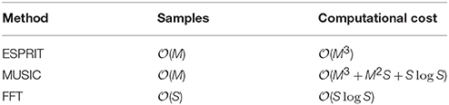
Table 1. Numbers of required samples and computational costs for ESPRIT, MUSIC, and FFT, where M denotes the sparsity of (1.1) and S is a large even integer so that all frequencies φ_j are of the form $\frac{{\omega }_j}{S}$ with ${\omega }_j\in (-\frac{S}{2},\frac{S}{2}]\cap \mathbb{Z}$.

2. Reconstruction of Exponential Sums

The main difficulty is the recovery of the frequency set Φ: = {φ₁, …, φ_M} in (1.1).

We introduce the rectangular Fourier–type matrix ${\mathit{\text{F}}}_{N,M} :={\left(e^{2\pi i{\phi }_j(k-1)}\right)}_{k,j=1}^{N,M}.$ Note that F_{N, M} coincides with the rectangular Vandermonde matrix ${\mathbf{V}}_{N,M}(\mathbf{z}):={(z_j^{k-1})}_{k,j=1}^{N,M}$ with $\mathbf{z}:={(z_j)}_{j=1}^M$, where $z_j:={\text{e}}^{2\pi \text{i}{\phi }_j}$ (j = 1, …, M) are distinct nodes on the unit circle. Then the spectral estimation problem can be formulated in following matrix-vector form

$\begin{array}{ll}{V}_{N,M}(z)c=\tilde{h},\hfill & (2.1)\hfill \end{array}$

where $\tilde{\mathbf{h}}:={({\tilde{h}}_k)}_{k=0}^{N-1}$ is the vector of noisy sampled data and $\mathbf{c}:={(c_j)}_{j=1}^M$ the vector of complex coefficients of (1.1).

Under the natural assumption that the nodes z_j (j = 1, …, M) are well-separated on the unit circle, it can be shown that F_{P, M} has a uniformly bounded spectral norm condition number for sufficiently large integer P > M.

Theorem 2.1 (see [23, Theorem 2]) Assume that the frequencies ${\phi }_j\in (-\frac{1}{2},\frac{1}{2}]$ (j = 1, …, M) are well-separated by the separation distance

$q:\text{}=\underset{j\ne \ell }{\min }(\underset{n\in \mathbb{Z}}{\min }|{\phi }_j+n-{\phi }_{\ell }|)>0$

and that $P>max\left\{M,2\pi +\frac{1}{q}\right\}$.

Then the discrete Ingham inequalities related to F_{P, M} indicate that for all x ∈ ℂ^M

$\begin{array}{ll}{\alpha }_1(P)\Vert x{\Vert }_2^2\le \Vert F_{P,M}x{\Vert }_2^2\le {\alpha }_2(P)\Vert x{\Vert }_2^2\hfill & (2.2)\hfill \end{array}$

with ${\alpha }_1(P) :=P\left(\frac{2}{\pi }-\frac{2}{\pi P^2{q}^2}-\frac{4}{P}\right)$ and

${\alpha }_2(P):\text{}=\{\begin{array}{ll}P(\frac{4\sqrt{2}}{\pi }+\frac{\sqrt{2}}{\pi P^2{q}^2}+\frac{3\sqrt{2}}{P})\hfill & forevenP,\hfill \\ (P+1)(\frac{4\sqrt{2}}{\pi }+\frac{\sqrt{2}}{\pi {(P+1)}^2{q}^2}+\frac{3\sqrt{2}}{P+1})\hfill & foroddP.\hfill \end{array}$

Furthermore, the rectangular Fourier–type matrix F_{P, M} has a uniformly bounded spectral norm condition number

${\text{cond}}_2{F}_{P,M}\le \sqrt{\frac{{\alpha }_2(P)}{{\alpha }_1(P)}}.$

Proof. The assumption $P>2\pi +\frac{1}{q}$ is sufficient for the gap condition

$\begin{array}{ll}q>\frac{1}{P}{\left(1-\frac{2\pi }{P}\right)}^{-1/2}\hfill & (2.3)\hfill \end{array}$

to hold. The gap condition (2.3) ensures that α₁(P) > 0. For a proof of the discrete Ingham inequalities (2.2) under the gap condition (2.3) see Liao and Fannjiang [23, Theorem 2]. Let λ₁ ≥ … ≥ λ_M > 0 be the ordered eigenvalues of ${\mathbf{F}}_{P,M}^{*}{\mathbf{F}}_{P,M}\in {\mathbf{C}}^{M\times M}$. Using the Raleigh–Ritz Theorem and (2.2), we obtain that for all x ∈ ℂ^M

${\alpha }_1(P)\Vert x{\Vert }_2^2\le {\lambda }_M\Vert x{\Vert }_2^2\le \Vert F_{P,M}x{\Vert }_2^2\le {\lambda }_1\Vert x{\Vert }_2^2\le {\alpha }_2(P)\Vert x{\Vert }_2^2$

and hence

$\begin{array}{ll}0<{\alpha }_1(P)\le {\lambda }_M\le {\lambda }_1\le {\alpha }_2(P)<\infty .\hfill & (2.4)\hfill \end{array}$

Thus, ${\mathbf{F}}_{P,M}^{*}{\mathbf{F}}_{P,M}$ is positive definite and

${\text{cond}}_2{F}_{P,M}=\sqrt{\frac{{\lambda }_1}{{\lambda }_M}}\le \sqrt{\frac{{\alpha }_2(P)}{{\alpha }_1(P)}}.$

This completes the proof. □

Corollary 2.2 Assume that the frequencies ${\phi }_j\in (-\frac{1}{2},\frac{1}{2}]$ (j = 1, …, M) are well-separated by the separation distance q > 0 and that $P>max\left\{M,2\pi +\frac{1}{q}\right\}$.

Then the discrete Ingham inequalities related to ${\mathbf{F}}_{P,M}^{\text{T}}$ indicate that for all y ∈ ℂ^P

$\begin{array}{ll}{\alpha }_1(P)\Vert y{\Vert }_2^2\le \Vert F_{P,M}^{\text{T}}y{\Vert }_2^2\le {\alpha }_2(P)\Vert y{\Vert }_2^2.\hfill & (2.5)\hfill \end{array}$

Proof. The matrices F_{P, M} and ${\mathbf{F}}_{P,M}^{\text{T}}$ possess the same singular values λ_j (j = 1, …, M). By the Rayleigh–Ritz Theorem we obtain that

${\lambda }_M\Vert y{\Vert }_2^2\le \Vert F_{P,M}^{\text{T}}y{\Vert }_2^2\le {\lambda }_1\Vert y{\Vert }_2^2$

for all y ∈ ℂ^P. Applying (2.4), we obtain the discrete Ingham inequalities (2.5). □

Remark 2.3 The Riesz stability of the exponentials ${\text{e}}^{2\pi \text{i}{\phi }_{j}x}$ (j = 1, …, M) in the Hilbert space ${\ell }^2({\mathbb{Z}}_N)$ follows immediately from the discrete Ingham inequalities (2.2), where ℤ_N : = {0, …, N − 1} denotes the sampling grid. If the assumptions of Theorem 2.1 are fulfilled for P = N, then the exponentials ${\text{e}}^{2\pi \text{i}{\phi }_{j}x}$ (j = 1, …, M) are Riesz stable with respect to the discrete norm of ${\ell }^2({\mathbb{Z}}_N)$, i.e.,

${\alpha }_1(N)\Vert c{\Vert }_2^2\le {\displaystyle \sum _{k=0}^{N-1}|}h(k){|}^2\le {\alpha }_2(N)\Vert c{\Vert }_2^2$

for all exponential sums (1.1) with arbitrary coefficient vectors $\mathbf{c}={(c_j)}_{j=1}^M\in {ℂ}^M$. Note that the Riesz stability of these exponentials related to continuous norms was formerly discussed and applied in spectral estimation in Peter et al. [24] and Potts and Tasche [25]. □

In practice, the sparsity M of the exponential sum (1.1) is often unknown. Assume that L ∈ ℕ is a convenient upper bound of M with M ≤ L ≤ N − M + 1. In applications, such an upper bound L is mostly known a priori. If this is not the case, then one can choose $L\approx \frac{N}{2}$. As mentioned in Remark 2.6, the choice $L\approx \frac{N}{2}$ is optimal in some sense. Often the sequence $\left\{{\tilde{h}}_0,{\tilde{h}}_1,\dots ,{\tilde{h}}_{N-1}\right\}$ of sampled data is called a time series of length N. Then we form the L-trajectory matrix of this time series

$\begin{array}{ll}{\tilde{H}}_{L,N-L+1}:\text{}={({\tilde{h}}_{\ell +m})}_{\ell ,m=0}^{L-1,N-L}\hfill & (2.6)\hfill \end{array}$

with the window length L ∈ {M, …, N − M + 1}. Analogously, we define the L-trajectory matrix of noiseless data

$\begin{array}{ll}{H}_{L,N-L+1}:\text{}={(h(\ell +m))}_{\ell ,m=0}^{L-1,N-L}.\hfill & (2.7)\hfill \end{array}$

Obviously, (2.6) and (2.7) are L×(N − L+1) Hankel matrices. For simplicity, we consider mainly the noiseless case, i.e. ${\tilde{h}}_k=h(k)$ (k = 0, …, N − 1).

The main step in the solution of the frequency analysis problem (P1) is the determination of the sparsity M and the computation of the frequencies φ_j or alternatively of the nodes $z_j={\text{e}}^{2\pi \text{i}{\phi }_j}$ (j = 1, …, M). Afterwards one can calculate the coefficient vector c ∈ ℂ^M as least squares solution of the overdetermined linear system (2.1), i.e., the coefficient vector c is the solution of the least squares problem

$\underset{c\in {ℂ}^M}{\min }\Vert V_{N,M}(z)c-{({\tilde{h}}_k)}_{k=0}^{N-1}{\Vert }_2.$

We denote square matrices with only one index and refer to the well known fact that the square Vandermonde matrix V_M(z) is invertible and the matrix V_{N, L}(z) with L ∈ {M, …, N − M + 1} has full column rank. Additionally we introduce the rectangular Hankel matrices

$\begin{array}{ll}{\tilde{H}}_{L,N-L}(s):\text{}={\tilde{H}}_{L,N-L+1}(1:L,1+s:N-L+s)(s=0,1).\hfill & (2.8)\hfill \end{array}$

In the case of noiseless data ${\tilde{h}}_k=h(k)$ (k = 0, …, N − 1), the related Hankel matrices (2.8) are denoted by H_{L, N − L}(s) (s = 0, 1).

Remark 2.4 The Hankel matrix H_{L, N − L + 1} of noiseless data has the rank M for each window length L ∈ {M, …, N − M + 1} and the related Hankel matrices H_{L, N − L}(s) (s = 0, 1) possess the same rank M for each window length L ∈ {M, …, N − M} (see [9, Lemma 2.1]). Consequently, the sparsity M of the exponential sum (1.1) coincides with the rank of these Hankel matrices. □

By the Vandermonde decomposition of the Hankel matrix H_{L, N − L + 1} we obtain that

$\begin{array}{ll}{H}_{L,N-L+1}=V_{L,M}(z)(\text{diag }c){(V_{N-L+1,M}(z))}^{\text{T}}.\hfill & (2.9)\hfill \end{array}$

Under mild conditions, the Hankel matrix H_{L, N − L + 1} of noiseless data has a bounded spectral norm condition number too.

Theorem 2.5 Let L, N ∈ ℕ with M ≤ L ≤ N − M + 1 and $min\left\{L,N-L+1\right\}>2\pi +\frac{1}{q}$ be given. Assume that the frequencies ${\phi }_j\in (-\frac{1}{2},\frac{1}{2}]$ (j = 1, …, M) are well-separated by the separation distance q > 0 and that the non-zero coefficients c_j (j = 1, …, M) of the exponential sum (1.1) fulfill the condition

$\begin{array}{ll}0<{\gamma }_1\le |c_j|\le {\gamma }_2<\infty (j=1,\dots ,M).\hfill & (2.10)\hfill \end{array}$

Then for all y ∈ ℂ^{N − L + 1}

$\begin{array}{ll}\begin{array}{l}{\gamma }_1^2{\alpha }_1(L){\alpha }_1(N-L+1)\Vert y{\Vert }_2^2\le \Vert H_{L,N-L+1}y{\Vert }_2^2\\ \le {\gamma }_2^2{\alpha }_2(L){\alpha }_2(N-L+1)\Vert y{\Vert }_2^2.\end{array}\hfill & (2.11)\hfill \end{array}$

Further, the lowest resp. largest positive singular value of H_{L, N − L + 1} can be estimated by

$\begin{array}{ll}\begin{array}{l}0<{\gamma }_1\sqrt{{\alpha }_1(L){\alpha }_1(N-L+1)}\le {\sigma }_M\le {\sigma }_1\\ \le {\gamma }_2\sqrt{{\alpha }_2(L){\alpha }_2(N-L+1)}.\end{array}\hfill & (2.12)\hfill \end{array}$

The spectral norm condition number of H_{L, N − L + 1} is bounded by

$\begin{array}{ll}{\text{cond}}_2{H}_{L,N-L+1}\le \frac{{\gamma }_2}{{\gamma }_1}\sqrt{\frac{{\alpha }_2(L){\alpha }_2(N-L+1)}{{\alpha }_1(L){\alpha }_1(N-L+1)}}.\hfill & (2.13)\hfill \end{array}$

Proof. By the Vandermonde decomposition (2.9) of the Hankel matrix H_{L, N − L + 1}, we obtain that for all y ∈ ℂ^{N − L + 1}

$\Vert H_{L,N-L+1}y{\Vert }_2^2=\Vert F_{L,M}(\text{diag }c)F_{N-L+1,M}^{\text{T}}y{\Vert }_2^2.$

By the discrete Ingham inequalities (2.2) and the assumption (2.10), it follows that

$\begin{array}{l}{\gamma }_1^2{\alpha }_1(L)\Vert F_{N-L+1,M}^{\text{T}}y{\Vert }_2^2\le \Vert H_{L,N-L+1}y{\Vert }_2^2\le {\gamma }_2^2{\alpha }_2(N\text{}-\text{}L\text{}+1)\\ \Vert F_{N-L+1,M}^{\text{T}}y{\Vert }_2^2.\end{array}$

Using the discrete Ingham inequalities (2.5), we obtain the estimates (2.11). Finally, the estimates of the lowest resp. largest positive singular value and the spectral norm condition number of H_{L, N − L + 1} arise from (2.11) and the Rayleigh–Ritz Theorem.

Remark 2.6 For fixed N, the positive singular values as well as the spectral norm condition number of the Hankel matrix H_{L, N − L + 1} depend strongly on L ∈ {M, …, N − M + 1}. A good criterion for the choice of optimal window length L is to maximize the lowest positive singular value σ_M of H_{L, N − L + 1}. It was shown in Potts and Tasche [submitted, Lemma 3.1 and Remark 3.3] that the squared singular values increase almost monotonously for $L=M,\dots ,\lceil \frac{N}{2}\rceil$ and decrease almost monotonously for $L=\lceil \frac{N}{2}\rceil ,\dots ,N-M+1$. Note that the lower bound (2.12) of the lowest positive singular value σ_M is maximal for $L\approx \frac{N}{2}$. Further the upper bound (2.13) of the spectral norm condition number of (2.7) is minimal for $L\approx \frac{N}{2}$. Therefore, we prefer to choose $L\approx \frac{N}{2}$ as optimal window length. Thus, we can ensure that σ_M > 0 is not too small. This property is decisively for the correct detection of the sparsity M in the first step of the MUSIC resp. ESPRIT Algorithm 2.8 resp. 2.9. □

The ranges of H_{L, N − L + 1} and V_{L, M}(z) coincide in the noiseless case with M ≤ L ≤ N − M + 1 by (2.9). If L > M, then the range of V_{L, M}(z) is a proper subspace of ℂ^L. This subspace is called left signal space ${S}$_L. The left signal space ${S}$_L is of dimension M and is generated by the M columns e_L(φ_j) (j = 1, …, M), where

$e_L(\phi ):\text{}={({\text{e}}^{2\pi \text{i}\ell \phi })}_{\ell =0}^{L-1}\left(\phi \in \left[-\frac{1}{2},\frac{1}{2}\right]\right).$

Note that $\left|\right|{\mathbf{e}}_L(\phi )|{|}_2=\sqrt{L}$ for each $\phi \in \left[-\frac{1}{2},\frac{1}{2}\right]$. The left noise space ${N}$_L is defined as the orthogonal complement of ${S}$_L in ℂ^L. The dimension of ${N}$_L is equal to L − M.

Remark 2.7 Let M ≤ L < N − M + 1 be given. If we use ${\mathbf{H}}_{L,N-L+1}^{*}$ instead of H_{L, N − L + 1}, then we can define the right signal space as the range of ${\mathbf{V}}_{N-L,M}(\bar{\mathbf{z}})$, where $\bar{\mathbf{z}}$ denotes the complex conjugate of z. The right signal space is an M-dimensional subspace of ℂ^{N − L + 1} and is generated by the M linearly independent vectors e_{N − L + 1} (− φ_j) (j = 1, …, M). Then the corresponding right noise space is the orthogonal complement of the right signal space in ℂ^{N − L + 1}. □

By Q_L we denote the orthogonal projection onto the left noise space ${N}$_L. Since e_L(φ_j) ∈ ${S}$_L (j = 1, …, M) and ${N}$_L ⊥ ${S}$_L, we obtain that

$Q_L{e}_L({\phi }_j)=0(j=1,\dots ,M).$

If the number $\phi \in (-\frac{1}{2},\frac{1}{2})\backslash \Phi$, then the vectors ${\mathbf{e}}_L({\phi }_1),\dots ,{\mathbf{e}}_L({\phi }_M),{\mathbf{e}}_L(\phi )\in {ℂ}^L$ are linearly independent, since the square Vandermonde matrix

$(e_L({\phi }_1)|\dots |e_L({\phi }_M)|e_L(\phi ))(1:M+1,1:M+1)$

is invertible for each L ≥ M + 1. Hence e_L(φ) ∉ ${S}$_L = span{e_L(φ₁), …, e_L(φ_M)}, i.e. Q_Le_L(φ) ≠ 0. Thus, the frequency set Φ can be determined via the zeros of the left noise-space correlation function

$N_L(\phi ):\text{}=\frac{1}{\sqrt{L}}\Vert Q_L{e}_L(\phi ){\Vert }_2\left(\phi \in \left(-\frac{1}{2},\frac{1}{2}\right]\right),$

since N_L(φ_j) = 0 for each j = 1, …, M and 0 < N_L(φ) ≤ 1 for all $\phi \in (-\frac{1}{2},\frac{1}{2}]\backslash \Phi$, where Q_Le_L(φ) can be computed on an equispaced fine grid. Alternatively, one can seek the peaks of the left imaging function

$J_L(\phi ):\text{}=\sqrt{L}\Vert Q_L{e}_L(\phi ){\Vert }_2^{-1}\left(\phi \in \left(-\frac{1}{2},\frac{1}{2}\right]\right).$

In this approach, we prefer the zeros resp. the lowest local minima of the left noise-space correlation function N_L(φ).

In the next step we determine the orthogonal projection Q_L onto the left noise space ${N}$_L. Here we can use the SVD or the QR decomposition of the L-trajectory matrix H_{L, N − L + 1}. For an application of QR decomposition see Potts and Tasche [9]. Applying SVD, we obtain that

$H_{L,N-L+1}=U_L{D}_{L,N-L+1}{W}_{N-L+1}^{\ast },$

where ${\mathbf{U}}_L\in {ℂ}^{L\times L}$ and ${\mathbf{W}}_{N-L+1}\in {ℂ}^{(N-L+1)\times (N-L+1)}$ are unitary matrices and where ${\mathbf{D}}_{L,N-L+1}\in {ℝ}^{L\times (N-L+1)}$ is a rectangular diagonal matrix. The diagonal entries of D_{L, N − L+1} are the singular values σ_j of the L-trajectory matrix arranged in non-increasing order σ₁ ≥ … ≥ σ_M > σ_{M + 1} = … = σ_{min{L, N − L + 1}} = 0. Thus, we can determine the sparsity M of the exponential sum (1.1) by the number of positive singular values σ_j.

Introducing the matrices

$U_{L,M}^{(1)}:\text{}=U_L(1:L,1:M),U_{L,L-M}^{(2)}:\text{}=U_L(1:L,M+1:L)$

with orthonormal columns, we see that the columns of ${\mathbf{U}}_{L,M}^{(1)}$ form an orthonormal basis of ${S}$_L and that the columns of ${\mathbf{U}}_{L,L-M}^{(2)}$ are an orthonormal basis of ${N}$_L. Hence the orthogonal projection onto the left noise space ${N}$_L has the form

$Q_L=U_{L,L-M}^{(2)}{(U_{L,L-M}^{(2)})}^{\ast }.$

Consequently, we obtain that

$\begin{array}{l}\Vert Q_L{e}_L(\phi ){\Vert }_2^2=\langle Q_L{e}_L(\phi ),Q_L{e}_L(\phi )\rangle =\langle {(Q_L)}^2{e}_L(\phi ),e_L(\phi )\rangle \\ =\langle Q_L{e}_L(\phi ),e_L(\phi )\rangle \\ =\langle {(U_{L,L-M}^{(2)})}^{\ast }{e}_L(\phi ),{(U_{L,L-M}^{(2)})}^{\ast }{e}_L(\phi )\rangle \\ =\Vert {(U_{L,L-M}^{(2)})}^{\ast }{e}_L(\phi ){\Vert }_2^2.\end{array}$

Hence the left noise-space correlation function can be represented by

$N_L(\phi )=\frac{1}{\sqrt{L}}\Vert {(U_{L,L-M}^{(2)})}^{\ast }{e}_L(\phi ){\Vert }_2\left(\phi \in \left(-\frac{1}{2},\frac{1}{2}\right]\right).$

In MUSIC, one determines the lowest local minima of the left noise-space correlation function, see e.g., [1, 4, 26, 27].

Algorithm 2.8 (MUSIC via SVD)

Input: N ∈ ℕ (N ≥ 2M) number of samples, $L\approx \frac{N}{2}$ window length, ${\tilde{h}}_k=h(k)+e_k\in ℂ$ (k = 0, …, N − 1) noisy sampled values of (1.1), 0 < ε ≪ 1 tolerance.

1. Compute the SVD of the rectangular Hankel matrix ${\tilde{\mathbf{H}}}_{L,N-L+1}={\tilde{\mathbf{U}}}_L{\tilde{\mathbf{D}}}_{L,N-L+1}{\tilde{\mathbf{W}}}_{N-L+1}^{*}$ from (2.6), where the singular values ${\tilde{\sigma }}_{\ell }$ (ℓ = 1, …, min{L, N − L + 1}) are arranged in non-increasing order. Determine the numerical rank M of (2.6) such that ${\tilde{\sigma }}_M\ge \epsilon {\tilde{\sigma }}_1$ and ${\tilde{\sigma }}_{M+1}<\epsilon {\tilde{\sigma }}_1$. Form the matrix ${\tilde{\mathbf{U}}}_{L,L-M}^{(2)}={\tilde{\mathbf{U}}}_L(1:L,M+1:L)$.

2. Calculate the left noise-space correlation function ${Ñ}_L(\phi ):=\frac{1}{\sqrt{L}}\left|\right|{({\tilde{\mathbf{U}}}_{L,L-M}^{(2)})}^{*}{\mathbf{e}}_L(\phi )|{|}_2$ on an equispaced grid $\left\{-\frac{1}{2}+\frac{1}{S},\dots ,\frac{1}{2}-\frac{1}{S},\frac{1}{2}\right\}$ for sufficiently large S.

3. The M lowest local minima of ${Ñ}_L(\frac{2k-S}{2S})$ (k = 1, …, S) form the frequency set $\tilde{\Phi }:=\left\{{\tilde{\phi }}_1,\dots ,{\tilde{\phi }}_M\right\}$. Set ${\tilde{z}}_j:={\text{e}}^{2\pi \text{i}{\tilde{\phi }}_j}$ (j = 1, …, M).

4. Compute the coefficient vector $\tilde{\mathbf{c}}:={({\tilde{c}}_j)}_{j=1}^M\in {ℂ}^M$ as solution of the least squares problem

$\underset{\tilde{c}\in {ℂ}^M}{\min }\Vert V_{N,M}(\tilde{z})\tilde{c}-{({\tilde{h}}_k)}_{k=0}^{N-1}{\Vert }_2,$

where $\tilde{\mathbf{z}}:=({\tilde{z}}_j){}_{j=1}^M$ denotes the vector of computed nodes.

Output: M ∈ ℕ sparsity, ${\tilde{\phi }}_j\in (-\frac{1}{2},\frac{1}{2}]$ frequencies, ${\tilde{c}}_j\in ℂ$ coefficients (j = 1, …, M).

Let L, N ∈ ℕ with M < L ≤ N − M + 1 be given. For noisy sampled data ${\tilde{h}}_k=h(k)+e_k$ (k = 0, …, N − 1), the MUSIC Algorithm 2.8 is relatively insensitive to small perturbations on the data (see [23, Theorem 3]).

In opposite to the MUSIC Algorithm 2.8, the following ESPRIT Algorithm is based on orthogonal projection onto a right signal space. For details see [5, 9, submitted].

Algorithm 2.9 (ESPRIT via SVD)

Input: N ∈ ℕ (N ≥ 2M) number of samples, $L\approx \frac{N}{2}$ window length, ${\tilde{h}}_k=h(k)+e_k\in ℂ$ (k = 0, …, N − 1) noisy sampled values of (1.1), 0 < ε≪1 tolerance.

1. Compute the SVD of the rectangular Hankel matrix ${\tilde{\mathbf{H}}}_{L,N-L+1}={\tilde{\mathbf{U}}}_L{\tilde{\mathbf{D}}}_{L,N-L+1}{\tilde{\mathbf{W}}}_{N-L+1}^{*}$ from (2.6), where the singular values ${\tilde{\sigma }}_{\ell }$ (ℓ = 1, …, min{L, N − L + 1}) are arranged in non-increasing order. Determine the numerical rank M of (2.6) such that ${\tilde{\sigma }}_M\ge \epsilon {\tilde{\sigma }}_1$ and ${\tilde{\sigma }}_{M+1}<\epsilon {\tilde{\sigma }}_1$. Form the submatrices

${\tilde{W}}_{N-L,M}(s):\text{}={\tilde{W}}_{N-L+1}(1+s:N-L+s,1:M)(s=0,1).$

2. Calculate the matrix

${\tilde{F}}_M:\text{}={\tilde{W}}_{N-L,M}{(1)}^{\ast }{({\tilde{W}}_{N-L,M}{(0)}^{\ast })}^{†},$

where ${\left({\tilde{\mathbf{W}}}_{N-L,M}{(0)}^{*}\right)}^{†}$ denotes the Moore–Penrose pseudoinverse.

3. Determine all eigenvalues $z_j^{\prime }$ (j = 1, …, M) of ${\tilde{\mathbf{F}}}_M$. Set

${\tilde{\phi }}_j:\text{}=\frac{1}{2\pi }\text{Arg}\frac{z_j^{\prime }}{\left|z_j^{\prime }\right|}\in (-\frac{1}{2},\frac{1}{2}](j=1,\dots ,M),$

where Argz ∈ (−π, π] means the principal value of the argument of z ∈ ℂ\{0}.

4. Compute the coefficient vector $\tilde{\mathbf{c}}:={({\tilde{c}}_j)}_{j=1}^M\in {ℂ}^M$ as solution of the least squares problem

$\underset{\tilde{c}\in {ℂ}^M}{\min }\Vert V_{N,M}(\tilde{z})\tilde{c}-{({\tilde{h}}_k)}_{k=0}^{N-1}{\Vert }_2,$

where $\tilde{\mathbf{z}}:=({\tilde{z}}_j){}_{j=1}^M$ denotes the vector of computed nodes ${\tilde{z}}_j:={\text{e}}^{2\pi \text{i}{\tilde{\phi }}_j}$.

Output: M ∈ ℕ sparsity, ${\tilde{\phi }}_j\in (-\frac{1}{2},\frac{1}{2}]$ frequencies, ${\tilde{c}}_j\in ℂ$ coefficients (j = 1, …, M).

Note that in Algorithms 2.8 and 2.9 the tolerance can be theoretically chosen as $\epsilon ={(2{\text{cond}}_2{\mathbf{H}}_{L,N-L+1})}^{-1}$. Then by Theorem 2.5, the tolerance ε is not too small for $L\approx \frac{N}{2}$. A simple procedure for the practical choice of ε is described in the Example 5.1. By the right choice of the window length $L\approx \frac{N}{2}$, we can recover the correct sparsity M of (1.1) and avoid the determination of spurious frequencies.

The numbers of required samples and the computational costs of the Algorithms 2.8 and 2.9 are listed in Table 2. Thus, the main disadvantages of these algorithms are the high computational costs for large sparsity M, caused mainly by the SVD. Therefore, in Potts and Tasche [28], we have suggested to use a partial SVD (based on partial Lanczos bidiagonalization) instead of a complete SVD. For both Algorithms 2.8 and 2.9, one needs too many operations in the case of large sparsity M, see Table 2.

TABLE 2

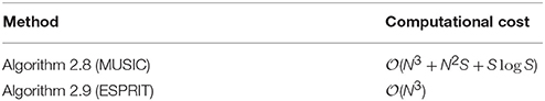
Table 2. Computational costs for the Algorithms 2.8 and 2.9 in the case of N given samples, where S is a large even integer so that all frequencies φ_j are of the form $\frac{{\omega }_j}{S}$ with ${\omega }_j\in (-\frac{S}{2},\frac{S}{2}]\cap \mathbb{Z}$.

3. Sparse Fast Fourier Transform

In this section, we apply Algorithm 2.8 (MUSIC) resp. Algorithm 2.9 (ESPRIT) to the reconstruction of sparse trigonometric polynomials. Clearly, one can approximate the unknown frequencies φ_j of the exponential sum (1.1) by fractions. Therefore, we assume that the unknown frequencies φ_j of (1.1) are fractions $\frac{{\omega }_j}{S}$ with ${\omega }_j\in (-\frac{S}{2},\frac{S}{2}]\cap \mathbb{Z}$, where S is a large even integer. Replacing the variable x by Sx in (1.1), we obtain the new exponential sum (1.2). Then (1.2) is a 1-periodic trigonometric polynomial with sparsity M. Consequently we consider the spectral estimation problem (P2) as mentioned in Section 1. A fast algorithm, which solves the problem (P2) or (P2*), is called sparse fast Fourier transform (sparse FFT). In recent years many sublinear algorithms for sparse FFTs were proposed, see Section 1 and Remark 3.1.

In the following, we propose a new deterministic sparse FFT for solving the problem (P2) of a trigonometric polynomial (1.2) with large sparsity M. Using divide–and–conquer technique, we split the trigonometric polynomial (1.2) of large sparsity M into some trigonometric polynomials of lower sparsity and determine corresponding samples. Here we borrow an idea from sparse FFT in Christlieb et al. [12] and use shifted sampling of (1.2). For a positive integer P ≤ S and a parameter K ∈ ℕ, K ≥ 2, we construct a discrete array of samples of size P×(2K + 1) via

$\begin{array}{ll}{g}_P[s,k]:\text{}=g\left(\frac{s}{P}+\frac{k}{S}\right),(s=0,\dots ,P-1;k=0,\dots ,2K).\hfill & (3.1)\hfill \end{array}$

For each k = 0, …, 2K we form the discrete Fourier transform (DFT) of length P and obtain

$\begin{array}{ll}{\widehat{g}}_P[\ell ,k]:\text{}={\displaystyle \sum _{s=0}^{P-1}{g}_P}[s,k]{\text{e}}^{-2\pi \text{i}s\ell /P}(\ell =0,\dots ,P-1).\hfill & (3.2)\hfill \end{array}$

The fast Fourier transform (FFT) allows the rapid computation of this DFT of length P in ${O}$(P log P) operations. In Figure 1, the sampling scheme and the applied DFTs are visualized. Next, for each ℓ = 0, …, P − 1, it follows that

$\begin{array}{l}{\widehat{g}}_P[\ell ,k]={\displaystyle \sum _{s=0}^{P-1}{\displaystyle \sum _{j=1}^M{c}_j}}{\text{e}}^{2\pi \text{i}{\omega }_j(s/P+k/S)}{\text{e}}^{-2\pi \text{i}s\ell /P}\\ ={\displaystyle \sum _{j=1}^M{c}_j}{\text{e}}^{2\pi \text{i}{\omega }_{j}k/S}\underset{=0\text{or}P}{\underbrace{{\displaystyle \sum _{s=0}^{P-1}{\text{e}}^{2\pi \text{i}({\omega }_j-\ell )s/P}}}}.\end{array}$

FIGURE 1

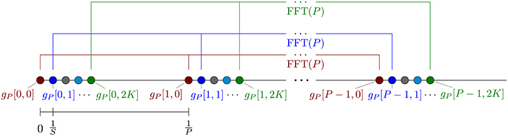
Figure 1. Illustration of the sampling scheme (3.1) and the applied DFTs (3.2).

Now we define the index sets

$I_P(\ell ):\text{}=\{j\in \{1,\dots ,M\}:{\omega }_j\equiv \ell (\text{mod }P)\}$

Such that

${\widehat{g}}_P[\ell ,k]=P{\displaystyle \sum _{j\in I_P(\ell )}{c}_j}{\text{e}}^{2\pi \text{i}{\omega }_{j}k/S}.$

Consequently, for each ℓ = 0, …, P − 1, we may interpret ĝ_P[ℓ, k] (k = 0, …, 2K) as samples of a trigonometric polynomial with frequencies supported only on the index set ${\left\{{\omega }_j\right\}}_{j\in I_P(\ell )}$ ⊂ {ω₁, …, ω_M}, where the samples are taken at the nodes k∕S (k = 0, …, 2K). In simplified terms, the trigonometric polynomial (1.2) is partitioned into P many trigonometric polynomials of smaller sparsity.

Next, we use K ∈ ℕ, K ≥ 2, as sparsity cut-off parameter. This means for each ℓ = 0, …, P − 1, we apply Algorithm 2.8 resp. 2.9 to the “samples” ${\tilde{h}}_k:={ĝ}_P\left[\ell ,k\right]$ (k = 0, …, 2K) and we check if we can uniquely identify all frequencies ω_j, j ∈ I_P(ℓ), i.e., if the determined sparsity M_ℓ: = M from Algorithm 2.8 resp. 2.9 fulfills M_ℓ < K. In this case, we use the obtained local fractions ${\tilde{\phi }}_j$ to compute the frequencies ${\omega }_j=\text{round}({\tilde{\phi }}_{j}S)$ by rounding to nearest integer and we use the corresponding coefficients c_j.

When the condition |I_P(ℓ)| < K is fulfilled for all ℓ = 0, …, P − 1, this approach requires (2K + 1)P samples of g and 2K + 1 FFTs of length P. The computational costs for the corresponding algorithms are listed in Table 3.

TABLE 3

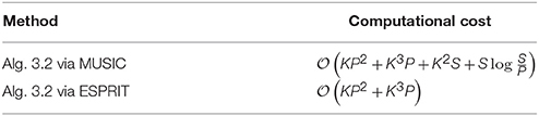
Table 3. Computational cost of one iteration step of Algorithm 3.2 in the case of (2K + 1)P given samples (3.1).

If we cannot uniquely identify all frequencies, i.e., if |I_P(ℓ)| ≥ K for some ℓ, then we form iteratively the new trigonometric polynomial

$\begin{array}{ll}{g}_1(x):\text{}=g(x)-{\displaystyle \sum _{j\in I}{c}_j}{\text{e}}^{2\pi \text{i}{\omega }_{j}x},\hfill & (3.3)\hfill \end{array}$

where I is the union of all I_P(ℓ) with the property |I_P(ℓ)| < K. In the next iteration step, we choose a positive integer P₁ ≤ S different from P and repeat the method on the trigonometric polynomial g₁. In doing so, we can compute the values

$\begin{array}{l}{\displaystyle \sum _{j\in I}{c}_j}{\text{e}}^{2\pi \text{i}{\omega }_j(\frac{s}{P_1}+\frac{k}{S})}={\displaystyle \sum _{j\in I}\left(c_j{\text{e}}^{2\pi \text{i}\frac{{\omega }_j}{P_1}s}\right)}{\text{e}}^{2\pi \text{i}\frac{{\omega }_j}{S}k}\\ (s=0,\dots ,P_1-1;k=0,\dots ,2K)\end{array}$

by the non-equispaced fast Fourier transform (NFFT) [29] in ${O}$(P₁(K logK + |I|)) arithmetic operations.

We perform additional iterations until all frequencies can be identified, i.e., if |I_P1(ℓ)| < K for all ℓ = 0, …, P₁ − 1. Note that our algorithm is related to the sparse FFT proposed in Christlieb et al. [12]. But here we use the methods of Section 2, if aliasing with respect to modulo P occurs.

Remark 3.1 (Relations to other sparse FFTs) In Hassanieh et al. [15], an algorithm for the problem (P2*) is presented, which allows to determine the (unknown) support I and the Fourier coefficients c_j from ${O}$(M log S) samples with computational cost of ${O}$(M log S) operations, as well as a second algorithm, which allows the M-sparse ℓ₂ best approximation of the Fourier coefficients of g from ${O}$(M log(S) log(S∕M)) samples with computational cost of ${O}$(M log(S) log(S∕M)) operations. As mentioned in the introduction, preliminary tests of the implementation [21] suggest that this method may also work for the problem (P2), if an upper bound for the sparsity of the signal is used as sparsity input parameter. In Indyk et al. [30], another variant was discussed, where the number of samples is ${O}$(M logS)(log logS)^${O}$(1) and the computational cost is ${O}$(M log²S)(log logS)^${O}$(1).

Recently in Indyk and Kapralov [31], a result was presented for the multivariate case where the number of required samples is ${O}$(M log S) for constant dimensions d and the computational cost is ${O}$(S^d log ^${O}$(1)S). In general the exact constants, especially the dependence on d, are unknown due to missing implementations. For instance the number of samples ${O}$(M log S) of the last mentioned algorithm contains a factor of d^${O}$(d), see Section [31, Section 4].

Moreover, a deterministic sparse FFT, using the Chinese Remainder Theorem, was presented in [13] for the univariate case and in Iwen [32] for the multivariate case, which takes ${O}$(d⁴M² log⁴(dS)) samples and arithmetic operations. This means there is neither a exponential/super-exponential dependency on the dimension d ∈ ℕ nor a dependency on a failure probability in the asymptotics of the number of samples and arithmetic operations for this method. Besides this deterministic algorithm, there also exists a randomized version which only requires ${O}$(d⁴M log⁴(dS)) samples and arithmetic operations.

Recently, another sparse FFT, which is based on a multiscale approach, was presented in Christlieb et al. [12] as an extension of the method [11]. Their algorithm is able to handle (additive) noise and requires ${O}$(M log(S∕M)) on average.

For further references on the sparse FFT we refer to the nice webpage http://groups.csail.mit.edu/netmit/sFFT/. Despite the fact that the computational cost of the sparse FFT is lower, it is not clear which algorithm is indeed faster and more stable for the practical problems mentioned in the Section 5.

We stress again that it is already well known that one can use Prony-type methods for the sparse FFT, see e.g., Heider et al. [33]. Using the proposed splitting approach, one can significantly decrease the high computational cost of MUSIC and ESPRIT, but keep the numerical stable evaluation. Clearly one can combine the suggested method with a reconstruction of the non-zero Fourier coefficients in a dimension incremental way [34]. □

All of the methods described in Section 2 apply an SVD and use the tolerance ε as a relative threshold parameter to determine the local sparsity M_ℓ of the signal. A good choice of this parameter may depend without limitation on noise in the sampling values of the trigonometric polynomial g and on the smallest distance between two frequencies, where this distance may change for each ℓ ∈ {0, …, P − 1} in each iteration. We propose to use a (small) list of possible relative threshold parameters ε, which are tested for each ℓ ∈ {0, …, P − 1} in each iteration.

Our sparse FFT for recovery of a trigonometric polynomial (1.2) with large sparsity M reads as follows:

Algorithm 3.2 (Sparse FFT via MUSIC resp. ESPRIT, see Algorithm 6.1 for detailed listing with extended parameter list).

Input: S ∈ 2ℕ frequency grid parameter, K ∈ ℕ (K ≥ 2) Hankel matrix size parameter, P ∈ ℕ (P ≤ S) initial FFT length, $\tilde{g}$ 1-periodic sparse trigonometric polynomial (1.2) of unknown sparsity M ∈ ℕ with frequencies in $(-\frac{S}{2},\frac{S}{2}]\cap \mathbb{Z}$ perturbed by noise.

1. For each k = 0, …, 2K, sample ${\tilde{g}}_P\left[s,k\right]:=\tilde{g}\left(\frac{s}{P}+\frac{k}{S}\right)$, s = 0, …, P − 1, and compute ${ĝ}_P\left[\ell ,k\right]{}_{\ell =0}^{P-1}$ by FFT of ${\tilde{g}}_P\left[s,k\right]{}_{s=0}^{P-1}$.

2. for ℓ = 0, …, P − 1

2.1. Apply Algorithm 2.8 resp. 2.9 with L: = K and N: = 2K + 1 on the values ${\tilde{h}}_k:={ĝ}_P\left[\ell ,k\right]{}_{k=0}^{2K}$ to obtain the local sparsity M_ℓ: = M and the local fractions ${\tilde{\phi }}_{\ell ,m}:={\tilde{\phi }}_m\in (-\frac{1}{2},\frac{1}{2}]$ for m = 1, …, M_ℓ. If M_ℓ ≥ K, then go to step 2 and continue with next ℓ. Otherwise, compute the local frequencies ${\omega }_{\ell ,m}:=\text{round}({\tilde{\phi }}_{\ell ,m}S)$ by rounding to nearest integer.

2.2. Compute the local coefficients c_{ℓ, m} as least squares solution of the overdetermined Vandermonde system

$\begin{array}{ll}\begin{array}{l}\underset{{(c_{\ell ,m})}_{m=1}^{M_{\ell }}\in {ℂ}^{M_{\ell }}}{\min }\Vert P{\left({\text{e}}^{2\pi \text{i}k{\omega }_{\ell ,m}/S}\right)}_{k=0,m=1}^{2K,M_{\ell }}\\ {(c_{\ell ,m})}_{m=1}^{M_{\ell }}-{\left({\widehat{g}}_P[\ell ,k]\right)}_{k=0}^{2K}{\Vert }_2.\end{array}\hfill & (3.4)\hfill \end{array}$

2.3. If the residual of (3.4) is small (see step 3.3.6 of Algorithm 6.1), then append the frequencies ω_{ℓ, m} (m = 1, …, M_ℓ) to the frequency set Ω.

3. If the (global) residual

$\underset{\begin{array}{c}s=0,\dots ,P-1\\ k=0,\dots ,2K\end{array}}{\max }|{\displaystyle \sum _{j^{\prime }=1}^{\left|\Omega \right|}C}[j^{\prime }]{\text{e}}^{2\pi \text{i}\Omega [j^{\prime }]\left(\frac{s}{P}+\frac{k}{S}\right)}-g\left(\frac{s}{P}+\frac{k}{S}\right)|$

is small, then exit the algorithm. Otherwise, form the new trigonometric polynomial (3.3). In the next iteration step choose a positive integer P₁ ≤ S different from P, sample (3.3) on $\frac{s}{P_1}+\frac{k}{S}$ for s = 0, …, P₁ − 1 and k = 0, …, 2K, and repeat the above method.

Output: $\Omega \subset (-\frac{S}{2},\frac{S}{2}]\cap \mathbb{Z}$ set of recovered frequencies ω_j (j = 1, …, M), M: = |Ω| detected sparsity, c_j ∈ ℂ coefficient related to ω_j (j = 1, …, M).

For (2K + 1)P given samples (3.1), the computational cost for one iteration of Algorithm 3.2 is shown in Table 3.

If we take (2K + 1)P = ${O}$(M) samples, then we obtain minimal computational cost for the parameters K = ${O}$(M^1∕3) and P = ${O}$(M^2∕3). For this case, we compare the numbers of required samples and computational costs for different methods of spectral estimation in Table 4 such as sparse FFT via MUSIC, sparse FFT via ESPRIT, MUSIC, ESPRIT, and classical FFT. As we can see, the sparse FFT via ESPRIT is very useful for the spectral estimation by a relatively low number of samples and low computational cost.

TABLE 4

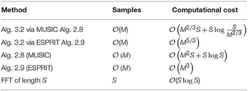
Table 4. Numbers of required samples and computational costs using the splitting approach for one iteration of Algorithm 3.2 as well as for Algorithms 2.8 and 2.9 in the case K = ${O}$(M^1∕3), P = ${O}$(M^2∕3) and M ≈ L∕2 ≈ N∕4.

4. Reconstruction of Multivariate Trigonometric Polynomials

Let d, M ∈ ℕ with d > 1 be given. We consider the d-variate exponential sum of sparsity M

$\begin{array}{ll}g(x):\text{}={\displaystyle \sum _{j=1}^M{c}_j}{\text{e}}^{2\pi \text{i}{\omega }_j·x}\hfill & (4.1)\hfill \end{array}$

for $\mathbf{x}:={(x_1,\dots ,x_d)}^{\text{T}}\in {ℝ}^d$ with non-zero coefficients c_j ∈ ℂ and distinct frequency vectors ${\mathbf{\omega }}_j\in {\mathbb{Z}}^d$. Here the dot in the exponent denotes the usual scalar product in ℝ^d. Note that the function (4.1) is a d-variate trigonometric polynomial of sparsity M which is 1-periodical with respect to each variable. Let Ω: = {ω₁, …, ω_M} be the set of the frequency vectors.

Assume that it is known a priori that ω_j are contained in a frequency set Γ ⊂ ℤ^d. Then the cardinality of Γ satisfies |Γ| ≥ M. Examples of possible frequency sets Γ are the cube $\left\{\mathbf{k}\in {\mathbb{Z}}^d:\left|\right|\mathbf{k}|{|}_{\infty }\le N\right\}$ and the symmetric hyperbolic cross

$\left\{k={(k_s)}_{s=1}^d\in {\mathbb{Z}}^d:{\displaystyle \prod _{s=1}^d\max }\{1,|k_s|\}\le N\right\}.$

For given z ∈ ℤ^d and S ∈ ℕ, the set

$\Lambda (z,S):\text{}=\left\{x_k=\frac{k}{S}z\text{mod}1;k=0,\dots ,S-1\right\}\subset {𝕋}^d\simeq {\left[0,1\right)}^d$

is called rank–1 lattice, where 1: = (1, …, 1)^T. Note that x_k = x_k+nS for k = 0, …, S − 1 and n ∈ ℤ. For given Γ ⊂ ℤ^d, there exists a reconstructing rank-1 lattice Λ(z, S) such that the matrix

$A_{S,\left|\Gamma \right|}:\text{}={({\text{e}}^{2\pi \text{i}k·x})}_{x\in \Lambda (z,S),k\in \Gamma }$

fulfills the condition (see [35] and [36, Section 3.2])

$\begin{array}{ll}{A}_{S,\left|\Gamma \right|}^{\ast }{A}_{S,\left|\Gamma \right|}=S{I}_{\left|\Gamma \right|}.\hfill & (4.2)\hfill \end{array}$

Then we consider the following spectral estimation problem:

(P3) Assume that ω_j ∈ Γ (j = 1, …, M) and that Λ(z, S) is a reconstructing rank–1 lattice with respect to Γ. Recover the sparsity M ∈ ℕ, all frequencies ω_j ∈ Γ as well as all non-zero coefficients c_j ∈ ℂ of the d-variate exponential sum (4.1), if noisy sampled data

${\tilde{g}}_k:\text{}=g(x_k)+e_k\left(|e_k|\le \frac{1}{10}{\min }_j|c_j|\right)$

for all k = 0, …, 2L − 2 are given, where x_k ∈ Λ(z, S), S ≥ L > M and e_k ∈ ℂ are small error terms.

For simplicity we discuss only noiseless data. Let $H_L:={(g(x_{k+n}))}_{k,n=0}^{L-1}$ be the response matrix of the given data. Then H_L is a Hankel matrix. Further we introduce the rectangular Fourier-type matrix

$F_{L,M}:\text{}={({\text{e}}^{2\pi \text{i}{\omega }_j·x_k})}_{k=0,j=1}^{L-1,M}.$

From (4.2) it follows in the case L = S that ${\mathbf{F}}_{S,M}^{*}{\mathbf{F}}_{S,M}=S{\mathbf{I}}_M$ and hence for all x ∈ ℂ^M

$\Vert F_{S,M}x{\Vert }_2^2=x^{\ast }{F}_{S,M}^{\ast }{F}_{S,M}x=S\Vert x{\Vert }_2^2.$

Consequently, all positive singular values of F_{S, M} are equal to $\sqrt{S}$ and cond₂F_{S, M} = 1.

The matrix H_L can be represented in the form

$\begin{array}{ll}{H}_L=F_{L,M}(\text{diag}{(c_j)}_{j=1}^M)F_{L,M}^{\text{T}}.\hfill & (4.3)\hfill \end{array}$

The ranges of H_L and F_{L, M} coincide in the noiseless case by (4.3). The range of F_{L, M} is a proper subspace of ℂ^L. This subspace is called left signal space ${S}$_L. The left signal space ${S}$_L is of dimension M and is generated by the M columns e_L(ω_j) (j = 1, …, M), where

$e_L(\omega ):\text{}={({\text{e}}^{2\pi \text{i}\omega ·x_k})}_{k=0}^{L-1}(\omega \in \Gamma ).$

Note that $\left|\right|{\mathbf{e}}_L(\mathbf{\omega })|{|}_2=\sqrt{L}$ for each ω ∈ Γ. The left noise space ${N}$_L is defined as the orthogonal complement of ${S}$_L in ℂ^L. The dimension of ${N}$_L is equal to L − M > 0.

By Q_L we denote the orthogonal projection onto the left noise space ${N}$_L. Since e_L(ω_j) ∈ ${S}$_L (j = 1, …, M) and ${N}$_L⊥${S}$_L, we obtain that

$Q_L{e}_L({\omega }_j)=0(j=1,\dots ,M).$

If ω ∈ Γ \ Ω, then the vectors ${\mathbf{e}}_L({\mathbf{\omega }}_1),\dots ,{\mathbf{e}}_L({\mathbf{\omega }}_M),{\mathbf{e}}_L(\mathbf{\omega })\in {ℂ}^L$ are linearly independent for S ≥ L > M. This can be seen as follows: For distinct ω, ω′ ∈ Γ, it follows by [36, Lemma 3.1] that

$\omega ·z\cancel{\equiv }\omega \prime ·z(\text{mod}S).$

Consequently the vectors

$e_L({\omega }_j):\text{}={({\text{e}}^{2\pi \text{i}({\omega }_j·z)\frac{k}{S}})}_{k=0}^{L-1}(j=1,\dots ,M)$

and e_L(ω) with ω ∈ Γ \ Ω are linearly independent for S ≥ L > M, since the square Vandermonde matrix

$(e_L({\omega }_1)|\dots |e_L({\omega }_M)|e_L(\omega ))(1:M+1,1:M+1)$

is invertible for each L ≥ M + 1. Hence

$e_L(\omega )\notin S_L=\text{span}\{e_L({\omega }_1),\dots ,e_L({\omega }_M)\},$

i.e. Q_Le_L(ω) ≠ 0.

Thus, the frequency vectors can be determined via the M zeros resp. lowest local minima of the left noise-space correlation function

$N_L(\omega ):\text{}=\frac{1}{\sqrt{L}}\Vert Q_L{e}_L(\omega ){\Vert }_2(\omega \in \Gamma )$

or via the M peaks of the left imaging function

$J_L(\omega ):\text{}=\sqrt{L}\Vert Q_L{e}_L(\omega ){\Vert }_2^{-1}(\omega \in \Gamma ).$

Similar to Section 2, one can determine the left noise-space correlation function resp. the left imaging function on Γ by using SVD of the response matrix H_L.

Now, we proceed analogously to Section 3. For a positive integer P ≤ S and a parameter K ∈ ℕ, K ≥ 2, we construct the sampling array of (4.1) of size P × (2K + 1) via

$g_P[s,k]:\text{}=g\left(\left(\frac{s}{P}+\frac{k}{S}\right)z\right)(s=0,\dots ,P-1;k=0,\dots ,2K).$

As in the univariate case, for each k = 0, …, 2K we form the DFT of length P

${\widehat{g}}_P[\ell ,k]:\text{}={\displaystyle \sum _{s=0}^{P-1}{g}_P}[s,k]{\text{e}}^{-2\pi \text{i}s\ell /P}(\ell =0,\dots ,P-1).$

For each ℓ = 0, …, P − 1, we obtain that

$\begin{array}{l}{\widehat{g}}_P[\ell ,k]={\displaystyle \sum _{s=0}^{P-1}{\displaystyle \sum _{j=1}^M{c}_j}}{\text{e}}^{2\pi \text{i}(s/P+k/S){\omega }_j·z}{\text{e}}^{-2\pi \text{i}s\ell /P}\\ ={\displaystyle \sum _{j=1}^M{c}_j}{\text{e}}^{2\pi \text{i}k{\omega }_j·z/S}{\displaystyle \sum _{s=0}^{P-1}{\text{e}}^{2\pi \text{i}(({\omega }_j·z)-\ell )s/P}}.\end{array}$

Introducing the index sets

$I_P(\ell ):\text{}=\{j\in \{1,\dots ,M\}:{\omega }_j·z\equiv \ell (\text{mod}P)\}(\ell =0,\dots ,P-1),$

it follows that

${\widehat{g}}_P[\ell ,k]=P{\displaystyle \sum _{j\in I_P(\ell )}{c}_j}{\text{e}}^{2\pi \text{i}k{\omega }_j·z/S}.$

This means for each ℓ = 0, …, P − 1, we may interpret ĝ_P[ℓ, k] (k = 0, …, 2K) as samples of a multivariate trigonometric polynomial with frequencies supported on the index set {ω_j}_{j ∈ IP(ℓ)} ⊂ {ω₁, …, ω_M}, where the samples are taken at the nodes $\frac{k}{S}\mathbf{z}$ (k = 0, …, 2K). In Figure 2, a two-dimensional example is shown which visualizes the partitioning by the index sets I_P(ℓ).

FIGURE 2

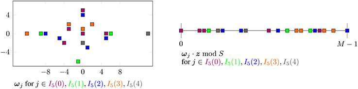
Figure 2. Illustration of an example frequency index set ${\left\{{\mathbf{\omega }}_j\right\}}_{j=1}^{19}$ and corresponding one-dimensional frequencies ω_j · z mod S partitioned by I_P(ℓ) with parameters P: = 5, z: = (1, 33)^T, S: = 37.

Next, we apply Algorithm 2.8 resp. 2.9 with L: = K and N: = 2K + 1 on the values ${\tilde{h}}_k:={ĝ}_P\left[\ell ,k\right]$ (k = 0, …, 2K) for each ℓ = 0, …, P − 1 to obtain the local sparsity M_ℓ = M and the local fractions ${\tilde{\phi }}_{\ell ,m}:={\tilde{\phi }}_m\in (-\frac{1}{2},\frac{1}{2}]$ for m = 1, …, M_ℓ. Afterwards, we compute the one-dimensional frequencies ${\omega }_{\ell ,m}:=\text{round}({\tilde{\phi }}_{\ell ,m}S)\in (-\frac{S}{2},\frac{S}{2}]\cap \mathbb{Z}$ by rounding to nearest integer. We transform these one-dimensional frequencies ω_{ℓ, m} into their d-dimensional counterparts ω_{ℓ, m} ∈ Γ using the relation ω_{ℓ, m} · z ≡ ω_{ℓ, m} (mod S) given by the reconstructing rank-1 lattice Λ(z, S). Then we compute coefficients c_{ℓ, m} from the samples ĝ_P[ℓ, k] (k = 0, …, 2K) by solving the corresponding overdetermined Vandermonde system. If we cannot identify all the frequencies, i.e., if |I_P(ℓ)| ≥ K for some indices ℓ, we consider the new trigonometric polynomial

$\begin{array}{ll}\begin{array}{l}{g}_1(x):=g(x)-{\displaystyle \sum _{j\in I}{c}_j}{\text{e}}^{2\pi \text{i}{\omega }_j·x}={\displaystyle \sum _{j=1}^M{c}_j}{\text{e}}^{2\pi \text{i}{\omega }_j·x}-{\displaystyle \sum _{j\in I}{c}_j}{\text{e}}^{2\pi \text{i}{\omega }_j·x}\\ (x\in {𝕋}^d)\end{array}\hfill & (4.4)\hfill \end{array}$

in an additional iteration, where the index set I contains all index sets I_P(ℓ) with |I_P(ℓ)| < K. In the next iteration, we choose a positive integer P₁ ≤ S different from P and repeat the method for the trigonometric polynomial g₁. In doing so, we compute the values

$\begin{array}{l}{\displaystyle \sum _{j\in I}{c}_j}{\text{e}}^{2\pi \text{i}(\frac{s}{P_1}+\frac{k}{S}){\omega }_j·z}={\displaystyle \sum _{j\in I}\left(c_j{\text{e}}^{2\pi \text{i}\frac{{\omega }_j}{P_1}s}\right)}{\text{e}}^{2\pi \text{i}\frac{{\omega }_j·z}{S}k}\\ (s=0,\dots ,P_1-1;k=0,\dots ,2K)\end{array}$

of the second sum in (4.4) evaluated at the nodes $\mathbf{x}=(\frac{s}{P_1}+\frac{k}{S})\mathbf{z}$ with the univariate NFFT [29] in ${O}$(P₁(K log K + |I|)) arithmetic operations. We perform additional iterations until all frequencies can be identified, i.e. |I_P1(ℓ)| < K for all ℓ = 0, …, P₁ − 1.

We modify Algorithm 3.2 from Section 3 as described above and additionally in the following way. Here, we describe the changes in the detailed listing (see Algorithm 6.1) of Algorithm 3.2. In step 1, we sample the multivariate trigonometric polynomial at the nodes $\left(\frac{s}{P}+\frac{k}{S}\right)·\mathbf{z}(s=0,\dots ,P-1,k=0,\dots ,2K)$. In step 3.3.3, we compute the local frequencies ${\omega }_{\ell ,m}:=round({\tilde{\phi }}_{\ell ,m}S)$ for m = 1, …, M_ℓ. Next, we compute the d-dimensional counterparts ω_{ℓ, m} of the one-dimensional frequencies ω_{ℓ, m} using the relation ω_{ℓ, m} · z ≡ ω_{ℓ, m} (mod S). In step 3.3.4, we filter the frequencies ω_{ℓ, m} by removing non-unique ones and by keeping only those with ω_{ℓ, m} · z ≡ ℓ(mod P). We remark that we have to modify step 3.3.4 and that we have to perform the conversion of one-dimensional frequencies ω_{ℓ, m} to their d-dimensional counterparts ω_{ℓ, m} before the filtering, since the conditions ω_{ℓ, m} · z ≡ ℓ(mod P) and ω_{ℓ, m} ≡ ℓ(mod P) are not equivalent in general if P is not a divisor of S.

5. Numerical Experiments

In this section, we present some numerical results for Algorithm 3.2. The related software is available from the authors' homepage. All computations are performed in MATLAB with IEEE double–precision arithmetic. First we consider noiseless sampled data and later the case, where the sampled data are perturbed by additive (white) Gaussian noise. Finally we present some numerical results for the modified Algorithm 3.2 of Section 4.

5.1. Noiseless Sampled Data

Example 5.1 From noiseless sampled values, we reconstruct 100 trigonometric polynomials (1.2) of sparsity M = 256 with random frequencies ${\omega }_j\in (-\frac{S}{2},\frac{S}{2}]\cap \mathbb{Z}$ and random coefficients c_j on the unit circle. We set the array of relative SVD threshold values epsilon_svd_list: = [10⁻³, 10⁻⁴, …, 10⁻⁸], the parameter ${\epsilon }_{\text{spatial}}:=10^{-8}$, the absolute value of minimal non-zero coefficients ${\epsilon }_{\text{fc}\_\text{min}}:=10^{-1}=10^{-1}·\underset{j}{min}|c_j|$ and the maximal number of iterations R: = 10, see Algorithm 6.1 for the extended parameter list. Applying the sparse FFT Algorithm 3.2 with MUSIC in the case S = 2¹⁶ with parameters K ∈ {6, 12, 16} and P ∈ {16, 32, 64, 128}, we can successfully detect all integer frequencies ω_j. In Table 5, the column “iterations” depicts the maximal number of iterations actually used by the Algorithm 3.2 (computed over 100 trigonometric polynomials). The column “samples” contains the maximal number of sampled values used by the Algorithm 3.2. The column “ℓ²–errors” shows the maximal relative ℓ²–error of the coefficients, which are locally computed in step 2.2 of Algorithm 3.2. The column “updated ℓ²–errors” shows the maximal relative ℓ²–error of the coefficients, which are determined by additionally solving one large Vandermonde system at the end of Algorithm 3.2 with all frequencies as well as all samples of (1.2). For comparison, the classical FFT of length 2¹⁶ requires 2¹⁶ samples and the resulting ℓ²–error is 2.6e-16. The minimal number of samples for the cases K ∈ {6, 12, 16} and P ∈ {16, 32, 64, 128} is reached for K = P = 16 with 1716 samples, the next smallest number of samples is 1725 for K = 12 and P = 32. If we do not use the splitting approach (P = 1 and R = 1), we observe that the detection of some frequencies fails for exactly 1 of the 100 signals for K = 750 and the detection of all frequencies of all 100 signals succeeds for K = 850 requiring 1701 samples. This number of samples is very close to the minimum of 1716 samples from above. However, a direct application of MUSIC method (entry K = 850) has distinctly more computational cost than using the sparse FFT Algorithm 3.2. Note that R denotes the maximal number of iterations in Algorithm 6.1, the detailed description of Algorithm 3.2. □

TABLE 5

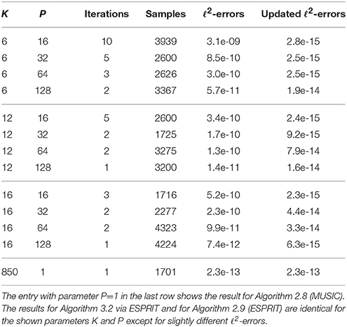
Table 5. Results for Algorithm 3.2 via MUSIC for frequency grid parameter S = 2¹⁶ and sparsity M = 256 with random coefficients on the unit circle.

Example 5.2 Now we apply Algorithm 3.2 via ESPRIT with the same parameters as in Example 5.1. Then we obtain identical results for the number of iterations and samples as well as almost identical ℓ²-errors, but Algorithm 3.2 via ESPRIT has lower computational cost. If we do not use the splitting approach (P = 1 and R = 1), we observe that the detection of some frequencies fails for exactly 2 of the 100 signals for K = 750 and the detection of all frequencies of all 100 signals again succeeds for K = 850 requiring 1701 samples.

Additionally, we apply the implementation [21] of the sfft version 3 algorithm. The number of used samples is 7669, which is about two to four times the number of samples for the MUSIC and ESPRIT algorithm in Table 5, and the maximal relative ℓ²-error of the coefficients is 3.6e-04, which is about five orders of magnitude larger. □

Example 5.3 We generate 100 random trigonometric polynomials (1.2), where the coefficients c_j are drawn uniformly at random from [−1, 1] + [−1, 1]i with $|c_j|\ge 10^{-2}$. We set the absolute value of minimal non-zero coefficients ${\epsilon }_{\text{fc}\_\text{min}}:=10^{-3}=10^{-1}·\underset{j}{min}|c_j|$. For the cases K ∈ {6, 12, 16} and P ∈ {16, 32, 64, 128}, we apply Algorithm 3.2 via ESPRIT. We obtain results almost identical to the ones from Example 5.2. This means, all frequencies of all 100 signals are correctly detected and the maximal relative ℓ²-errors differ slightly from those in Table 5. The maximal numbers of iterations and samples are identical.

Additionally, we apply the implementation [21] of the sfft version 3 algorithm. For each signal, the number of taken samples is 7669. Only for 16 of the 100 signals, all frequencies are detected correctly, whereas between 1 and 7 frequencies are not correctly detected for 84 signals. □

Example 5.4 Next we apply Algorithm 3.2 via ESPRIT for signals with higher sparsity. From noiseless sampled values, we reconstruct 100 trigonometric polynomials (1.2) of sparsity M = 1024 with random frequencies ${\omega }_j\in (-\frac{S}{2},\frac{S}{2}]\cap \mathbb{Z}$ and random coefficients c_j on the unit circle. The results for the frequency grid parameter S: = 2²² are shown in Table 6. The minimal number of samples is about six times higher compared to the results in Table 5.

In general, we observe that the maximal number of used iterations decreases for increasing initial FFT length P ∈ {64, 128, 256, 512} as well as for increasing values K ∈ {8, 10, 12}. In the cases, where all frequencies of all the 100 trigonometric polynomials are correctly detected, the number of required samples first decreases and later increases again for increasing initial FFT length P and fixed values K. The reason for this is that the number of samples per iteration increases for growing FFT length, while the number of used iterations decreases until its minimum one is reached.

Again, we apply the implementation [21] of the sfft version 3 algorithm. Here, the number of used samples is 31718, which is up to three times the number of samples of Algorithm 3.2 via ESPRIT in Table 6, and the maximal relative ℓ²-error of the coefficients is 3.6e-04, which is about five orders of magnitude larger than in Table 6. □

TABLE 6

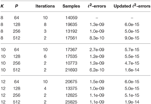
Table 6. Results for Algorithm 3.2 via ESPRIT for frequency grid parameter S = 2²² and sparsity M = 1024 with random coefficients on the unit circle.

5.2. Noisy Case

In this subsection, we test the robustness to noise of Algorithm 3.2. For this, we perturb the samples of the trigonometric polynomials g from (1.2) by additive complex white Gaussian noise with zero mean and standard deviation σ, i.e., we have measurements $\tilde{g}\left(\frac{k}{S}+\frac{s}{P}\right)=g(\frac{k}{S}+\frac{s}{P})+{\eta }_{k,s}$, where η_{k, s} ∈ ℂ are independent and identically distributed complex Gaussian noise values. Then, we may approximately compute the signal-to-noise ratio (SNR) in our case by

$\text{SNR}\approx \frac{\frac{1}{S}{\displaystyle {\sum }_{k=0}^{S-1}|g(\frac{k}{S}){|}^2}}{\frac{1}{S}{\displaystyle {\sum }_{k=0}^{S-1}|{\eta }_{k,0}{|}^2}}\approx \frac{{\displaystyle {\sum }_{j=1}^M|c_j{|}^2}}{{\sigma }^2}.$

Correspondingly, we choose $\sigma =\parallel {(c_j)}_{j=1}^M{\parallel }_2∕\sqrt{\text{SNR}}$ for a targeted SNR value. For the numerical computations in MATLAB, we generate the noise by ${\eta }_{k,s}:=\sigma ∕\sqrt{2}$ *(randn + 1i*randn). Moreover, we choose the parameter ε_spatial: = 5σ and this means that the absolute value of the noise |η_{k, s}| ≤ ε_spatial for more than 99.9998% of the noise values η_{k, s}. Since we assume that the absolute value of the noise $\le \frac{1}{10}\underset{j}{min}|c_j|$ throughout this paper, we should choose the SNR such that $5\sigma =5\parallel {(c_j)}_{j=1}^M{\parallel }_2∕\sqrt{\text{SNR}}\le \frac{1}{10}\underset{j}{min}|c_j|$, which yields $\text{SNR}\ge 50^2\parallel {(c_j)}_{j=1}^M{\parallel }_2^2∕{(\underset{j}{min}|c_j|)}^2$.

Example 5.5 As in Example 5.1, we generate 100 trigonometric polynomials (1.2) of sparsity M = 256 with random frequencies ${\omega }_j\in (-\frac{S}{2},\frac{S}{2}]\cap \mathbb{Z}$ and random coefficients c_j from the unit circle. We set the frequency grid parameter S = 2¹⁶, the signal sparsity M = 256, the array of relative SVD threshold values epsilon_svd_list: = [10⁻³, 10⁻⁴, …, 10⁻⁸] and the maximal number of iterations R: = 10. Here, we set the absolute value of minimal non-zero coefficients ${\epsilon }_{\text{fc}\_\text{min}}:=10^{-1}=10^{-1}·\underset{j}{min}|c_j|$ and we use the parameters P ∈ {32, 64, 128} and K ∈ {12, 24}. For possible SNR values, we have $\text{SNR}\ge 50\parallel {(c_j)}_{j=1}^M{\parallel }_2^2∕{(\underset{j}{min}|c_j|)}^2=6.4·10^5$ and we consider the SNR values 10¹⁰, 10⁸, and 10⁶ in our numerical tests. The results of Algorithm 3.2 via ESPRIT are presented in Table 7. Additionally, we test the sparsity cut-off parameter K₂ ∈ ℕ differently from the Hankel matrix size parameter K, see Algorithm 6.1. Here, we use the parameter combinations (K, K₂) ∈ {(12, 6), (12, 12), (24, 12)}. In general, we observe that we require more samples for SNR = 10⁶ than for SNR = 10⁸ and again more for SNR = 10⁸ than for SNR = 10¹⁰. The relative errors are about one order of magnitude larger for SNR = 10⁶ than for SNR = 10⁸ as well as for SNR = 10⁸ than for SNR = 10¹⁰, since the maximal noise values η_{k, s} are larger by about one order of magnitude with high probability each time. Moreover, the maximal number of samples in the noisy case is higher than in the noiseless case, cf. Table 5. For some parameter combinations at SNR = 10⁸, exactly one of the 100 signals is not correctly detected and this is indicated by the entry “–” in the column “ℓ²-errors” resp. “updated ℓ²-errors.” For SNR = 10⁶ with K = 12, K₂ = 6, and P = 64 exactly one frequency at three of the 100 signals is not correctly detected, whereas all frequencies of all 100 signals for SNR = 10⁶ are correctly detected in the other cases shown in Table 7. All parameters of (1.2) are correctly detected in the case SNR = 10¹⁰ for the parameter combinations (K, K₂) ∈ {(12, 6), (12, 12), (24, 12)} and P = 32. For the considered test parameters, the choices (K, K₂) ∈ {(12, 6), (24, 12)}, which yield a higher oversampling within the ESPRIT algorithm, give slightly better results compared to the choice K = K₂ = 12.

TABLE 7

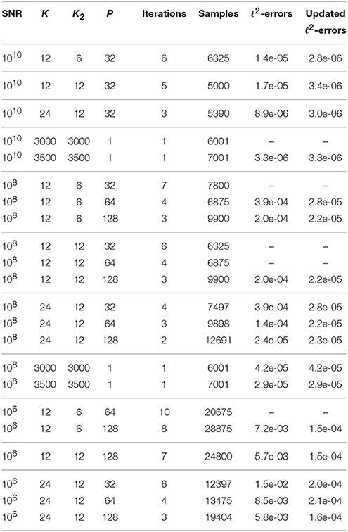
Table 7. Results for Algorithm 3.2 via ESPRIT for frequency grid parameter S = 2¹⁶ and sparsity M = 256 with noisy data.

Additionally, we apply the implementation [21] of the sfft version 3 algorithm. We remark that this particular algorithm is not suited for noisy samples. The number of taken samples is 7669 for all signals, which is about 50 percent higher than for Algorithm 3.2 at SNR = 10¹⁰ and similar at SNR = 10⁸. In the cases SNR = 10¹⁰ and SNR = 10⁸, all frequencies of all 100 signals are correctly detected and the maximal relative ℓ²-errors of the Fourier coefficients are about 3.6e-04. For SNR = 10⁶, all frequencies of 94 of the 100 signals are correctly detected and up to four frequencies at four of the 100 signals are not correctly detected. □

Example 5.6 Additionally, we generate 100 random trigonometric polynomials (1.2), where the coefficients c_j are drawn uniformly at random from [−1, 1] + [−1, 1]i with $\left|c_j\right|\ge 10^{-2}$. We set the absolute value of minimal non-zero coefficients ${\epsilon }_{\text{fc}\_\text{min}}:=10^{-3}=10^{-1}·\underset{j}{min}|c_j|$. In the case SNR = 10⁸, we observe in each considered parameter combination that the correct detection of one or two frequencies fails for several of the 100 trigonometric polynomials. The most likely reason is the fact that the smallest coefficient can be very close to the noise level. If we decrease the noise by one order of magnitude, i.e. SNR = 10¹⁰, the frequency detection succeeds for all considered parameter combinations.

Furthermore, we generate 100 random trigonometric polynomials (1.2), where the coefficients c_j are drawn uniformly at random from [−1, 1] + [−1, 1]i with $\left|c_j\right|\ge 10^{-1}$. Then we set the absolute value of minimal non-zero coefficients ${\epsilon }_{\text{fc}\_\text{min}}:=10^{-2}=10^{-1}·\underset{j}{min}|c_j|$. This means that the smallest possible coefficient as well as the parameter ε_{fc_min} are by one order of magnitude larger than before. Now in both of the cases SNR = 10¹⁰ and SNR = 10⁸, we observe for each parameter combination (K, K₂) ∈ {(12, 6), (12, 12), (24, 12)} and P ∈ {32, 64, 128} that all frequencies of all trigonometric polynomials are correctly detected.

For results of the implementation [21] of the sfft version 3 algorithm, we refer to Example 5.3. □

5.3. Reconstruction of 6-variate Trigonometric Polynomials

Finally we test the modified Algorithm 3.2 of Section 4 for the reconstruction of six-variate trigonometric polynomials with the sparsity M = 256.

Example 5.7 We choose the index set Γ of possible frequency vectors as the six-dimensional hyperbolic cross $\Gamma :=\left\{\mathbf{k}\in {\mathbb{Z}}^6:{\prod }_{s=1}^{6}max\left\{1,\left|k_s\right|\right\}\le 16\right\}$ of cardinality 169209. Further we use the reconstructing rank-1 lattice Λ(z, S) with generating vector z = (1, 33, 579, 3628, 21944, 169230)^T and rank-1 lattice size S = 1105193, see Kämmerer et al. [37, Table 6.2]. We generate 100 random trigonometric polynomials (4.1) with sparsity M = 256, where the frequency vectors ω_j (j = 1, …, M) are chosen uniformly at random from Γ (without repetition) and the corresponding coefficients c_j are randomly chosen on the unit circle. We set the array of relative SVD threshold values epsilon_svd_list: = [10⁻³, 10⁻⁴, …, 10⁻⁸], the absolute value of minimal non-zero coefficients ${\epsilon }_{\text{f}\_\text{min}}:=10^{-1}$, and the maximal number of iterations R: = 10. In the noiseless case, we set the parameter ${\epsilon }_{\text{spatial}}:=10^{-8}$, and in the noisy case as described in Section 5.2. The results of the modified Algorithm 3.2 via ESPRIT are presented in Table 8.

TABLE 8

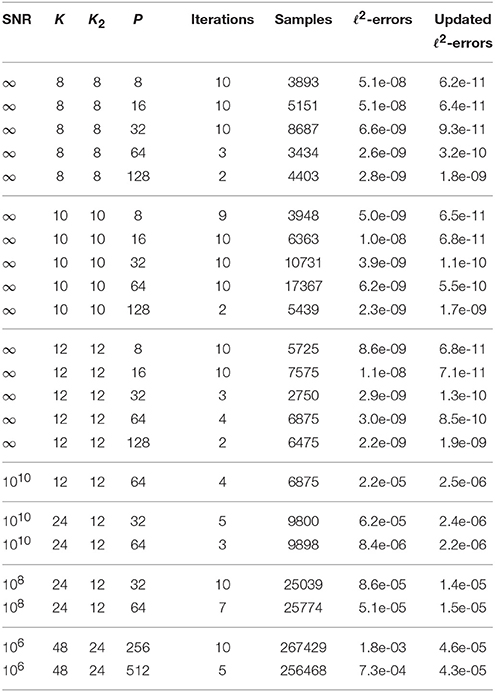
Table 8. Results of the modified Algorithm 3.2 via ESPRIT with sparsity M = 256, frequency vectors within six-dimensional hyperbolic cross index set $\Gamma =\left\{\mathbf{k}\in {\mathbb{Z}}^6:{\prod }_{s=1}^{6}max\left\{1,\left|k_s\right|\right\}\le 16\right\}$, and reconstructing rank-1 lattice Λ(z, S) with z = (1, 33, 579, 3628, 21944, 169230)^T and S = 1105193.

The columns of Table 8 have the same meaning as in Section 5.2. For the noiseless case, i.e., “SNR = ∞,” we observe the same behavior as in the one-dimensional case in Section 5.1. The detection of all frequency vectors of all 100 trigonometric polynomials (4.1) succeeds for K = K₂ ∈ {8, 10, 12} and P ∈ {8, 16, 32, 64, 128}. For the noisy case, the results are worse than in Table 7 of the one-dimensional case. The reason for this is that we have a bijective mapping between six-dimensional ω_j and one-dimensional frequencies ω_j by means of the reconstructing rank-1 lattice, ω_j · z ≡ ω_j(modS), and the rank-1 lattice size S influences how close two distinct one-dimensional fractional frequencies ${\omega }_j^{\prime }∕S$ and ${\omega }_j^{″}∕S$ may get in the ESPRIT algorithm, see also Figure 2.

We tried to apply the implementation [21] of the sfft version 3 algorithm in this test setting. However, the implementation failed with an internal error caused by the used problem size n = S = 1105193 and sparsity M = 256. Another test run with rank-1 lattice size S = 2²¹ = 2097152 yielded 7938 samples and a maximal relative ℓ²-error of 6.8e-04, where the latter is about 4 orders of magnitude larger than the results in Table 8. Moreover, we consider the noisy case. Again, we remark that the implementation [21] is not suited for noisy samples. For SNR = 10¹⁰, the detection of one frequency fails for one of the 100 signals. If we increase the SNR to 10⁸, then between one and 9 frequencies are not correctly detected for 81 of the 100 signals. □

Conflict of Interest Statement

The authors declare that the research was conducted in the absence of any commercial or financial relationships that could be construed as a potential conflict of interest.

Acknowledgments

The first and last named author gratefully acknowledge the funding by the European Union and the Free State of Saxony (EFRE/ESF NBest-SF). The results of this paper were first presented during the Dagstuhl Seminar 15251 on “Sparse modeling and multi-exponential analysis” (June 14 – 19, 2015). Moreover, the authors would like to thank the referees for their valuable suggestions.

References

1. Manolakis DG, Ingle VK, Kogon SM. Statistical and Adaptive Signal Processing. Boston, MA: McGraw-Hill (2005).

Google Scholar

2. Stoica PG, Moses RL. Spectral Analysis of Signals. Upper Saddle River, NJ: Prentice Hall (2005).

Google Scholar

3. Plonka G, Tasche M. Prony methods for recovery of structured functions. GAMM–Mitt. (2014) 37:239–58. doi: 10.1002/gamm.201410011

CrossRef Full Text | Google Scholar

4. Schmidt RO. Multiple emitter location and signal parameter estimation. IEEE Trans Antennas Propag. (1986) 34:276–80.

Google Scholar

5. Roy R, Kailath T. ESPRIT—estimation of signal parameters via rotational invariance techniques. IEEE Trans Acoustic Speech Signal Process. (1989) 37:984–94.

Google Scholar

6. Hua Y, Sarkar TK. Matrix pencil method for estimating parameters of exponentially damped/undamped sinusoids in noise. IEEE Trans Acoust Speech Signal Process. (1990) 38:814–24.

Google Scholar

7. Golub GH, Milanfar P, Varah J. A stable numerical method for inverting shape from moments. SIAM J Sci Comput. (1999) 21:1222–43.

Google Scholar

8. Roy R, Kailath T. ESPRIT—estimation of signal parameters via rotational invariance techniques. In: Auslander L, Grünbaum FA, Helton JW, Kailath T, Khargoneka P, Mitter S, editors. Signal Processing, Part II. Vol. 23 of IMA Volumes in Mathematics and its Applications. New York, NY: Springer (1990). pp. 369–411.

9. Potts D, Tasche M. Parameter estimation for nonincreasing exponential sums by Prony-like methods. Linear Algebra Appl. (2013) 439:1024–39. doi: 10.1016/j.laa.2012.10.036

CrossRef Full Text | Google Scholar

10. Pereyra V, Scherer G. Exponential data fitting. In: Pereyra V, Scherer G, editors. Exponential Data Fitting and its Applications. Sharjah: Bentham Science Publishers; IEEE Computer Society (2010). pp. 1–26.

Google Scholar

11. Lawlor D, Wang Y, Christlieb A. Adaptive sub-linear time Fourier algorithms. Adv Adapt Data Anal. (2013) 5:25. doi: 10.1142/S1793536913500039

CrossRef Full Text | Google Scholar

12. Christlieb A, Lawlor D, Wang. A multiscale sub-linear time Fourier algorithm for noisy data. Appl Comput Harmon Anal. (in press). doi: 10.1016/j.acha.2015.04.002

CrossRef Full Text

13. Iwen MA. Combinatorial sublinear-time Fourier algorithms. Found Comput Math. (2010) 10:303–38. doi: 10.1007/s10208-009-9057-1

CrossRef Full Text | Google Scholar

14. Ben-Or M, Tiwari P. A deterministic algorithm for sparse multivariate polynomial interpolation. In: Twentieth Annual ACM Symposium on the Theory of Computing. New York, NY: ACM Press (1988). pp. 301–9.

15. Hassanieh H, Indyk P, Katabi D, Price E. Nearly optimal sparse Fourier transform. In: Proceedings of the Forty-fourth Annual ACM Symposium on Theory of Computing. New York, NY: ACM (2012). pp. 563–78.

16. Gilbert AC, Indyk P, Iwen M, Schmidt L. Recent developments in the sparse Fourier transform: a compressed Fourier transform for big data. IEEE Signal Proc Mag. (2014) 31:91–100. doi: 10.1109/MSP.2014.2329131

CrossRef Full Text | Google Scholar

17. Rauhut H. Random sampling of sparse trigonometric polynomials. Appl Comput Harmon Anal. (2007) 22:16–42. doi: 10.1016/j.acha.2006.05.002

CrossRef Full Text | Google Scholar

18. Kunis S, Rauhut H. Random sampling of sparse trigonometric polynomials II, orthogonal matching pursuit versus basis pursuit. Found Comput Math. (2008) 8:737–63. doi: 10.1007/s10208-007-9005-x

CrossRef Full Text | Google Scholar

19. Gröchenig K, Pötscher BM, Rauhut H. Learning trigonometric polynomials from random samples and exponential inequalities for eigenvalues of random matrices. arXiv:math/0701781v2. (2010).

Google Scholar

20. Foucart S, Rauhut H. A mathematical introduction to compressive sensing. In: Applied and Numerical Harmonic Analysis. New York, NY: Birkhäuser;Springer (2013).

Google Scholar

21. Schumacher J. sFFT 0.1.0 (2013). Available online at: http://spiral.net/software/sfft.html.

22. Schumacher J, Püschel M. High-performance sparse fast Fourier transforms. In: Proceedings of IEEE Workshop on Signal Processing Systems (SIPS). Belfast, UK: IEEE (2014). pp. 1–6.

23. Liao W, Fannjiang A. MUSIC for single-snapshot spectral estimation: stability and super-resolution. Appl Comput Harmon Anal. (2016) 40:33–67. doi: 10.1016/j.acha.2014.12.003

CrossRef Full Text | Google Scholar

24. Peter T, Potts D, Tasche M. Nonlinear approximation by sums of exponentials and translates. SIAM J Sci Comput. (2011) 33:314–34. doi: 10.1137/100790094

CrossRef Full Text | Google Scholar

25. Potts D, Tasche M. Parameter estimation for multivariate exponential sums. Electron Trans Numer Anal. (2013) 40:204–224.

Google Scholar

26. Fannjiang AC. The MUSIC algorithm for sparse objects: a compressed sensing analysis. Inverse Problems (2011) 27:32. doi: 10.1088/0266-5611/27/3/035013

CrossRef Full Text | Google Scholar

27. Kirsch A. The MUSIC algorithm and the factorization method in inverse scattering theory for inhomogeneous media. Inverse Problems (2002) 18:1025–1040. doi: 10.1088/0266-5611/18/4/306

CrossRef Full Text | Google Scholar

28. Potts D, Tasche M. Fast ESPRIT algorithms based on partial singular value decompositions. Appl Numer Math. (2015) 88:31–45. doi: 10.1016/j.apnum.2014.10.003

CrossRef Full Text | Google Scholar

29. Keiner J, Kunis S, Potts D. Using NFFT3 - a software library for various nonequispaced Fast Fourier Transforms. ACM Trans Math Softw. (2009) 36: 1–30. doi: 10.1145/1555386.1555388

CrossRef Full Text | Google Scholar

30. Indyk P, Kapralov M, Price E. (Nearly) sample-optimal sparse Fourier transform. In: Proceedings of the Forty-fourth Annual ACM Symposium on Theory of Computing. Portland: ACM (2014). pp. 563–78.

31. Indyk P, Kapralov M. Sample-optimal Fourier sampling in any constant dimension. In: Foundations of Computer Science (FOCS), 2014 IEEE 55th Annual Symposium on. Philadelphia, PA (2014). pp. 514–23.

Google Scholar

32. Iwen MA. Improved approximation guarantees for sublinear-time Fourier algorithms. Appl Comput Harmon Anal. (2013) 34:57–82. doi: 10.1016/j.acha.2012.03.007

CrossRef Full Text | Google Scholar

33. Heider S, Kunis S, Potts D, Veit M. A sparse prony FFT. In: 10th International Conference on Sampling Theory and Applications. Bremen (2013).

Google Scholar

34. Potts D, Volkmer T. Sparse high-dimensional FFT based on rank-1 lattice sampling. Appl Comput Harmon Anal. (in press). doi: 10.1016/j.acha.2015.05.002

CrossRef Full Text | Google Scholar

35. Kämmerer L. Reconstructing multivariate trigonometric polynomials from samples along rank-1 lattices. In: Fasshauer GE, Schumaker LL, editors. Approximation Theory XIV: San Antonio 2013. Cham: Springer International Publishing (2014). pp. 255–71.

36. Kämmerer L. High Dimensional Fast Fourier Transform Based on Rank-1 Lattice Sampling. Dissertation. Universitätsverlag Chemnitz (2014). Available online at: http://nbn-resolving.de/urn:nbn:de:bsz:ch1-qucosa-157673

37. Kämmerer L, Potts D, Volkmer T. Approximation of multivariate periodic functions by trigonometric polynomials based on rank-1 lattice sampling. J Complex. (2015) 31:543–76. doi: 10.1016/j.jco.2015.02.004

CrossRef Full Text | Google Scholar

Appendix

Detailed Sparse FFT Algorithm

Algorithm 6.1 (Detailed listing of Algorithm 3.2 with extended parameter list)

Input: S ∈ 2ℕ frequency grid parameter, K ∈ ℕ Hankel matrix size parameter, K₂ ∈ ℕ sparsity cut-off parameter (default value K), P ∈ ℕ initial FFT length, g 1-periodic sparse trigonometric polynomial of unknown sparsity M ∈ ℕ with frequencies in $(-\frac{S}{2},\frac{S}{2}]\cap \mathbb{Z}$, epsilon_svd_list array of relative SVD threshold values 0 < ε_SVD < 1 in descending order, ε_spatial > 0 estimate for maximal noise value, ε_{fc_min} > 0 lower bound of absolute values of non-zero coefficients, R ∈ ℕ maximal number of iterations.

Create empty index set array Ω and coefficient array C.

for iteration r: = 1, …, R

1. Construct the discrete array of samples of g of length P×(2K + 1) via $g_P\left[s,k\right]:=g\left(\frac{s}{P}+\frac{k}{S}\right)-\sum _{j^{\prime }=1}^{\left|\Omega \right|}C\left[j^{\prime }\right]{\text{e}}^{2\pi \text{i}\Omega \left[j^{\prime }\right]\left(\frac{s}{P}+\frac{k}{S}\right)}(s=0,\dots ,P-1;k=0,\dots ,2K).$

2. Compute for each k = 0, …, 2K an FFT of length P and obtain array ĝ_P of length P×(2K + 1), ${ĝ}_P\left[\ell ,k\right]:=\sum _{s=0}^{P-1}{g}_P\left[s,k\right]{\text{e}}^{-2\pi \text{i}s\ell ∕P}$ for ℓ = 0, …, P − 1, if P > 1. Otherwise if P = 1, then set ĝ_P[ℓ, k]: = g_P[ℓ, k] for ℓ = 0, …, P − 1.

3. for ℓ: = 0, …, P − 1

3.1. If ∥ĝ_P[ℓ, 0:2K]∥_∞∕P < ε_spatial, then go to 3. and continue with next ℓ.

3.2. Set variable found_svd: = 0.

3.3. for ε_SVD in epsilon_svd_list

3.3.1. Apply Algorithm 2.8 resp. 2.9 with L: = K, N: = 2K + 1 and ε: = ε_SVD on the values ${\tilde{h}}_k:={ĝ}_P\left[\ell ,k\right]{}_{k=0}^{2K}$ to obtain the (local) sparsity M_ℓ: = M and fractions ${\tilde{\phi }}_{\ell ,m}:={\tilde{\phi }}_m\in (-\frac{1}{2},\frac{1}{2}]$ for j = m, …, M_ℓ.

3.3.2. If M_ℓ ≥ K₂ then go to 3.3. and continue with next (smaller) ε_SVD.

3.3.3. Compute local frequencies ${\omega }_{\ell ,m}:=round({\tilde{\phi }}_{\ell ,m}S)$ for m = 1, …, M_ℓ.

3.3.4. Filter frequencies ω_{ℓ, m} by removing non-unique ones and by keeping only those where ω_ℓ,m ≡ ℓ (modP). Set M_ℓ to number of resulting frequencies ω_{ℓ, m}.

3.3.5. Compute (local) Fourier coefficients c_{ℓ, m} as least squares solution from the overdetermined Vandermonde system ${({ĝ}_P\left[\ell ,0:2K\right])}^{\text{T}}\approx {({\text{e}}^{2\pi \text{i}k{\omega }_{\ell ,m}∕S})}_{k=0;m=1}^{2K;M_{\ell }}{(P·c_{\ell ,m})}_{m=1}^{M_{\ell }}$.

3.3.6. If the residual $\parallel {({\text{e}}^{2\pi \text{i}k{\omega }_{\ell ,m}∕S})}_{k=0,m=1}^{2K,M_{\ell }}{(c_{\ell ,m})}_{m=1}^{M_{\ell }}-{({ĝ}_P\left[\ell ,0:2K\right])}^{\text{T}}∕P{\parallel }_{\infty }\le 10·{\epsilon }_{\text{spatial}}$, then set variable found_svd: = 1, leave for ε_SVD loop and go to 3.5. Otherwise, go to 3.3. and continue with next (smaller) ε_SVD.

3.3. end for ε_SVD

3.4. If found_svd ≠ 1, then go to 3. and continue with next ℓ.

3.5. If a frequency has already been found, i.e., ${\omega }_{\ell ,m}=\Omega \left[j^{\prime }\right]$ for any m = 1, …, M_ℓ, then update the corresponding coefficient C[j′] by computing $C\left[j^{\prime }\right]:=C\left[j^{\prime }\right]+c_{\ell ,m}$.

3.6. Append new frequencies of ω_{ℓ, m}, m = 1, …, M_ℓ, to array Ω and append corresponding coefficients to array C.

3. end for ℓ

4. Remove small coefficients $C\left[j^{\prime }\right]<{\epsilon }_{\text{f}\_\text{min}}$ from array C and remove corresponding frequencies from array Ω for any j′.

5. If the residual

$\underset{\begin{array}{c}s=0,\dots ,P-1\\ k=0,\dots ,2K\end{array}}{\max }\left|{\displaystyle \sum _{j\prime =1}^{\left|\Omega \right|}C}[j\prime ]{\text{e}}^{2\pi \text{i}\Omega [j\prime ]\left(\frac{s}{P}+\frac{k}{S}\right)}-g\left(\frac{s}{P}+\frac{k}{S}\right)\right|<10·{\epsilon }_{\text{spatial}},$

then set R_used: = r and exit r-loop.

Otherwise, determine next prime number larger than current FFT length P and use this larger prime as P in the next iteration.

end for iteration r

Output: Detected sparsity M: = |Ω| ∈ ℕ, array $\Omega \subset (-\frac{S}{2},\frac{S}{2}]\cap \mathbb{Z}$ of detected frequencies, array C ∈ ℂ^M of corresponding coefficients.