Bifurcation Structures in a Bimodal Piecewise Linear Map

1. Introduction

Various bifurcation scenarios have always been in focus of many researchers from different theoretical and applied fields. It is know that bifurcation sequences often differ for piecewise smooth (PWS) systems with respect to smooth ones (see, e.g., [1]). In particular, this happens due to border collision bifurcations (BCB). This specific notion was initially introduced Nusse and Yorke in [2], but similar phenomena were also investigated earlier in Leonov [3] and Feigin [4] (see also [5, 6] and references therein). Recall that due to a BCB an attracting fixed point may be translated to an attracting cycle of any period or even to cyclic chaotic intervals. The simplest example of such behavior is the skew tent map, whose bifurcation scenarios are completely described due to intensive studies [7–10]. Therefore, the skew tent map is often used as a BCB normal form when studying a generic 1D continuous PWS map [5, 11–13]. Another peculiar situation for PWS maps can happen when an eigenvalue (or a conjugate pair of complex eigenvalues) of a cycle crosses the unit circle. Because of certain degeneracy of the map at the bifurcation value, the standard theorems for flip, fold, or Neimark-Sacker bifurcations cannot be applied, and moreover, the result of such a crossing can be atypical. For example, an eigenvalue of a fixed point becomes −1, but after the bifurcation one observes not a 2-cycle, but a chaotic attractor [14]. Further, the bifurcation structure of the skew tent map also illustrates such a phenomenon as robustness of chaotic attractors [15]. That is, in the parameter space there exist connected domains that are characterized by chaotic attractors, that never happens in smooth maps.

In the present paper we continue studying the bifurcation structure of the parameter space of a generic 1D continuous piecewise linear bimodal map f. In our previous works basic families of regions related to regular and chaotic dynamics were investigated. In Panchuk et al. [16] we disclosed three basic bifurcation structures related to attracting cycles: the skew tent map (STM) structure, the period adding (PA) structure, and the fin structure. The STM structure concerns cycles whose points are located on the two adjacent branches only (the left and the middle or the middle and the right). The PA structure is composed by regions associated with cycles placed on the two outermost branches (the left and the right). The fin structure is related to periodicity regions having one common boundary with a PA-region.

In Panchuk et al. [17] we described certain parameter regions corresponding to chaotic attractors (chaoticity regions) and related bifurcation structures. These chaoticity regions neighbor PA and fin regions, and their boundaries are given by homoclinic bifurcations of repelling cycles. In general, if a cycle has negative multiplier, then a merging bifurcation occurs, and the number of pieces of a chaotic attractor is halved. If a cycle has positive multiplier, an expansion bifurcation occurs, and one observes an abrupt increase in size of the attractor with uneven density of points after the bifurcation. For more details see, e.g., [18].

In the current paper we summarize the results of previous works and describe new family of periodicity regions observed in the parameter space of the bimodal map. They emerge from the border that separates the parameter region D₁/D₂ where asymptotic dynamics is associated with two adjacent branches (STM structure) from the region D₀ where all three branches can be involved. For parameters belonging to D₁/D₂ symbolic sequences of the cycles form the so-called U-sequence (see, e.g., [19, 20]), among which only basic cycles can be stable while all others are unstable. For parameters in D₀ every cycle with symbolic sequence belonging to U-sequence has a new complementary cycle (whose symbolic sequence differs by one symbol) having a single point on the third branch. If the slope of the third branch is small enough, this new cycle is stable. We refer to this situation as the “stabilization” of a U-sequence cycle.

The paper is organized as follows. In Section 2 we introduce the main definitions and notations used throughout the paper. In Section 3 we recall how the STM structure is formed. Section 4 is devoted to PA and fin regions related to attracting cycles. In Section 5 we explain the phenomena that occur when the invariant absorbing interval involving only one border point collides with the second border point and expands over the third branch. In Section 6 the chaoticity regions surrounding the PA and the fin structures are studied. Section 7 concludes.

All results described are obtained in form of explicit analytic expressions, which can be used for various applied problems. For such a practical usage see, for instance, [21, 22].

2. Preliminaries

2.1. Basic Notations

Let us consider a family of 1D continuous piecewise linear maps f : ℝ → ℝ such that

$f:x\mapsto f(x)=\{\begin{array}{ll}{f}_{{L}}(x)=a_{{L}}x+{\mu }_{{L}},\hfill & x⩽d_{{L}},\hfill \\ f_{{M}}(x)=a_{{M}}x+{\mu }_{{M}},\hfill & d_{{L}}<x⩽d_{{R}},\hfill \\ f_{{R}}(x)=a_{{R}}x+{\mu }_{{R}},\hfill & x>d_{{R}},\hfill \end{array}(1)$

$\begin{array}{ll}\mathrm{\text{with }}{f}_{{L}}(d_{{L}})=f_{{M}}(d_{{L}}),f_{{M}}(d_{{R}})=f_{{R}}(d_{{R}}).& (2)\end{array}$

Here the slopes $a_{{L}}$, $a_{{M}}$, $a_{{R}}$, the offsets ${\mu }_{{L}}$, ${\mu }_{{M}}$, ${\mu }_{{R}}$, and the border points $d_{{L}},d_{{R}}$ are real parameters, and we suppose that $d_{{L}}<d_{{R}}$. By using the conditions (2) any two of eight parameters can be eliminated, but for the sake of generality, we keep all of them.

In Panchuk et al. [16, 17] the regular and chaotic dynamics of map (1) is studied in the cases (i) $\left|a_{{L}}\right|<1,\left|a_{{R}}\right|<1$ and (ii) $0<a_{{L}}<1$, $a_{{R}}>1$. In the present work we consider the case $a_{{L}}>0$, $a_{{R}}⩾0$.

Let us first introduce the notations used throughout the paper.

• We denote by p a point in the parameter space of the map f.

• The values of f at the border points, $\ell :=f(d_{{L}})$ and $r:=f(d_{{R}})$, are called (following the tradition of French school on Iteration Theory [23]) critical points. Successive images of ℓ and r are denoted as ${\ell }_i:=f^i(\ell )$ and $r_i:=f^i(r)$, i ⩾ 1.

• The term partition refers to the intervals $I_{{L}}=(-\infty ,d_{{L}}]$, $I_{{M}}=(d_{{L}},d_{{R}}]$, and $I_{{R}}=(d_{{R}},\infty )$. With each partition we associate the corresponding symbol, ${L}$, ${M}$, and ${R}$, respectively. That is, every point x ∈ I_s is coupled with the symbol s, where $s\in \left\{{L},{M},{R}\right\}$.

• A cycle ${\left\{x_i\right\}}_{i=0}^{n-1}$ of f is associated with the symbolic sequence σ = s₀ … s_i … s_n−1, |σ| = n, $s_i\in \left\{{L},{M},{R}\right\}$. The cycle is denoted by ${{O}}_{\sigma }$.

• Consider a cycle ${{O}}_{\sigma }$. Clearly, any cyclic shift of σ: σ_i = s_i … s_n−1s₀ … s_i−1 corresponds to the same cycle ${{O}}_{\sigma }$. Resting on the sequence σ_i one can construct a function composition $f^n=f_{s_i}◦\dots ◦f_{s_{n-1}}◦f_{s_0}◦\dots ◦f_{s_{i-1}}:=f_{{\sigma }_i}$. Then every point x_i satisfies f_σi(x_i) = x_i: = x_σi. For instance, the points of the 3-cycle {x₀, x₁, x₂} with $x_0\in I_{{L}}$, $x_1\in I_{{M}}$, $x_2\in I_{{R}}$ can be written as $x_0=x_{{L}{M}{R}}$, $x_1=x_{{M}{R}{L}}$, $x_2=x_{{R}{L}{M}}$. Clearly, in the main notation for the cycle ${{O}}_{\sigma }$ any σ_i can be used, and we choose either the shortest one or the most suitable for a particular purpose.

• ν_σ denotes the multiplier of ${{O}}_{\sigma }$, given by ${\nu }_{\sigma }:={\prod }_{i=0}^{n-1}{a}_{s_i}$.

• The periodicity region associated with the stable cycle ${{O}}_{\sigma }$ is denoted by ${{P}}_{\sigma }$.

• Besides fixed points and cycles the map (1) can also have attracting n-cyclic chaotic intervals denoted as ${{Q}}_n={\left\{J_i\right\}}_{i=0}^{n-1}$. Hereby every J_i is a closed interval such that (i) fⁿ is chaotic on J_i, and (ii) f(J_i) = J_i+1, $i=\overline{0,n-2}$, f(J_n−1) = J₀. For convenience, J₀ refers to the leftmost interval.

• The symbol ${{C}}_n$ denotes a region in the parameter space related to ${{Q}}_n$. We also refer to ${{C}}_n$ as a chaoticity region.

The regions ${{P}}_{\sigma }$ and ${{C}}_n$ are confined by boundaries related to certain bifurcations. The boundaries of periodicity regions ${{P}}_{\sigma }$ are usually associated with one of the following bifurcations: a border collision bifurcation (BCB) occurring when a point of a cycle collides with one of the border points; a degenerate flip bifurcation (DFB) which occurs when the multiplier of a cycle equals minus one; a degenerate +1 bifurcation (DB1) associated with the multiplier being equal plus one. For details on these bifurcations we refer to Sushko and Gardini [14], Nusse and Yorke [2], Banerjee et al. [5], and Zhusubaliyev and Mosekilde [6].

The boundaries of chaoticity regions are often related, besides BCBs and DFBs, to homoclinic bifurcations of a repelling cycle located at the immediate basin boundary of the attractor. For instance, a merging bifurcation or an expansion bifurcation leads to changing the number of intervals of a chaotic attractor. Whereas a final bifurcation (known also as a boundary crisis) implies a transformation from a chaotic attractor to a chaotic repeller (see, e.g., [18]). A homoclinic bifurcation is always associated with an unstable cycle ${{O}}_{\sigma }$ and is defined by the condition c_j = x_σi, where x_σi is the appropriate point of ${{O}}_{\sigma }$ and $c_j=f^j(c)$, c ∈ {ℓ, r}, is the critical point of the proper rank j ⩾ 0.

For the bifurcation boundaries of periodicity and chaoticity regions we use the following notations:

• ${\xi }_{{\sigma }_i}^d$ denotes a BCB of the cycle ${{O}}_{\sigma }$, which occurs when x_σi = d with $d\in \left\{d_{{L}},d_{{R}}\right\}$.

• η_σ and θ_σ are used for a DFB and a DB1 boundaries, respectively, associated with ν_σ = −1 and ν_σ = +1.

• ${\gamma }_{{\sigma }_i}^{c_j}$, ${\zeta }_{{\sigma }_i}^{c_j}$ and ${\chi }_{{\sigma }_i}^{c_j}$ refer to homoclinic bifurcations: a merging bifurcation, an expansion bifurcation, and a final bifurcation, respectively.

2.2. Main Characteristic Regions in the Parameter Space

At first we describe the regions characterized by simple dynamics, that is, either an attracting fixed point or divergence to infinity. Then a brief description of regions related to more complex behavior follows (see Figure 1).

FIGURE 1

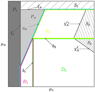
Figure 1. The parameter plane $({\mu }_{{L}},{\mu }_{{R}})$ of the map f for $0<a_{{L}}<1$ and $a_{{R}}>1$. The regions ${{P}}_{{L}}$, ${{P}}_{{M}}$ are related to stable fixed points. The regions S₁, S₂, S₃ are related to diverging orbits. The regions D₁, D₂, and D₀ are associated with asymptotic orbits located in $I_{{L}}\cup I_{{M}}$, $I_{{M}}\cup I_{{R}}$, and $I_{{L}}\cup I_{{M}}\cup I_{{R}}$, respectively.

The function f can have at most three fixed points¹, one in each partition I_s, $s\in \left\{{L},{M},{R}\right\}$. A fixed point ${{O}}_s$, $s\in \left\{{L},{R}\right\}$, given by x_s = μ_s/(1 − a_s) appears/disappears through collision with the border point d_s. The related bifurcation boundary is

$\begin{array}{ll}{\xi }_s=\left\{p:{\mu }_s=(1-a_s)d_s\right\}.& (3)\end{array}$

Notice that the upper index d_s is omitted in the notation ξ_s because it is clear that at ${\xi }_{{L}}$ the collision occurs with $d_{{L}}$ while at ${\xi }_{{R}}$ it occurs with $d_{{R}}$. Below, for shortness, we drop upper indices in notations for BCB boundaries whenever it is clear which border point is involved in the bifurcation (namely, when the first symbol of σ is ${L}$ or ${R}$ the related border point is $d_{{L}}$ or $d_{{R}}$, respectively).

From 0 ⩽ a_s < 1 the stability regions of ${{O}}_{{L}}$ and ${{O}}_{{R}}$ are obtained:

$\begin{array}{l}{{P}}_{{L}}=\{p:{\mu }_{{L}}<\left(1-a_{{L}}\right)d_{{L}},0⩽a_{{L}}<1\},\\ {{P}}_{{R}}=\{p:{\mu }_{{R}}>\left(1-a_{{R}}\right)d_{{R}},0⩽a_{{R}}<1\}.& (4)\end{array}$

The stability region ${{P}}_s$ is separated from the divergence region ${{S}}_s$ by the boundary a_s = 1, where

$\begin{array}{ll}\begin{array}{c}{{S}}_{{L}}=\left\{p:{\mu }_{{L}}<(1-a_{{L}})d_{{L}},{\mu }_{{R}}<(1-a_{{R}})d_{{R}},a_{{L}}>1\right\},\\ {{S}}_{{R}}=\left\{p:{\mu }_{{R}}>(1-a_{{R}})d_{{R}},{\mu }_{{L}}>(1-a_{{L}})d_{{L}},a_{{R}}>1\right\}\end{array}& (5)\end{array}$

(see Figure 1 where ${{P}}_{{L}}$ and ${{S}}_{{R}}$ are shown).

The region

$\begin{array}{l}{{P}}_{{M}}=\{p:{\mu }_{{L}}>\left(1-a_{{L}}\right)d_{{L}},{\mu }_{{L}}+\left(1+a_{{L}}\right)\\ d_{{L}}-\left(1+a_{{R}}\right)d_{{R}}<{\mu }_{{R}}<\left(1-a_{{R}}\right)d_{{R}}\},& (6)\end{array}$

associated with the attracting fixed point ${{O}}_{{M}}$ given by $x_{{M}}={\mu }_{{M}}/(1-a_{{M}})$, is confined by three boundaries. Namely, the BCB boundary ${\xi }_{{L}}$, the BCB boundary ${\xi }_{{R}}$, and the DFB boundary

$\begin{array}{ll}{\eta }_{{M}}=\left\{p:{\mu }_{{R}}={\mu }_{{L}}+(1+a_{{L}})d_{{L}}-(1+a_{{R}})d_{{R}}\right\},& (7)\end{array}$

related to the condition $a_{{M}}=-1$.

The rest of parameter space is occupied by the region

$\begin{array}{l}D=\{p:{\mu }_{{L}}>\left(1-a_{{L}}\right)d_{{L}},{\mu }_{{R}}<\left(1-a_{{R}}\right)d_{{R}},\\ {\mu }_{{R}}<{\mu }_{{L}}+\left(1+a_{{L}}\right)d_{{L}}-\left(1+a_{{R}}\right)d_{{R}}\},& (8)\end{array}$

which is marked by blue line in Figure 1. First, we notice that for certain parameter values asymptotic orbits of f are located only on the two adjacent branches. Namely,

1. If $\ell <d_{{R}}$ then only $I_{{L}}$ and $I_{{M}}$ are relevant for asymptotic dynamics of f. Hence, the surfaces ${\xi }_{{L}}$, ${\eta }_{{M}}$, and b₁ (defined from the condition $\ell =d_{{R}}$) confine the region

$\begin{array}{l}{D}_1=\{p:(1-a_{{L}})d_{{L}}<{\mu }_{{L}}<d_{{R}}-d_{{L}}{a}_{{L}},\\ {\mu }_{{R}}<{\mu }_{{L}}+\left(1+a_{{L}}\right)d_{{L}}-\left(1+a_{{R}}\right)d_{{R}}\}& (9)\end{array}$

(outlined red in Figure 1). The related bifurcation structure—skew tent map (STM for short) structure—is described in Section 3.

2. Similarly, the condition $r>d_{{L}}$ holds in the region

$\begin{array}{l}{D}_2=\{p:d_{{L}}-d_{{R}}{a}_{{R}}<{\mu }_{{R}}<(1-a_{{R}})d_{{R}},\\ {\mu }_{{R}}<{\mu }_{{L}}+\left(1+a_{{L}}\right)d_{{L}}-\left(1+a_{{R}}\right)d_{{R}}\},& (10)\end{array}$

(outlined yellow in Figure 1). This region, also having the STM structure, is confined by ${\xi }_{{R}}$, ${\eta }_{{M}}$, and the boundary b₂ corresponding to the condition $r=d_{{L}}$. For p ∈ D₂ only $I_{{M}}$ and $I_{{R}}$ are relevant for asymptotic dynamics of f (see Section 3).

Finally, the conditions $\ell >d_{{R}}$ and $r<d_{{L}}$ define the region

$\begin{array}{ll}{D}_0=\left\{p:{\mu }_{{R}}<d_{{L}}-d_{{R}}{a}_{{R}},{\mu }_{{L}}>d_{{R}}-d_{{L}}{a}_{{L}}\right\},& (11)\end{array}$

delineated green in Figure 1). For parameter values belonging to D₀, orbits of f are located on either $I_{{L}}$ and $I_{{R}}$, or involve all three partitions. Two basic bifurcation structures observed in the region D₀ are period adding (PA for short) structure and fin structure, described in Section 4.

Figure 2A presents an example of the typical bifurcation structure related to regular dynamics in the $({\mu }_{{L}},{\mu }_{{R}})$ parameter plane of the map f (the colors correspond to periods of cycles as indicated in the color bar). In Figure 2B, on the contrary, colored zones correspond to chaoticity regions related to chaotic attractors with different number of intervals (colors correspond to the number of intervals), while periodicity regions are painted gray.

FIGURE 2

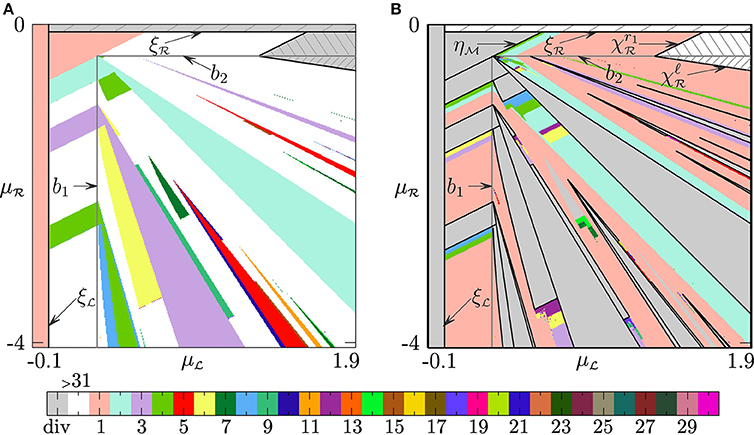
Figure 2. Bifurcation structure of the $({\mu }_{{L}},{\mu }_{{R}})$-parameter plane of f. (A) Regular dynamics: colors correspond to periods of related cycles, while gray hatched areas are associated with diverging orbits. (B) Chaotic dynamics: periodicity regions are shown in gray, while chaoticity regions related to chaotic attractors with different number of intervals are shown with different colors. Parameters: $a_{{L}}=0.5,a_{{R}}=1.3,d_{{L}}=0,d_{{R}}=0.3$.

In the following sections we characterize different bifurcation structures observed in the parameter space of the map (1).

3. Skew Tent Map Structure

Let p ∈ D₁ or p ∈ D₂, then asymptotic dynamics of the map (1) is associated with two adjacent partitions only. In such a case the map f is locally topologically conjugate to the famous skew tent map, which was extensively studied already three decades ago (see e.g., [7–10]). Below we summarize main facts concerning this bifurcation structure, which we refer to as the skew tent map (STM) structure.

Let us consider the skew tent map family g_α,β,μ

$g_{\alpha ,\beta ,\mu }:x\to g_{\alpha ,\beta ,\mu }(x)=\{\begin{array}{l}{g}_{{A}}(x)=\alpha x+\mu ,x⩽0,\hfill \\ g_B(x)=\beta x+\mu ,x>0,\hfill \end{array}(12)$

with αβ < 0. All maps from this family with μ > 0 (μ < 0) are topologically equivalent to g_α,β,1 (g_α,β,−1). Moreover, g_α,β,−1 is topologically equivalent to g_β,α,1. Hence, to describe the STM structure it is enough to fix μ = 1. Non-trivial dynamics in this case is observed for α > 0, β < 0. Below, for shortness, we drop the indices denoting the parameters and refer to the skew tent map simply as g.

Any point x < 0 is associated with the symbol ${A}$, while a point x > 0 corresponds to the symbol ${B}$. The critical point is denoted as c := g(0) and its images as $c_i:=g^i(c)$.

The stability region of the fixed point ${{O}}_{{B}}$ is confined by the DB1 boundary ${\theta }_{{B}}=\left\{(\alpha ,\beta ):\beta =1\right\}$ and the DFB boundary ${\eta }_{{B}}=\left\{(\alpha ,\beta ):\beta =-1\right\}$.

The only possible stable cycles of g are the basic n-cycles ${{O}}_{{B}{{A}}^{n-1}}$, n ⩾ 2. Each periodicity region ${{P}}_{{B}{{A}}^{n-1}}$ is confined by the BCB boundary and the DFB boundary

$\begin{array}{lll}{\xi }_{{A}{B}{{A}}^{n-2}}& =& \left\{(\alpha ,\beta ):\beta =-\frac{1-{\alpha }^{n-1}}{(1-\alpha ){\alpha }^{n-2}}\right\},\\ {\eta }_{{B}{{A}}^{n-1}}& =& \left\{(\alpha ,\beta ):\beta =-\frac{1}{{\alpha }^{n-1}}\right\}& (13)\end{array}$

(see Figure 3 where the boundaries ${\xi }_{{A}{B}{A}}$ and ${\eta }_{{B}{{A}}^2}$ are marked). The BCB boundary ${\xi }_{{A}{B}}$ is particular, because it coincides with the DFB boundary ${\eta }_{{B}}$. For every n ⩾ 3 the boundary ${\xi }_{{A}{B}{{A}}^{n-2}}$ corresponds to the fold BCB leading to the appearance of the basic cycle ${{O}}_{{B}{{A}}^{n-1}}$ and its complementary cycle ${{O}}_{{{B}}^2{{A}}^{n-2}}$ which is necessarily unstable. The boundary ${\eta }_{{B}{{A}}^{n-1}}$, n ⩾ 3, is related to the DFB of the cycle ${{O}}_{{B}{{A}}^{n-1}}$, which leads to the appearance of 2n-cyclic chaotic intervals ${{Q}}_{2n}$. The DFB of the fixed point ${{O}}_{{B}}$ and the 2-cycle ${{O}}_{{B}{A}}$ are particular as described below.

FIGURE 3

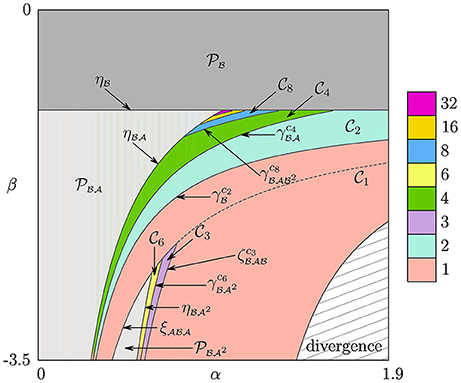
Figure 3. Bifurcation structure of (α, β) parameter plane of the skew tent map.

The chaoticity region ${{C}}_{2n}$, n ⩾ 3, associated with ${{Q}}_{2n}$, is the area restricted between ${\xi }_{{A}{B}{{A}}^{n-2}}$, ${\eta }_{{B}{{A}}^{n-1}}$, and ${\gamma }_{{B}{{A}}^{n-1}}^{c_{2n}}$. The latter one is related to the first homoclinic bifurcation of the cycle ${{O}}_{{B}{{A}}^{n-1}}$. This bifurcation occurs when

$\begin{array}{ll}{c}_{2n}=x_{{B}{{A}}^{n-1}}\text{\hspace{1em}with\hspace{1em}}{c}_{2n}=g_{{B}{{A}}^{n-1}{B}{{A}}^{n-2}{B}}(c).& (14)\end{array}$

The condition (14) holds for

$\begin{array}{ll}{\gamma }_{{B}{{A}}^{n-1}}^{c_{2n}}=\left\{(\alpha ,\beta ):{\alpha }^{2(n-1)}{\beta }^3-\beta +\alpha =0\right\}.& (15)\end{array}$

Crossing the bifurcation boundary ${\gamma }_{{B}{{A}}^{n-1}}^{c_{2n}}$ leads to the transition ${{Q}}_{2n}\Rightarrow {{Q}}_n$, which is also called the merging bifurcation. The existence region for n-cyclic chaotic intervals ${{Q}}_n$ is ${{C}}_n$ confined by ${\xi }_{{A}{B}{{A}}^{n-2}}$, boundary ${\gamma }_{{B}{{A}}^{n-1}}^{c_{2n}}$, and the boundary ${\zeta }_{{B}{{A}}^{n-2}{B}}^{c_n}$ corresponding to the first homoclinic bifurcation of the cycle ${{O}}_{{{B}}^2{{A}}^{n-2}}$. This homoclinic bifurcation occurs when

$\begin{array}{ll}{c}_n=g_{{B}{{A}}^{n-1}}(c)=x_{{B}{{A}}^{n-2}{B}},& (16)\end{array}$

which gives

$\begin{array}{ll}{\zeta }_{{B}{{A}}^{n-2}{B}}^{c_n}=\left\{(\alpha ,\beta ):{\alpha }^{n-1}{\beta }^2+\beta -\alpha =0\right\}.& (17)\end{array}$

Crossing the boundary ${\zeta }_{{B}{{A}}^{n-2}{B}}^{c_n}$ leads to the transition ${{Q}}_n\Rightarrow {Q}$, which is also called the expansion bifurcation. For more detailed description of merging and expansion bifurcations we refer to Avrutin et al. [18]. In Figure 3 the boundaries ${\gamma }_{{B}{{A}}^2}^{c_6}$ and ${\zeta }_{{B}{A}{B}}^{c_3}$ are marked.

Cases n = 1 and n = 2 differ from the others. The DFB of the fixed point ${{O}}_{{B}}$ leads either to an attracting 2-cycle or to 2^m-cyclic chaotic intervals, where m ⩾ 1 depends on particular parameter values. As for the 2-cycle ${{O}}_{{A}{B}}$, when it loses stability due to DFB, there can appear 2^m-cyclic chaotic intervals ${{Q}}_{2^m}$, where m ⩾ 2 depends on α, β. Every region ${{C}}_{2^m}$ is adjacent to ${{C}}_{2^{m-1}}$ from one side and to ${{C}}_{2^{m+1}}$ from the other side. The boundary separating ${{C}}_{2^m}$ and ${{C}}_{2^{m+1}}$ is associated with the first homoclinic bifurcation of the 2^m-cycle whose symbolic sequence is the m-th harmonic of ${B}$. Recall that to obtain the k-harmonic ρ_k of ${B}$ one has to apply concatenation operator iteratively as follows:

$\begin{array}{ll}{\rho }_0:={B},{\rho }_0^{\prime }:={A},{\rho }_k={\rho }_{k-1}{\rho }_{k-1}^{\prime },k⩾1,& (18)\end{array}$

where ${\rho }_{k-1}^{\prime }$ differs from ρ_k−1 only by the last symbol. For example, ${\rho }_1={B}{A}$, ${\rho }_2={B}{A}{B}{B}$, ${\rho }_3={B}{A}{B}{B}{B}{A}{B}{A}$, and so on. Notice that according to the rule (18) it is possible to define harmonics of an arbitrary cycle ${{O}}_{\sigma }$ provided that x_σ is the rightmost point of the cycle. For instance, in the condition (14) for the first homoclinic bifurcation of ${{O}}_{{B}{{A}}^{n-1}}$ the symbolic sequence ${B}{{A}}^{n-1}{B}{{A}}^{n-2}{B}$ is the first harmonic of ${B}{{A}}^{n-1}$.

The condition for the first homoclinic bifurcation of the 2^m-cycle ${{O}}_{{\rho }_m}$ is

$\begin{array}{ll}{g}_{{\rho }_{m+1}}(c)=x_{{\rho }_m},& (19)\end{array}$

that holds for

$\begin{array}{ll}{\gamma }_{{\rho }_m}^{c_{2^{m+1}}}=\left\{(\alpha ,\beta ):{\alpha }^{2{\delta }_m}{\beta }^{2{\delta }_{m+1}}+{\left(\frac{\alpha }{\beta }\right)}^{{(-1)}^{m+1}}-1=0\right\},& (20)\end{array}$

where ${\delta }_m=(2^m-{(-1)}^m)/3$, m ⩾ 1. As mentioned above this bifurcation leads to the transition ${{Q}}_{2^{m+1}}\Rightarrow {{Q}}_{2^m}$, The case m = 0 (i.e., the merging bifurcation ${\gamma }_{{\rho }_0}^{c_2}$) is related to the first homoclinic bifurcation of the fixed point ${{O}}_{{B}}$ leading to the transition ${{Q}}_2\Rightarrow {Q}$. For m → ∞ the curves ${\gamma }_{{\rho }_m}^{c_{2^{m+1}}}$ in the (α, β)-plane crowd the point (α, β) = (1, −1) (see Figure 3).

The region related to diverging orbits (hatched in Figure 3) is confined by the boundary related to the first homoclinic bifurcation of the fixed point ${{O}}_{{A}}$, which occurs when $c_1=g_{{B}}(c)=x_{{A}}$:

$\begin{array}{ll}{\chi }_{{A}}^{c_1}=\left\{(\alpha ,\beta ):\beta =\frac{\alpha }{1-\alpha }\right\}.& (21)\end{array}$

At this bifurcation the absorbing interval J = [c₁, c] collides with a boundary of its basin of attraction (given by ${{O}}_{{A}}$ and its preimage) and for $\beta <\frac{\alpha }{1-\alpha }$ the interval J is no longer absorbing causing a typical orbit to diverge. Such bifurcation is also called a final bifurcation.

For p ∈ D₁ or p ∈ D₂ the original map f is locally topologically conjugate to g with $\beta =a_{{M}}$, $\alpha =a_{{L}}$ or $\alpha =a_{{R}}$, respectively, and μ = 1 in the neighborhood of $d_{{L}}$ or $d_{{R}}$, respectively. Thus, to get the boundaries of STM-regions in the parameter space of f it is enough to substitute ${L}$ or ${R}$, respectively, instead of ${A}$ and ${M}$ instead of ${B}$. In Figure 4 the STM-regions in the $({\mu }_{{L}},{\mu }_{{R}})$ parameter plane associated with attracting cycles are colored with moderate gray, while for chaoticity regions only their boundaries are shown (blue lines). The hatched region in D₂ is related to diverging orbits.

FIGURE 4

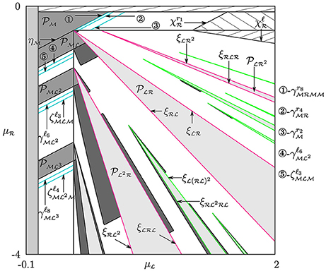
Figure 4. Bifurcation structure of the $({\mu }_{{L}},{\mu }_{{R}})$-parameter plane of map f: periodicity regions of the STM structure, as well as the PA and the fin structures are shown moderate gray, light-gray, and dark-gray, respectively. For chaoticity regions of the STM structure their boundaries are shown with blue lines. For PA regions of the first complexity level their boundaries are plotted red, while green color corresponds to the second complexity level. The parameters are as in Figure 2.

4. Bifurcation Structures Involving Both Border Points: Regular Dynamics

Let us briefly recall how other two periodicity structures are formed in the parameter space of f for p ∈ D₀.

4.1. Period Adding Structure

Consider a cycle ${{O}}_{\sigma }$ of the map f with $a_{{L}}>0$, $a_{{R}}>0$ such that all its points belong only to $I_{{L}}\cup I_{{R}}$. Consequently, σ consists only of the symbols ${L}$ and ${R}$. Then the related periodicity region ${{P}}_{\sigma }$ is a part of the so-called period adding structure (PA structure). Such structures are also known as Arnold tongues or mode-locking tongues and often appear in the parameter space of a certain class of circle maps, 1D discontinuous maps, two- and higher-dimensional maps near a Neimark-Sacker bifurcation boundary, etc. (see, for example [3, 24–27]). We recall that the regions belonging to PA structure are located in the parameter space according to a specific order based on Farey summation rule. Namely, consider two cycles ${{O}}_{{\sigma }_1}$ of period n₁ and ${{O}}_{{\sigma }_2}$ of period n₂ with σ_i containing m_i symbols ${L}$. Suppose also that the fractions m₁/n₁ and m₂/n₂, called also rotation numbers, are Farey neighbors, that is, |m₁n₂ − m₂n₁| = 1. Then in the parameter space between the two regions related to ${{O}}_{{\sigma }_1}$ and ${{O}}_{{\sigma }_2}$ there is a region related to a cycle ${{O}}_{{\sigma }_3}$ of periodicity n₁ + n₂ with σ₃ having m₁ + m₂ symbols ${L}$, and thus, the rotation number of ${{O}}_{{\sigma }_3}$ is (m₁ + m₂)/(n₁ + n₂). Notice that the cycles ${{O}}_{{\sigma }_i}$, i = 1, 2, 3, are not necessarily attracting.

In Figure 4 the regions composing the PA structure are shown light-gray.

If $0<a_{{L}},a_{{R}}<1$ then any PA-cycle is globally attracting inside the region of its existence. Indeed, in this case for p ∈ D₀ there always exists an invariant absorbing interval J = [r, ℓ], and hence, there are no divergent orbits. Moreover, we consider an arbitrary PA-cycle ${{O}}_{\sigma }$ and immediately get that its multiplier is ${\nu }_{\sigma }=a_{{L}}^m{a}_{{R}}^{n-m}\in (0,1)$, where m is the number of ${L}$'s in σ.

However, if one of the slopes is greater than one, while the other is between zero and one, the inequality ν_σ < 1 is satisfied only if $n<m(1-{log}_{a_{{R}}}{a}_{{L}})$, so that not all PA-cycles are attracting. There can also be divergent orbits since there is an unstable fixed point on the branch whose slope is greater than one. Furthermore, the interval J is no longer absorbing after the final bifurcation corresponding to the first homoclinic bifurcation of this unstable fixed point. The related bifurcation boundary confines the region in the parameter space in which a typical orbit diverges. For instance, for $0<a_{{L}}<1$, $a_{{R}}>1$ (as in Figure 4) the final bifurcation ${\chi }_{{R}}^{\ell }$ occurs when $x_{{R}}=\ell$, and thus, for any $(1-a_{{R}})(a_{{L}}{d}_{{L}}+{\mu }_{{L}})<{\mu }_{{R}}<d_{{L}}-a_{{R}}{d}_{{R}}$ all orbits go to infinity.

To simplify calculation of analytic expressions for PA-region boundaries we use the so-called map replacement technique [28]. At first we group symbolic sequences of PA-cycles into infinite number of families complying with their complexity level (as in [3]). For example, two families related to basic cycles form the first complexity level:

$\begin{array}{ll}{\Sigma }_{1,1}={\left\{{L}{{R}}^{n_1}\right\}}_{n_1=1}^{\infty },{\Sigma }_{2,1}={\left\{{R}{{L}}^{n_1}\right\}}_{n_1=1}^{\infty }.& (22)\end{array}$

Notice that both families contain the common sequence ${L}{R}\equiv {R}{L}$.

To construct the rest of symbolic sequence families we introduce the following symbolic replacements:

${\kappa }_m^{{L}}:=\{\begin{array}{l}{L}\to {L}{{R}}^m\hfill \\ {R}\to {R}{L}{{R}}^m\hfill \end{array},{\kappa }_m^{{R}}:=\{\begin{array}{l}{L}\to {L}{R}{{L}}^m\hfill \\ {R}\to {R}{{L}}^m\hfill \end{array}.(23)$

Application of a symbolic replacement ${\kappa }_m^{{L}}$ to a symbolic sequence σ means that each symbol ${L}$ in σ is replaced by ${L}{{R}}^m$ and each symbol ${R}$ by ${R}{L}{{R}}^m$. Similarly, application of ${\kappa }_m^{{R}}$ means replacing all ${L}$'s by ${L}{R}{{L}}^m$ and all ${R}$'s by ${R}{{L}}^m$.

Symbolic sequences of higher complexity levels are obtained by iterative application of ${\kappa }_m^{{L}}$ and ${\kappa }_m^{{R}}$. More precisely, applying ${\kappa }_{n_2}^{{L}}$ and ${\kappa }_{n_2}^{{R}}$ to Σ_1,1 we get the families

$\begin{array}{l}{\Sigma }_{1,2}={\left\{{L}{{R}}^{n_2}{({R}{L}{{R}}^{n_2})}^{n_1}\right\}}_{n_1,n_2=1}^{\infty },\\ {\Sigma }_{2,2}={\left\{{L}{R}{{L}}^{n_2}{({R}{{L}}^{n_2})}^{n_1}\right\}}_{n_1,n_2=1}^{\infty }.& (24)\end{array}$

And then applying ${\kappa }_{n_2}^{{L}}$ and ${\kappa }_{n_2}^{{R}}$ to Σ_2,1 we obtain

$\begin{array}{l}{\Sigma }_{3,2}={\left\{{R}{L}{{R}}^{n_2}{({L}{{R}}^{n_2})}^{n_1}\right\}}_{n_1,n_2=1}^{\infty },\\ {\Sigma }_{4,2}={\left\{{R}{{L}}^{n_2}{({L}{R}{{L}}^{n_2})}^{n_1}\right\}}_{n_1,n_2=1}^{\infty }.& (25)\end{array}$

The four families Σ_i,2, $i=\overline{1,4}$, compose the second complexity level. Notice that the families Σ_1,2 and Σ_3,2 contain the common sequence ${L}{R}{R}{L}{R}\equiv {R}{L}{R}{L}{R}$ with n₁ = n₂ = 1, while Σ_2,2 and Σ_4,2 share the sequence ${L}{R}{L}{R}{L}\equiv {R}{L}{L}{R}{L}$ with n₁ = n₂ = 1.

In short the applied procedure can be written as

$\begin{array}{l}{\Sigma }_{1,2}={\kappa }_{n_2}^{{L}}({\Sigma }_{1,1}),{\Sigma }_{2,2}={\kappa }_{n_2}^{{R}}({\Sigma }_{1,1}),\\ {\Sigma }_{3,2}={\kappa }_{n_2}^{{L}}({\Sigma }_{2,1}),{\Sigma }_{4,2}={\kappa }_{n_2}^{{R}}({\Sigma }_{2,1}).& (26)\end{array}$

Further, applying the replacements (23) with m = n₃ to four families of the second complexity level, we obtain 2³ families Σ_j,3, $j=\overline{1,2^3}$, of the third complexity level, and so on. In this way all symbolic sequences of PA-cycles are obtained.

Now let us identify the PA-regions in the parameter space of the map f. Each such region has two boundaries corresponding to BCBs of the related cycle. For the basic cycles ${{O}}_{{L}{{R}}^{n_1}}$, n₁ ⩾ 1, these boundaries are obtained directly from the relevant BCB conditions giving

$\begin{array}{ll}\begin{array}{l}{\xi }_{{L}{{R}}^{n_1}}=\left\{p\in D_0:{\mu }_{{L}}={\Phi }_{1,1}(a_{{L}},a_{{R}},{\mu }_{{R}},d_{{L}},n_1)\right\},\\ {\xi }_{{R}{L}{{R}}^{n_1-1}}=\left\{p\in D_0:{\mu }_{{L}}={\text{Ψ}}_{1,1}(a_{{L}},a_{{R}},{\mu }_{{R}},d_{{R}},n_1)\right\},\end{array}& (27)\end{array}$

where

$\begin{array}{ll}{\Phi }_{1,1}(a_{{L}},a_{{R}},{\mu }_{{R}},d,n_1)=-\psi (a_{{R}},n_1){\mu }_{{R}}+\phi (a_{{R}},a_{{L}},n_1)d,& (28)\end{array}$

$\begin{array}{l}{\text{Ψ}}_{1,1}(a_{{L}},a_{{R}},{\mu }_{{R}},d,n_1)=-(a_{{L}}+\psi (a_{{R}},n_1-1)){\mu }_{{R}}\\ +a_{{R}}\phi (a_{{R}},a_{{L}},n_1)d& (29)\end{array}$

with

$\begin{array}{ll}\phi (a,b,n)=\frac{1-a^{n}b}{a^n},\psi (a,n)=\frac{1-a^n}{(1-a)a^n}.& (30)\end{array}$

For ${{O}}_{{R}{{L}}^{n_1}}$, n ⩾ 1, their boundaries are obtained from (27) by interchanging ${L}$ and ${R}$. So that, the basic PA-regions are defined as

$\begin{array}{l}{{P}}_{{L}{{R}}^{n_1}}=\{p\in D_0:{\Psi }_{1,1}(a_{{L}},a_{{R}},{\mu }_{{R}},d_{{R}},n_1)<{\mu }_{{L}}\\ <{\Phi }_{1,1}(a_{{L}},a_{{R}},{\mu }_{{R}},d_{{L}},n_1)\},& (31)\end{array}$

$\begin{array}{l}{{P}}_{{R}{{L}}^{n_1}}=\{p\in D_0:{\Psi }_{1,1}(a_{{R}},a_{{L}},{\mu }_{{L}},d_{{L}},n_1)>{\mu }_{{R}}\\ >{\Phi }_{1,1}(a_{{R}},a_{{L}},{\mu }_{{L}},d_{{R}},n_1)\}.& (32)\end{array}$

Further, using the map replacement technique we obtain periodicity regions associated with cycles whose symbolic sequences belong to the families Σ_1,2 and Σ_2,2, given in (24). The trick is as follows. Any symbolic sequence τ ∈ Σ_1,2 can be written as $\tau ={\kappa }_{n_2}^{{L}}(\sigma )$ with certain n₂ ⩾ 1 and σ ∈ Σ_1,1 with particular n₁ ⩾ 1. Then to get the BCBs ${\xi }_{\tau }^{d_{{L}}}$ and ${\xi }_{\tau }^{d_{{R}}}$ we take the expressions (27) for ${\xi }_{{L}{{R}}^{n_1}}$ and ${\xi }_{{R}{L}{{R}}^{n_1-1}}$ and substitute the parameters $a_{{L}}$, ${\mu }_{{L}}$, $a_{{R}}$, ${\mu }_{{R}}$ by $a_{{L}{{R}}^{n_2}}$, ${\mu }_{{L}{{R}}^{n_2}}$, $a_{{R}{L}{{R}}^{n_2-1}}$, ${\mu }_{{R}{L}{{R}}^{n_2-1}}$:

$\begin{array}{l}{\xi }_{{\kappa }_{n_2}^{{L}}({L}{{R}}^{n_1})}=\{p\in D_0:{\mu }_{{L}{{R}}^{n_2}}={\Phi }_{1,1}(a_{{L}{{R}}^{n_2}},a_{{R}{L}{{R}}^{n_2-1}},\\ {\mu }_{{R}{L}{{R}}^{n_2-1}},d_{{L}},n_1)\},\\ {\xi }_{{\kappa }_{n_2}^{{L}}({R}{L}{{R}}^{n_1-1})}=\{p\in D_0:{\mu }_{{L}{{R}}^{n_2}}={\Psi }_{1,1}(a_{{L}{{R}}^{n_2}},a_{{R}{L}{{R}}^{n_2-1}},\\ {\mu }_{{R}{L}{{R}}^{n_2-1}},d_{{R}},n_1)\}.& (33)\end{array}$

Recall that $a_{{L}{{R}}^{n_2}}$, ${\mu }_{{L}{{R}}^{n_2}}$ and $a_{{R}{L}{{R}}^{n_2-1}}$, ${\mu }_{{R}{L}{{R}}^{n_2-1}}$ denote, respectively, the coefficients of the following composite (auxiliary) functions

$\begin{array}{l}{f}_{{L}{{R}}^{n_2}}=f_{{L}}○{\displaystyle \underset{n_2}{{\displaystyle \underbrace{f_{{R}}○\cdots ○f_{{R}}}}}},f_{{R}{L}{{R}}^{n_2-1}}=f_{{R}}○f_{{L}}○{\displaystyle \underset{n_2-1}{{\displaystyle \underbrace{f_{{R}}○\cdots ○f_{{R}}}}}}.\end{array}$

Schematically, we summarize the applied procedure as follows:

$\begin{array}{ll}\begin{array}{c}{\xi }_{{L}{{R}}^{n_1}}{\displaystyle \underset{{L}\to {L}{{R}}^{n_2}{R}\to {R}{L}{{R}}^{n_2-1}}{\overset{}{\to }}}{\xi }_{{\kappa }_{n_2}^{{L}}({L}{{R}}^{n_1})},\\ {\xi }_{{R}{L}{{R}}^{n_1-1}}{\displaystyle \underset{{L}\to {L}{{R}}^{n_2}{R}\to {R}{L}{{R}}^{n_2-1}}{\overset{}{\to }}}{\xi }_{{\kappa }_{n_2}^{{L}}({R}{L}{{R}}^{n_1-1})}.\end{array}& (34)\end{array}$

Clearly, the coefficients $a_{{L}{{R}}^{n_2}}$, ${\mu }_{{L}{{R}}^{n_2}}$, $a_{{R}{L}{{R}}^{n_2-1}}$, ${\mu }_{{R}{L}{{R}}^{n_2-1}}$ depend on $a_{{L}}$, ${\mu }_{{L}}$, $a_{{R}}$, ${\mu }_{{R}}$, and hence, the equalities in (33) can be solved with respect to ${\mu }_{{L}}$, implying the PA-region related to ${{O}}_{{\kappa }_{n_2}^{{L}}({L}{{R}}^{n_1})}$ to be

$\begin{array}{l}{{P}}_{{\kappa }_{n_2}^{{L}}({L}{{R}}^{n_1})}=\{p\in D_0:{\Psi }_{1,2}(a_{{L}},a_{{R}},{\mu }_{{R}},d_{{R}},n_1,n_2)\\ <{\mu }_{{L}}<{\Phi }_{1,2}(a_{{L}},a_{{R}},{\mu }_{{R}},d_{{L}},n_1,n_2)\}& (35)\end{array}$

where Ψ_1,2, Φ_1,2 are certain functions (see [16] where expressions for Ψ_1,2, Φ_1,2 are given in explicit form).

Similarly, any symbolic sequence τ ∈ Σ_2,2 can be written as $\tau ={\kappa }_{n_2}^{{R}}(\sigma )$ with n₂ ⩾ 1 and σ ∈ Σ_1,1. To get the expressions for the boundaries of ${{P}}_{\tau }$ we perform analogous trick replacing in (27) the parameters $a_{{L}}$, ${\mu }_{{L}}$, $a_{{R}}$, ${\mu }_{{R}}$ with the coefficients $a_{{L}{R}{{L}}^{n_2-1}}$, ${\mu }_{{L}{R}{{L}}^{n_2-1}}$, $a_{{R}{{L}}^{n_2}}$, ${\mu }_{{R}{{L}}^{n_2}}$ of the related (auxiliary) composite functions. The resulting new equalities can be resolved with respect to ${\mu }_{{L}}$, and the related PA-region is

$\begin{array}{l}{{P}}_{{\kappa }_{n_2}^{{R}}({L}{{R}}^{n_1})}=\{p\in D_0:{\Psi }_{2,2}(a_{{L}},a_{{R}},{\mu }_{{R}},d_{{R}},n_1,n_2)<{\mu }_{{L}}\\ <{\Phi }_{2,2}(a_{{L}},a_{{R}},{\mu }_{{R}},d_{{L}},n_1,n_2)\}.(36)\end{array}$

with certain Ψ_2,2, Φ_2,2.

As for the cycles whose symbolic sequences belong to the families Σ_3,2 and Σ_4,2 (25), boundaries of the related periodicity regions are obtained by interchanging the indices ${L}$ and ${R}$ and changing the inequality signs to the opposite ones in (36) and (35), respectively.

Similarly, having expressions for the boundaries of periodicity regions of the (k − 1)-th complexity level and using this replacement technique, we can compute the related expressions for periodicity regions of the k-th complexity level (for more detail see [16]).

In Figure 4 for the regions of the first complexity level their boundaries are colored red, while for those of the second complexity level they are green.

4.2. Fin Structure

In Figure 2 or in Figure 4 one can notice that some PA-regions have other (smaller) periodicity regions attached to them, which resemble to certain extent fish fins. Every such fin-like region is associated with a stable kn-cycle, where n is the period of the related PA-cycle and k ⩾ 1. To explain briefly how these regions appear, let us consider the n-th iterate of f.

For the map fⁿ every point of the PA-cycle, say ${{O}}_{\sigma }$, of the period n is a fixed point. Suppose that the parameter point $p\in {{P}}_{\sigma }$ moves outside the region crossing transversally, for instance, the boundary ${\xi }_{\sigma }^{d_{{L}}}$ (see Figure 5). Near the BCB the map fⁿ is locally topologically conjugate in the neighborhood of $d_{{L}}$ to a skew tent map g_α,β,μ (12) with $\alpha =a_{{L}}^l{a}_{{R}}^{n-l}$, $\beta =a_{{L}}^{l-1}{a}_{{M}}{a}_{{R}}^{n-l}$ (l is the number of symbols ${L}$ in σ) and μ < 0 before, μ = 0 at, and μ > 0 after the bifurcation. In other words, the skew tent map is used as the BCB normal form, and the result of such a bifurcation is completely defined by the values of α and β (see, e.g., [5, 10, 11]). In particular, for certain combination of $a_{{L}}$, $a_{{M}}$ and $a_{{R}}$, a stable k-cycle for fⁿ appears after the BCB. In terms of the original map f, after the BCB of a stable n-cycle ${{O}}_{\sigma }$ there occurs a stable kn-cycle, say, ${{O}}_{\tau }$. Crossing the boundary ${\xi }_{\sigma }^{d_{{R}}}$ is treated likewise with the only difference that $\beta =a_{{L}}^l{a}_{{M}}{a}_{{R}}^{n-l-1}$ (for details see [16]).

FIGURE 5

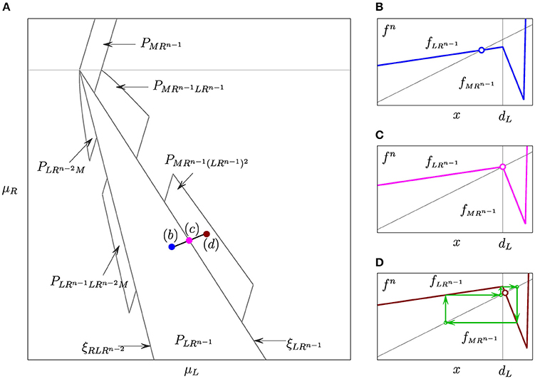
Figure 5. (A) The left and the right 1 · n-, 2 · n-, and 3 · n-fins of the PA-region ${{P}}_{{L}{{R}}^{n-1}}$ shown schematically in the $({\mu }_{{L}},{\mu }_{{R}})$-parameter plane. (B–D) Plots of fⁿ at the corresponding parameter points marked in (A).

We refer to ${{O}}_{\tau }$/${{P}}_{\tau }$ as the k · n-fin cycle/region, and to ${{O}}_{\sigma }$/${{P}}_{\sigma }$ as the trunk cycle/region. For clarity sake, the region ${{P}}_{\tau }$ is called the left/right k · n-fin if it is attached to the boundary of ${{P}}_{\sigma }$ that is related to collision of ${{O}}_{\sigma }$ with the left/right border point $d_{{L}}$/$d_{{R}}$. Furthermore, the complexity level of the trunk region defines the complexity level of its fins.

Let us consider ${{P}}_{{L}{{R}}^{n-1}}$, n ⩾ 2, of the first complexity level. Its left k · n-fin regions, k ⩾ 1, correspond to cycles whose symbolic sequences are

$\begin{array}{ll}{\sigma }_{kn}^{{L}}:={({L}{{R}}^{n-1})}^{k-1}{M}{{R}}^{n-1},& (37)\end{array}$

while symbolic sequences of the cycles associated with right k · n-fin regions are

$\begin{array}{ll}{\sigma }_{kn}^{{R}}:={({R}{L}{{R}}^{n-2})}^{k-1}{M}{L}{{R}}^{n-2}.& (38)\end{array}$

As for the trunk region ${{P}}_{{R}{{L}}^{n-1}}$ its k · n-fins correspond to cycles whose symbolic sequences are obtained from (37) and (38) by interchanging symbols ${L}$ and ${R}$. Whether a trunk region has fins on both sides or none of them is present depends on the parameters.

Every fin region ${{P}}_{{\sigma }_{kn}^s}$, $s\in \left\{{L},{R}\right\}$, k ⩾ 2, obviously has a common BCB boundary with the related trunk region. At most ${{P}}_{{\sigma }_{kn}^s}$ has three more bifurcation boundaries that correspond to two other BCB's and the DFB of the associated cycle. Analytic expressions for the BCB boundaries are obtained by using the skew tent map as border collision normal form. The DFB boundary is given by condition $a_{{L}}^l{a}_{{M}}{a}_{{R}}^{kn-l-1}=-1$, where l is the number of symbols ${L}$ in ${\sigma }_{kn}^s$. For left fins ${{P}}_{{\sigma }_{kn}^{{L}}}$ the expressions are (see [16])

$\begin{array}{lll}{\xi }_{{L}{{R}}^{n-1}}=& \left\{p\in D_0:{\mu }_{{L}}={\Phi }_{1,1}(a_{{L}},a_{{R}},{\mu }_{{R}},d_{{L}},n-1)\right\},& (39)\end{array}$

$\begin{array}{lll}{\eta }_{{\sigma }_{kn}^{{L}}}=& \left\{p\in D_0:a_{{M}}{a}_{{R}}^{k(n-1)}{a}_{{L}}^{k-1}=-1\right\},& (40)\end{array}$

$\begin{array}{lll}{\xi }_{{\sigma }_{kn}^{{L}}}^{d_{{L}}}=& \left\{p\in D_0:a_{{M}}{a}_{{R}}^{n-1}=\frac{a_{{L}}{a}_{{R}}^{n-1}({(a_{{L}}{a}_{{R}}^{n-1})}^{-k+1}-1)}{a_{{L}}{a}_{{R}}^{n-1}-1}\right\}& (41)\end{array}$

$\begin{array}{l}{\xi }_{{\sigma }_{kn}^{{L}}}^{d_{{R}}}=\{p\in D_0:a_{{R}}^{n-1}{a}_{{M}}\frac{{(a_{{R}}^{n-1}{a}_{{L}})}^{k-1}-1}{a_{{R}}^{n-1}{a}_{{L}}-1}\left(\left(a_{{R}}^{n-2}{a}_{{L}}+\frac{a_{{R}}^{n-2}-1}{a_{{R}}-1}\right){\mu }_{{R}}+a_{{R}}^{n-2}{\mu }_{{L}}\right)+\\ a_{{R}}^{(n-1)k}{a}_{{M}}{a}_{{L}}^{(k-1)}{d}_{{R}}+\left(a_{{R}}^{n-2}{a}_{{M}}+\frac{a_{{R}}^{n-2}-1}{a_{{R}}-1}\right){\mu }_{{R}}+a_{{R}}^{n-2}{\mu }_{{M}}=d_{{R}}\},& (42)\end{array}$

where Φ_1,1 is introduced in (28). Notice that the symbolic sequence of the 1 · n-fin cycle is ${\sigma }_n^{{L}}\equiv {M}{{R}}^{n-1}$, and hence, the related periodicity region is confined by only three boundaries: ${\xi }_{{L}{{R}}^{n-1}}$ (39), ${\eta }_{{M}{{R}}^{n-1}}$ (40), and ${\xi }_{{R}{M}{{R}}^{n-2}}$ (42).

Similarly, the bifurcation boundaries confining the right k · n-fin ${{P}}_{{\sigma }_{kn}^{{R}}}$, contiguous to ${{P}}_{{L}{{R}}^{n-1}}$, are

$\begin{array}{lll}{\xi }_{{R}{L}{{R}}^{n-2}}=& \left\{p\in D_0:{\mu }_{{L}}={\text{Ψ}}_{1,1}(a_{{L}},a_{{R}},{\mu }_{{R}},d_{{R}},n-1)\right\}& (43)\end{array}$

$\begin{array}{lll}{\eta }_{{\sigma }_{kn}^{{R}}}=& \left\{p\in D_0:a_{{M}}{a}_{{R}}^{k(n-1)-1}{a}_{{L}}^k=-1\right\},& (44)\end{array}$

$\begin{array}{lll}{\xi }_{{\sigma }_{kn}^{{R}}}^{d_{{R}}}=& \left\{p\in D_0:a_{{L}}{a}_{{M}}{a}_{{R}}^{n-2}=\frac{a_{{L}}{a}_{{R}}^{n-1}({(a_{{L}}{a}_{{R}}^{n-1})}^{-k+1}-1)}{a_{{L}}{a}_{{R}}^{n-1}-1}\right\},& (45)\end{array}$

$\begin{array}{l}{\xi }_{{\sigma }_{kn}^{{R}}}^{d_{{L}}}=\{p\in D_0:a_{{R}}^{n-2}{a}_{{M}}{a}_{{L}}\frac{{(a_{{R}}^{n-1}{a}_{{L}})}^{k-1}-1}{a_{{R}}^{n-1}{a}_{{L}}-1}\left(\frac{a_{{R}}^{n-1}-1}{a_{{R}}-1}{\mu }_{{R}}+a_{{R}}^{n-1}{\mu }_{{L}}\right)+\\ a_{{R}}^{(n-1)k-1}{a}_{{M}}{a}_{{L}}^k{d}_{{L}}+a_{{M}}\frac{a_{{R}}^{n-2}-1}{a_{{R}}-1}{\mu }_{{R}}+a_{{M}}{a}_{{R}}^{n-2}{\mu }_{{L}}+{\mu }_{{M}}=d_{{L}}\},& (46)\end{array}$

where Ψ_1,1 is given in (29). Again the symbolic sequence of the 1 · n-fin cycle is ${\sigma }_n^{{R}}\equiv {M}{L}{{R}}^{n-2}$, and consequently, the periodicity region ${{P}}_{{\sigma }_n^{{R}}}$ is confined by ${\xi }_{{L}{{R}}^{n-1}}$ (39), ${\eta }_{{M}{{R}}^{n-1}}$ (40), and ${\xi }_{{R}{M}{{R}}^{n-2}}$ (42).

In Figure 5 the region ${{P}}_{{L}{{R}}^{n-1}}$ and its fins are shown schematically.

The boundaries of fins contiguous to trunk regions ${{P}}_{{R}{{L}}^{n-1}}$ can be obtained by interchanging the indices ${L}$ and ${R}$ in (39–45). The expressions for the boundaries of fin regions attached to trunk regions of higher complexity levels can be obtained using the map replacement technique mentioned in Section 4.1 (see [16] for details).

5. Expansion of the Absorbing Interval from Two Adjacent Branches Over the Third One

The present section describes the phenomena that occur when the parameter point p crosses the boundary b₁/b₂ entering D₀. As mentioned above, for p ∈ D₁/D₂ the invariant absorbing interval J (if it exists) involves only one border point $d_{{L}}$/$d_{{R}}$ and is located in two partitions only. At the boundary b₁/b₂ the interval J collides with the second border point and expands into the third partition. This implies modification of bifurcation boundaries confining periodicity and chaoticity regions.

5.1. Prolongation of the Skew Tent Map Structure

Recall that for p ∈ D₁ asymptotic orbits of the map f are located in $I_{{L}}\cup I_{{M}}$ only. If additionally either $0⩽a_{{L}}⩽1$, or $a_{{L}}>1$ and $f_{{M}}(\ell )>x_{{L}}$, then there exists invariant absorbing interval $J=\left[f_{{M}}(d_{{L}}),d_{{L}}\right]\subset I_{{L}}\cup I_{{M}}$. Consequently, all bifurcation boundaries in D₁ engage only the left border point $d_{{L}}$ and the critical point ℓ (including its images). Similarly, for p ∈ D₂ the bifurcation conditions are related to the right border point $d_{{R}}$ and the critical point r only. Conversely, for p ∈ D₀ the absorbing interval J (if existent) extends over all three partitions. Hence, a bifurcation may be associated with any border or critical point.

Let us consider first chaoticity regions ${{C}}_{2n}$, ${{C}}_n$ existing after the DFB ${\eta }_{{M}{{L}}^{n-1}}$ of the attracting cycle ${{O}}_{{M}{{L}}^{n-1}}$, n ⩾ 3 (generic case). We describe how their boundaries change when the parameter point p enters D₀ crossing the border b₁ (see, for instance, the regions ${{C}}_6$ and ${{C}}_3$ shown Figure 6A). As described in Section 3, for p ∈ D₁ the DFB of ${{O}}_{{M}{{L}}^{n-1}}$ leads to appearance of 2n-cyclic chaotic intervals ${{Q}}_{2n}$, and thus, the corresponding region ${{C}}_{2n}$ is confined by ${\eta }_{{M}{{L}}^{n-1}}$ and ${\gamma }_{{M}{{L}}^{n-1}}^{{\ell }_{2n}}$. However, the part of ${{C}}_{2n}$ located in D₀ is confined by the other two boundaries. The first one is the fold BCB boundary ${\xi }_{{L}{R}{{L}}^{n-1}{M}{{L}}^{n-2}}$, associated with the collision of the fin cycle ${{O}}_{{R}{{L}}^{n-1}{M}{{L}}^{n-1}}$ with $d_{{L}}$. The second boundary is an extension of ${\gamma }_{{M}{{L}}^{n-1}}^{{\ell }_{2n}}$ to D₀, which we refer to as its D₀-prolongation. This boundary is associated as well with a homoclinic bifurcation of ${{O}}_{{M}{{L}}^{n-1}}$, but its condition differs from the one for ${\gamma }_{{M}{{L}}^{n-1}}^{{\ell }_{2n}}$, as we show below.

FIGURE 6

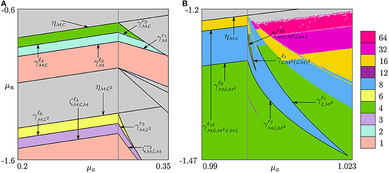
Figure 6. Bifurcation structures associated with D₀-prolongations of the boundaries of the chaoticity regions belonging to the STM structure in D₁. Parameters: (A) $a_{{L}}=0.5$, $a_{{R}}=1.3$, $d_{{L}}=0$, $d_{{R}}=0.3$. (B) $a_{{L}}=0.9$, $a_{{R}}=1.1$, $d_{{L}}=0$, $d_{{R}}=1$.

Figure 7A is a schematic representation of 2n-cyclic chaotic intervals ${{Q}}_{2n}={\left\{J_i\right\}}_{i=0}^{2n-1}$ for $p\in {{C}}_{2n}\subset D_1$. It can be shown that the intervals J_i, $i=\overline{0,2n-2}$, are bounded by ℓ_i+1 and ℓ_i+2n+1 and the interval J_{2n − 1} by ℓ_2n and ℓ. Hence, for p ∈ D₁ the homoclinic bifurcation corresponding to the merging ${{Q}}_{2n}\Rightarrow {{Q}}_n$ can be defined by the following condition:

$\begin{array}{ll}{f}^{2n}(\ell )\equiv f_{{M}{{L}}^{n-1}{M}{{L}}^{n-2}{M}}(\ell )=x_{{M}{{L}}^{n-1}}& (47)\end{array}$

(cf. (14)). For p ∈ b₁, the condition $\ell =d_{{R}}$ holds, and hence ℓ₁ = r, ℓ_i+1 = r_i, i ⩾ 1. Therefore, the intervals J_i, $i=\overline{0,2n-2}$, constituting ${{Q}}_{2n}$ are bounded by ℓ_i+1 = r_i and ℓ_i+2n+1 = r_i+2n, while the interval J_{2n − 1} is given by $\left[r_{2n-1},d_{{R}}\right]$. Hence, the condition (47) becomes

$\begin{array}{l}{f}^{2n}(\ell )\equiv f_{{M}{{L}}^{n-1}{M}{{L}}^{n-2}{M}}(d_{{R}})\equiv f_{{{L}}^{n-1}{M}{{L}}^{n-2}{M}}(r)\\ \equiv f^{2n-1}(r)=x_{{M}{{L}}^{n-1}}.& (48)\end{array}$

FIGURE 7

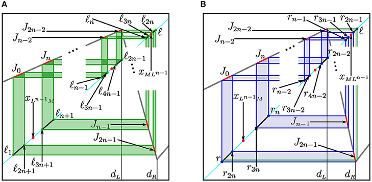
Figure 7. Schematic representation of function f and 2n-cyclic chaotic intervals ${{Q}}_{2n}$ before the merging bifurcation of ${{Q}}_{2n}$ for (A) p ∈ D₁; (B) p ∈ D₀.

As soon as the point p enters the region D₀ by crossing b₁, the absorbing interval J spreads over all three partitions $I_{{L}}$, $I_{{M}}$, and $I_{{R}}$. For ${{Q}}_{2n}$ it means that $J_{2n-1}=\left[r_{2n-1},\ell \right]\subset I_{{M}}\cup I_{{R}}$ with $d_{{R}}\in J_{2n-1}$ (see Figure 7B). By definition f(J_{2n − 1}) = J₀. If p is close to b₁, the value of ℓ is greater than the value of $d_{{R}}$, but it is still close to $d_{{R}}$, and thus,

$\begin{array}{l}f(d_{{R}})<f(\ell )<f(r_{2n-1})\iff r<{\ell }_1<r_{2n}.\end{array}$

It entails that $J_0=\left[f(d_{{R}}),f(r_{2n-1})\right]=\left[r,r_{2n}\right]$, while ℓ₁ ∈ J₀. As a result, only the right boundary of J_{2n − 1} is given by ℓ, and its left boundary, as well as the boundaries of the intervals J_i, $i=\overline{0,2n-2}$, are given by the images of r (of the same rank as for p ∈ b₁). Thus, for p ∈ D₀ the condition for the homoclinic bifurcation leading to the transition ${{Q}}_{2n}\Rightarrow {{Q}}_n$ coincides with (48). In such a way the D₀-prolongation of ${\gamma }_{{M}{{L}}^{n-1}}^{{\ell }_{2n}}$ is the merging bifurcation boundary

$\begin{array}{ll}{\gamma }_{{M}{{L}}^{n-1}}^{r_{2n-1}}=\left\{p\in D_0:f_{{{L}}^{n-1}{M}{{L}}^{n-2}{M}}(r)=x_{{M}{{L}}^{n-1}}\right\}.& (49)\end{array}$

Similarly, we deduce that the chaoticity region ${{C}}_n$ consists of two parts, one of which is located in D₁ and the other one in D₀ (see Figure 6A for a sample of ${{C}}_3$). The part of ${{C}}_n$ located in D₁ is confined by the merging bifurcation boundary ${\gamma }_{{M}{{L}}^{n-1}}^{{\ell }_{2n}}$ and the expansion bifurcation boundary ${\zeta }_{{M}{{L}}^{n-2}{M}}^{{\ell }_n}$. The part of ${{C}}_n$ located in D₀ is bounded by ${\xi }_{{L}{R}{{L}}^{n-1}{M}{{L}}^{n-2}}$, ${\gamma }_{{M}{{L}}^{n-1}}^{r_{2n-1}}$ (49) and the D₀-prolongation of ${\zeta }_{{M}{{L}}^{n-2}{M}}^{{\ell }_n}$, which is associated with the expansion bifurcation as well and leads to the transition ${{Q}}_n\Rightarrow {Q}$. To obtain the condition related to the mentioned D₀-prolongation we recall that for p ∈ b₁ there holds $\ell =d_{{R}}$. There follows that

$\begin{array}{l}{f}^n(\ell )\equiv f_{{M}{{L}}^{n-1}}(d_{{R}})\equiv f_{{{L}}^{n-1}}(r)\equiv f^{n-1}(r)=x_{{M}{{L}}^{n-2}{M}}.\end{array}$

Hence, for p ∈ D₀ the expansion ${{Q}}_n\Rightarrow {Q}$ occurs at

$\begin{array}{ll}{\zeta }_{{M}{{L}}^{n-2}{M}}^{r_{n-1}}=\left\{p\in D_0:f_{{{L}}^{n-1}}(r)=x_{{M}{{L}}^{n-2}{M}}\right\}.& (50)\end{array}$

Now we turn to chaotic attractors existing after the DFB of ${{O}}_{{M}}$ or ${{O}}_{{M}{L}}$. Although these cases are particular they are treated likewise. The DFB of a stable 2-cycle or a fixed point implies appearance of intervals ${{Q}}_{2^m}$ where m ⩾ 1 depends on parameters. Then there exists a cascade of merging bifurcations ending by the parameter region for that the whole absorbing interval represents a one-piece chaotic attractor. Each boundary ${\gamma }_{{\rho }_m}^{{\ell }_{2^{m+1}}}$ for p ∈ D₁ has its D₀-prolongation

$\begin{array}{ll}{\gamma }_{{\rho }_m}^{r_{2^{m+1}-1}}=\left\{p\in D_0:f_{{\omega }_{m+1}}(r)=x_{{\rho }_m}\right\}& (51)\end{array}$

related to the transition ${{Q}}_{2^{m+1}}\Rightarrow {{Q}}_{2^m}$. Here ρ_m is the m-th harmonic of ${M}$ (cf. (18) with ${A}={L}$ and ${B}={M}$), and ${\omega }_{m+1}=s_2\dots s_{2^{m+1}}$ such that ${M}{s}_2\dots s_{2^{m+1}}={\rho }_{m+1}$ is (m + 1)-th harmonic of ${M}$.

In Figure 6B we observe the D₀-prolongations ${\gamma }_{{M}{L}{{M}}^2{({M}{L})}^2}^{r_{15}}$ and ${\gamma }_{{M}{L}{{M}}^2}^{r_7}$, while ${\gamma }_{{M}{L}}^{r_3}$ and ${\gamma }_{{M}}^{r_1}$ are visible in Figure 6A.

To summarize, we state

Proposition 1 ([17]). Consider a merging bifurcation boundary ${\gamma }_{\sigma }^{{\ell }_{2n}}\subset D_1$ related to the transition ${{Q}}_{2n}\Rightarrow {{Q}}_n$, where |σ| = n, n ⩾ 1, x_σ is the rightmost point of the cycle ${{O}}_{\sigma }$. Then the D₀-prolongation ${\gamma }_{\sigma }^{r_{2n-1}}$ of ${\gamma }_{\sigma }^{{\ell }_{2n}}$ is given by the homoclinic bifurcation condition f_ω(r) = x_σ where ω is obtained from the first harmonic of σ by dropping the first symbol ${M}$.

An expansion bifurcation boundary ${\zeta }_{\sigma }^{{\ell }_n}\subset D_1$, n ⩾ 3, and its D₀-prolongation ${\zeta }_{\sigma }^{r_{n-1}}$ are related in a similar way.

Further, let us consider an arbitrary chaoticity region ${{C}}_{2^m}$, m ⩾ 2, which extends from D₁ to D₀. As it was shown above, when p ∈ D₁ the boundaries of intervals J_i, $i=\overline{0,2^m-1}$, constituting the chaotic attractor ${{Q}}_{2^m}$ are defined by the images of ℓ only (see Figure 7A). When p ∈ D₀ but still close to b₁, the rightmost interval $J_{2^m-1}$ is given by $\left[r_{2^m-1},\ell \right]$. The intervals J_i, $i=\overline{0,2^m-2}$, are confined by the images of r, in particular, $J_0=\left[r,r_{2^m}\right]$. Moreover, ${\ell }_1<r_{2^m}$, and therefore ℓ₁ ∈ J₀ (see Figure 7B). Then, if p moves away from b₁, the values ℓ and ℓ₁ increase, and eventually ${\ell }_1=r_{2^m}$. Consequently, when p moves further away from b₁ the leftmost interval of ${{Q}}_{2^m}$ becomes J₀ = [r, ℓ₁].

Hence, additionally to ${\gamma }_{{\rho }_m}^{r_{2^{m+1}-1}}$ (which is related to r) another homoclinic bifurcation of the 2^m-cycle ${{O}}_{{\rho }_m}$ related to ℓ may occur. This homoclinic bifurcation defines an additional boundary of ${{C}}_{2^m}$ and occurs when the leftmost point of ${{O}}_{{\rho }_m}$ coincides with ℓ₁, that is, at the boundary

$\begin{array}{ll}{\gamma }_{{\rho }_m^{\prime }}^{{\ell }_1}=\left\{p\in D_0:f_{{R}}(\ell )=x_{{\rho }_m^{\prime }}\right\},& (52)\end{array}$

where ${\rho }_m^{\prime }=s_2\dots s_{2^m}{M}$ with ${M}{s}_2\dots s_{2^m}={\rho }_m$ (thus, $x_{{\rho }_m^{\prime }}$ is the leftmost point of ${{O}}_{{\rho }_m}$). In Figure 6B the boundaries ${\gamma }_{{L}{{M}}^3}^{{\ell }_1}$ and ${\gamma }_{{L}{{M}}^3{({L}{M})}^2}^{{\ell }_1}$ are shown.

We remark that the homoclinic bifurcation of type (52) can happen only if the corresponding cycle has at least one point in $I_{{L}}$. This is not true for the fixed point ${{O}}_{{M}}$, and thus, the region ${{C}}_2$ does not have this additional bifurcation boundary.

In such a way we can formulate

Proposition 2 ([17]). Suppose that for p ∈ D₀ (in a certain neighborhood of b₁) there exists a D₀-prolongation ${\gamma }_{{\rho }_m}^{r_{2^{m+1}-1}}$ of ${\gamma }_{{\rho }_m}^{{\ell }_{2^{m+1}}}\subset D_1$, m ⩾ 1, associated with the transition ${{Q}}_{2^{m+1}}\Rightarrow {{Q}}_{2^m}$. Then there exists a neighborhood $U({\gamma }_{{\rho }_m}^{r_{2^{m+1}-1}})$ such that for $p\in U({\gamma }_{{\rho }_m}^{r_{2^{m+1}-1}})$ there exists a boundary ${\gamma }_{{\rho }_m^{\prime }}^{{\ell }_1}$, where ${\rho }_m^{\prime }$ is such that $x_{{\rho }_m^{\prime }}$ is the leftmost point of the cycle ${{O}}_{{\rho }_m}$. The boundary ${\gamma }_{{\rho }_m^{\prime }}^{{\ell }_1}$ is associated with the same transition ${{Q}}_{2^{m+1}}\Rightarrow {{Q}}_{2^m}$ and related to a homoclinic bifurcation of the cycle ${{O}}_{{\rho }_m}$ colliding with an image of the critical point ℓ.

As for chaoticity regions located in D₂, to derive expressions for their D₀-prolongations it is enough to swap ${L}$'s and ${R}$'s, as well as change r to ℓ in (49–51). Similarly, for p ∈ D₀ in a certain neighborhood of b₂, a chaoticity region ${{C}}_{2^m}$, m ⩾ 1, has an additional boundary related to a homoclinic bifurcation, whose expression can be derived from (52) by swapping ${L}$'s and ${R}$'s and replacing ℓ₁ by r₁.

5.2. Periodicity Regions for $a_{{R}}\to 0$: Stabilization of U-Sequence Cycles

In the previous section we described how the boundaries of chaoticity regions forming the STM structure change when the parameter point p enters D₀ by crossing b₁ or b₂. Every merging or expansion bifurcation boundary existent in D₁/D₂ has its D₀-prolongation. So does every region related to cyclic chaotic intervals. However, the dynamics of the map f for the parameter values p ∈ D₀ in the neighborhood of b₁/b₂ is not limited to D₀-prolongations of the STM regions. For instance, in Figure 8 between the right 2 · 2-fin ${{P}}_{{R}{L}{M}{L}}$ of ${{P}}_{{R}{L}}$ and the left 1 · 3-fin ${{P}}_{{M}{R}{L}}$ of ${{P}}_{{R}{{L}}^2}$ one observes several tongues related to n-cycles with small values of n, e.g., with n = 5, 6, 7, 10. At the first site the origin of these tongues is unclear. In this section we explain the reason why such regions appear in the neighborhood of b₁. All stated below can be generalized in the obvious way for b₂.

FIGURE 8

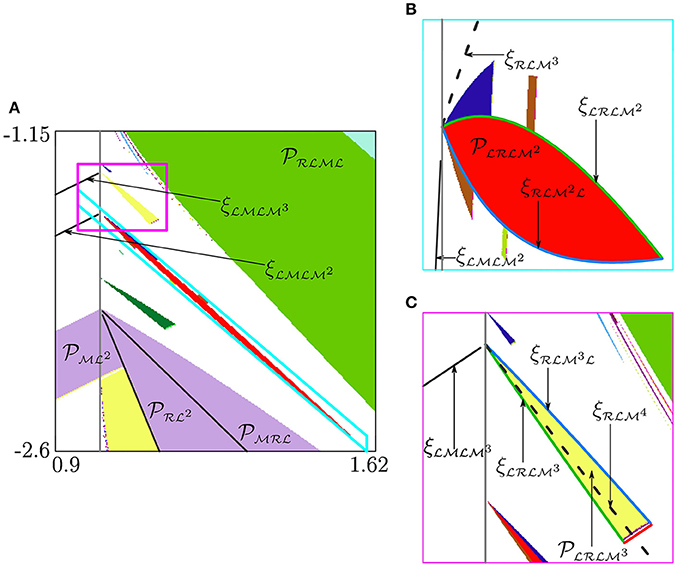
Figure 8. Stabilization of U-sequence cycles. Panels (B,C) are the enlargements of the areas marked in (A) by blue and magenta lines, respectively. The parameters are $a_{{L}}=0.57$, $a_{{R}}=0.2$, $d_{{L}}=0$, $d_{{R}}=1$.

To discover the origin of the tongues that are not D₀-prolongations of the STM structure, recall that for the skew tent map (12) even if the dynamics converges to a chaotic attractor, there exist also many periodic solutions that are unstable. These cycles appear due to BCBs or DFBs and according to a certain universal order with decreasing β. Namely, the symbolic sequences of these cycles form the so-called U-sequence where “U” stands for “universal,” since this order is common for a wide class of unimodal maps [19, 20]. Notice that usually U-sequence is described in terms of kneading sequences associated with superstable cycles (in the symbolic representation of which the symbol C related to the extremum of the function is omitted). The skew tent map obviously cannot have superstable cycles, and by using the term “U-sequence” we mean the order of appearance of the cycles in terms of their complete symbolic representation.

Another peculiarity of the skew tent map is that some blocks of the U-sequence appear simultaneously. For instance, crossing the DFB boundary ${\eta }_{{B}{A}}$ (or ${\eta }_{{B}}$ when α > 1) with decreasing β leads to immediate appearance of cycles with symbolic sequences being harmonics of ${B}$, defined in (18). Similar statement is true for a basic cycle ${{O}}_{{B}{{A}}^{n-1}}$, n ⩾ 3, that is, all its harmonics appear at the same parameter values (at the boundary ${\eta }_{{B}{{A}}^{n-1}}$).

In general, the U-sequence is constructed according to a certain iterative procedure and includes also the basic cycles. Detailed description of this construction procedure, as well as explanation of its peculiarities related to the skew tent map, is beyond the scopes of the current paper. Here we only explain how an unstable cycle whose symbolic sequence belongs to U-sequence may be “stabilized” when p enters D₀ crossing b₁ or b₂. For shortness we refer below to such cycles as U-sequence cycles.

Consider, for example, the region related to the 5-cycle observed in Figure 8A (see also the enlargement in Figure 8B). For p ∈ D₁ the line ${\xi }_{{L}{M}{L}{{M}}^2}$ denotes the fold BCB, at which two unstable 5-cycles are born: the cycle ${{O}}_{{L}{M}{L}{{M}}^2}$ and its complementary cycle ${{O}}_{{{M}}^2{L}{{M}}^2}$. The condition related to this bifurcation is

$\begin{array}{ll}{f}^5(d_{{L}})=f_{{L}{M}{L}{{M}}^2}(d_{{L}})\equiv f_{{{M}}^2{L}{{M}}^2}(d_{{L}})=d_{{L}}.& (53)\end{array}$

In fact, (53) defines two different BCB conditions which are equivalent due to the continuity of f, that is, $f_{{L}}(d_{{L}})=f_{{M}}(d_{{L}})$. This explains why the two cycles (which coincide at the bifurcation moment) appear simultaneously and why their symbolic sequences after the bifurcation differ by a single symbol.

For $p\in {\xi }_{{L}{M}{L}{{M}}^2}\cap b_1$ the condition (53) can be rewritten taking into account that $f(d_{{L}})=d_{{R}}$:

$\begin{array}{ll}{f}^5(d_{{L}})=f^4(d_{{R}})=f_{{M}{L}{{M}}^2}(d_{{R}})\equiv f_{{R}{L}{{M}}^2}(d_{{R}})=d_{{L}},& (54)\end{array}$

since $f_{{M}}(d_{{R}})=f_{{R}}(d_{{R}})$. Applying f one more time to (54), and using again the continuity property of f, we get

$\begin{array}{l}{f}^5(d_{{R}})=f_{{M}{L}{{M}}^2{L}}(d_{{R}})\equiv f_{{R}{L}{{M}}^2{L}}(d_{{R}})\equiv f_{{M}{L}{{M}}^2{M}}(d_{{R}})\\ \equiv f_{{R}{L}{{M}}^2{M}}(d_{{R}})=d_{{R}}(=f(d_{{L}})).& (55)\end{array}$

Similarly to (53), the equalities (55) define four BCB conditions that, nevertheless, are equivalent for $p\in {\xi }_{{L}{M}{L}{{M}}^2}\cap b_1$. Notice that in (55) the BCB conditions depend on $d_{{R}}$, in contrast to (53) where they depend on $d_{{L}}$. This is similar to how conditions of homoclinic bifurcations change when the parameter point p moves from D₁ to D₀ (as described in Section 5).

Now, for p ∈ D₀ not all the BCB conditions (55) remain equivalent. Moreover, the two cycles ${{O}}_{{L}{M}{L}{{M}}^2}$ and ${{O}}_{{{M}}^2{L}{{M}}^2}$ do not appear simultaneously for p ∈ D₀. Instead, each of them creates a complementary pair with one of the two new cycles having a single point in $I_{{R}}$ (and, thus, existing only for p ∈ D₀). Namely, the cycle ${{O}}_{{L}{M}{L}{{M}}^2}$ is now complementary to ${{O}}_{{L}{R}{L}{{M}}^2}$, while ${{O}}_{{{M}}^2{L}{{M}}^2}$ is complementary to ${{O}}_{{M}{R}{L}{{M}}^2}$. Clearly, the BCB conditions for the two cycles making a pair are equivalent, that is,

$\begin{array}{l}{f}_{{M}{L}{{M}}^2{L}}(d_{{R}})\equiv f_{{R}{L}{{M}}^2{L}}(d_{{R}})=d_{{R}},\\ f_{{M}{L}{{M}}^2{M}}(d_{{R}})\equiv f_{{R}{L}{{M}}^2{M}}(d_{{R}})=d_{{R}}.& (56)\end{array}$

However, the related bifurcation is not necessarily fold BCB.

Let us describe in more detail the BCBs related to four mentioned 5-cycles. With decreasing ${\mu }_{{R}}$ (for the other parameter values as in Figure 8) they appear in the following order. First, the two unstable cycles ${{O}}_{{{M}}^2{L}{{M}}^2}$ and ${{O}}_{{M}{R}{L}{{M}}^2}$ are born due to the fold BCB ${\xi }_{{R}{L}{{M}}^3}$ (dashed curve). Then there occurs the BCB ${\xi }_{{L}{R}{L}{{M}}^2}$ (green curve), at which the point $x_{{M}{R}{L}{{M}}^2}$ of ${{O}}_{{M}{R}{L}{{M}}^2}$ moves from the middle partition $I_{{M}}$ to the left one $I_{{L}}$. Hence, the stable cycle ${{O}}_{{L}{R}{L}{{M}}^2}$ appears. Finally, the point of ${{O}}_{{L}{R}{L}{{M}}^2}$ located in the right partition $I_{{R}}$ moves to the middle partition $I_{{M}}$ due to the other BCB ${\xi }_{{R}{L}{{M}}^2{L}}$ creating the unstable cycle ${{O}}_{{{M}}^2{L}{{M}}^2}$. The region ${{P}}_{{L}{R}{L}{{M}}^2}$ is then confined by ${\xi }_{{R}{L}{{M}}^2{L}}$ and ${\xi }_{{L}{R}{L}{{M}}^2}$. For ${\mu }_{{R}}$ being below ${\xi }_{{R}{L}{{M}}^2{L}}$ the two unstable cycles ${{O}}_{{L}{M}{L}{{M}}^2}$ and ${{O}}_{{{M}}^2{L}{{M}}^2}$ continue to exist.

We also remark that the region ${{P}}_{{L}{R}{L}{{M}}^2}$ has fins similarly to PA-regions. The mechanism of their creation is the same. Indeed, at the BCB boundary of ${{P}}_{{L}{R}{L}{{M}}^2}$ related to collision of the cycle with $d_{{L}}$/$d_{{R}}$, the map f⁵ is locally (in the neighborhood of $d_{{L}}$/$d_{{R}}$) topologically equivalent to the skew tent map g_α,β,1 with $\alpha =a_{{L}}^2{a}_{{M}}^2{a}_{{R}}$ and $\beta =a_{{L}}{a}_{{M}}^3{a}_{{R}}$/$\beta =a_{{L}}{a}_{{M}}^3$. Crossing transversally this BCB boundary may lead to appearance of a stable 5k-cycle, k ⩾ 1 (cf. Section 4.2). Existence of fins and their number depends on the parameter values.

The scenario due to that the region ${{P}}_{{L}{R}{L}{{M}}^2}$ occurs corresponds to what we call the “stabilization” of a U-sequence cycle. That is, for p ∈ D₁ the U-sequence cycle ${{O}}_{\sigma }$ is unstable (except for the basic cycles ${{O}}_{{M}{{L}}^{n-1}}$, n ⩾ 2, which can be stable). When p crosses b₁ entering D₀ a new cycle ${{O}}_{\sigma \prime }$ (among the others) is born. The symbolic sequence σ′ differs from σ by a single symbol. Namely, the symbol ${M}$ corresponding to the rightmost point of ${{O}}_{\sigma }$ is replaced by ${R}$ in σ′. If the slope $a_{{R}}$ is small enough, the cycle ${{O}}_{\sigma \prime }$ is stable.

The region related to a 6-cycle observed as well in Figure 8A has the same origin, though it looks somewhat unlike ${{P}}_{{L}{R}{L}{{M}}^2}$. Let us consider it in more detail and explain why it has different form. For p ∈ D₁ due to the BCB ${\xi }_{{L}{M}{L}{{M}}^3}$ the two unstable 6-cycles ${{O}}_{{L}{M}{L}{{M}}^3}$ and ${{O}}_{{{M}}^2{L}{{M}}^3}$ appear. Similarly to the case considered above (of the 5-cycle), for p ∈ D₀ there are two more 6-cycles: ${{O}}_{{L}{R}{L}{{M}}^3}$ (stable) and ${{O}}_{{M}{R}{L}{{M}}^3}$ (unstable). However, in contrast to the previous case, the sequence of bifurcations occurring with decreasing ${\mu }_{{R}}$ is different. First, the fold BCB ${\xi }_{{R}{L}{{M}}^3{L}}$ occurs giving rise to the stable cycle ${{O}}_{{L}{R}{L}{{M}}^3}$ and the unstable one ${{O}}_{{L}{M}{L}{{M}}^3}$. Next, the two unstable cycles ${{O}}_{{M}{R}{L}{{M}}^3}$ and ${{O}}_{{{M}}^2{L}{{M}}^3}$ appear due to the fold BCB ${\xi }_{{R}{L}{{M}}^4}$. Finally, ${{O}}_{{L}{R}{L}{{M}}^3}$ (stable) and ${{O}}_{{M}{R}{L}{{M}}^3}$ (unstable) disappear at ${\xi }_{{L}{R}{L}{{M}}^3}$. Notice that the region ${{P}}_{{L}{R}{L}{{M}}^3}$ (differently from ${{P}}_{{L}{R}{L}{{M}}^2}$) has one more boundary ${\eta }_{{L}{R}{L}{{M}}^3}$ that corresponds to the DFB of the related cycle.

The other regions emerging from b₁ and not belonging to PA or fin structures are of the same nature as the two regions described above. Notice that, for a U-sequence cycle ${{O}}_{{L}{M}\sigma }$, the higher is its period, the more of its points are located in $I_{{M}}$. Thus, to observe for p ∈ D₀ the region ${{P}}_{{L}{R}\sigma }$ corresponding to the “stabilized” version of ${{O}}_{{L}{M}\sigma }$, the value $a_{{R}}$ should be small enough. In the limit case $a_{{R}}=0$, for every U-sequence cycle there exists the related periodicity region in D₀ (see Figure 9), since the multiplier of ${{O}}_{{L}{R}\sigma }$ equals zero. Clearly, all these regions have only BCB boundaries and extend to infinite values of ${\mu }_{{L}}$, ${\mu }_{{R}}$.

FIGURE 9

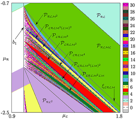
Figure 9. Periodicity regions related to “stabilized” versions of U-sequence cycles in the limit case $a_{{R}}=0$.

6. Chaoticity Regions Surrounding the Period Adding and the Fin Structures

In Section 4.1 we have recalled how to obtain boundaries of PA-regions. There are chaoticity regions adjacent to them, and now we discuss how their boundaries can be derived using the skew tent map. As an example, Figure 10 shows the structure of chaoticity regions close to the BCB boundary ${\xi }_{{L}{R}}$ of the PA-region ${{P}}_{{L}{R}}$. One can observe here two hatched domains. The first one, denoted $D_{st}^{{L},{L}{R}}$, is contiguous to the PA-region ${{P}}_{{L}{R}}$ along the boundary ${\xi }_{{L}{R}}$. For $p\in D_{st}^{{L},{L}{R}}$ the map f² is locally topologically conjugate to the skew tent map. Hence, the bifurcation structure can be described by applying directly the results known for the skew tent map.

FIGURE 10

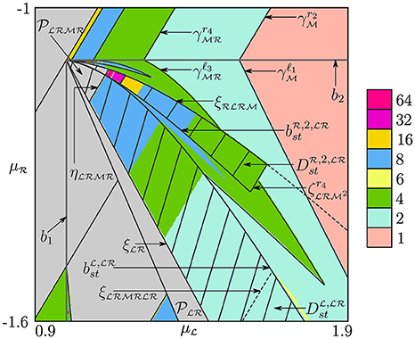
Figure 10. Bifurcation structure related to chaoticity regions associated with the PA-region ${{P}}_{{L}{R}}$ and its left 2 · 2-fin ${{P}}_{{L}{R}{M}{R}}$. The regions $D_{st}^{{L},{L}{R}}$ and $D_{st}^{{R},2,{L}{R}}$ are shown dashed.

In general, in the neighborhood of the boundary ${\xi }_{\sigma }^{d_{{L}}}$/${\xi }_{\sigma }^{d_{{R}}}$ of every PA-region ${{P}}_{\sigma }$ associated with an n-cycle ${{O}}_{\sigma }$, there exist domains denoted $D_{st}^{{L},\sigma }$/$D_{st}^{{R},\sigma }$, respectively, such that for related parameter values the iterate fⁿ is locally (in the neighborhood of $d_{{L}}$/$d_{{R}}$) topologically conjugate to the skew tent map.

The second hatched domain in Figure 10, denoted $D_{st}^{{R},2,{L}{R}}$, is located in the neighborhood of the boundary ${\xi }_{{R}{L}{R}{M}}$ of the left 2 · 2-fin region ${{P}}_{{L}{R}{M}{R}}$. In general, let us consider an arbitrary PA-region ${{P}}_{\sigma }$, related to the n-cycle ${{O}}_{\sigma }$, and its left/right k · n-fin ${{P}}_{\tau }$. In the neighborhood of the BCB boundary ${\xi }_{\tau }^{d_{{R}}}$/${\xi }_{\tau }^{d_{{L}}}$, respectively, there exists a domain $D_{st}^{{R},k,\sigma }$/$D_{st}^{{L},k,\sigma }$ such that the restriction of f^kn to its absorbing interval is topologically conjugate to the skew tent map.

6.1. Homoclinic Bifurcation Boundaries in $D_{st}^{{L},\sigma }$

We consider first the trunk region ${{P}}_{{L}{R}}$ and sub-domain $D_{st}^{{L},{L}{R}}$ contiguous to it along the boundary ${\xi }_{{L}{R}}$. Clearly, both points of the 2-cycle ${{O}}_{{L}{R}}=\left\{x_{{L}{R}},x_{{R}{L}}\right\}$ are fixed points for the second iterate f², and at $p\in {\xi }_{{L}{R}}$ the point $x_{{L}{R}}$ collides with $d_{{L}}$. The resulting dynamics caused by this collision depends on the slopes of f² at both sides of $d_{{L}}$ at the bifurcation moment. In the neighborhood of the border point the map f² is defined as (see Figure 11)

$f^2(x)\equiv \{\begin{array}{l}{f}_{{L}{R}},f_{{L}}^{-1}(d_{{R}})<x⩽d_{{L}},\hfill \\ f_{{M}{R}},d_{{L}}<x⩽f_{{M}}^{-1}(d_{{R}}),\hfill \end{array}$

where $f_{{L}}^{-1}(d_{{R}})=(d_{{R}}-{\mu }_{{L}})/a_{{L}}$, $f_{{M}}^{-1}(d_{{R}})=(d_{{R}}-{\mu }_{{M}})/a_{{M}}$. If the condition

$\begin{array}{ll}{f}_{{L}{R}}(d_{{L}})<f_{{M}}^{-1}(d_{{R}})& (57)\end{array}$

is satisfied, then f² has a local absorbing interval $J=\left[f_{{M}{R}}^2(d_{{L}}),f_{{M}{R}}(d_{{L}})\right]$, on which f² is topologically conjugate to the skew tent map (12) with $\alpha =a_{{L}}{a}_{{R}}$ and $\beta =a_{{M}}{a}_{{R}}$. The parameter region for that the conjugacy takes place is given as

$\begin{array}{l}{D}_{st}^{{L},{L}{R}}=\left\{p\in D_0:x_{{L}{R}}>d_{{L}},f_{{M}{R}}({l})<d_{{R}}\right\}=\\ \left\{\begin{array}{l}\begin{array}{l}p\in D_0:{\mu }_{{L}}>-\frac{{\mu }_{{R}}}{a_{{R}}}+\frac{1-a_{{R}}{a}_{{L}}}{a_{{R}}}{d}_{{L}},\\ a_{{R}}{a}_{{M}}{l}+a_{{R}}{\mu }_{{M}}+{\mu }_{{R}}<d_{{R}}\end{array}\hfill \end{array}\right\}.& (58)\end{array}$

FIGURE 11

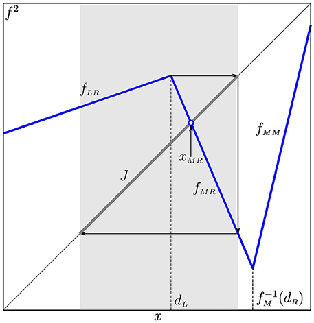
Figure 11. The local absorbing interval J of f² including $d_{{L}}$ for $p\in D_{st}^{{L},{L}{R}}$.

It is located between two boundaries, namely, ${\xi }_{{L}{R}}$ and

$\begin{array}{ll}{b}_{st}^{{L},{L}{R}}=\left\{p\in D_0:f_{{M}{R}}(\ell )=d_{{R}}\right\},& (59)\end{array}$

which follows from the equality $f_{{L}{R}}(d_{{L}})=f_{{M}}^{-1}(d_{{R}})$.

For $p\in D_{st}^{{L},{L}{R}}$ expressions for all bifurcation boundaries are derived directly from the related expressions known for the skew tent map (cf. Section 3).

Similarly, for an arbitrary PA-region ${{P}}_{\sigma }$ related to an n-cycle ${{O}}_{\sigma }$, n = |σ|, let $\sigma ={L}{\sigma }_1{R}{\sigma }_2$, where the symbolic sequences σ₁ and σ₂ are such that the point $x_{{L}{\sigma }_1{R}{\sigma }_2}$/$x_{{R}{\sigma }_2{L}{\sigma }_1}$ collides with $d_{{L}}$/$d_{{R}}$ at the BCB boundary ${\xi }_{{L}{\sigma }_1{R}{\sigma }_2}$/${\xi }_{{R}{\sigma }_2{L}{\sigma }_1}$, respectively. For $p\in {{P}}_{\sigma }$ consider the map fⁿ, for which every point of ${{O}}_{\sigma }$ is a fixed point. Close to the boundary ${\xi }_{{L}{\sigma }_1{R}{\sigma }_2}$, two branches of fⁿ joining at the border point $d_{{L}}$ are

$f^n(x)\equiv \{\begin{array}{l}{f}_{{L}{\sigma }_1{R}{\sigma }_2},\stackrel{⌣}{d}<x⩽d_{{L}},\hfill \\ f_{{M}{\sigma }_1{R}{\sigma }_2},d_{{L}}<x⩽\overline{d}.\hfill \end{array}$

Here $\stackrel{⌣}{d}$ and $\bar{d}$ are preimages of $d_{{R}}$, such that $f_{{L}{\sigma }_1}(\stackrel{⌣}{d})=d_{{R}}$ and $f_{{M}{\sigma }_1}(\bar{d})=d_{{R}}$. As before it can be shown that as long as

$\begin{array}{ll}{f}^n(d_{{L}})\equiv f_{{L}{\sigma }_1{R}{\sigma }_2}(d_{{L}})<\bar{d}& (60)\end{array}$

there exists a local absorbing interval

$\begin{array}{ll}J=\left[f_{{M}{\sigma }_1{R}{\sigma }_2}^2(d_{{L}}),f_{{M}{\sigma }_1{R}{\sigma }_2}(d_{{L}})\right]& (61)\end{array}$

such that the restriction $f^n{|}_J$ is topologically conjugate to the skew tent map g with the slopes $\alpha =a_{{L}{\sigma }_1{R}{\sigma }_2}$ and $\beta =a_{{M}{\sigma }_1{R}{\sigma }_2}$. Here $a_{{L}{\sigma }_1{R}{\sigma }_2}$ and $a_{{M}{\sigma }_1{R}{\sigma }_2}$ are the slopes of the composite functions $f_{{L}{\sigma }_1{R}{\sigma }_2}$ and $f_{{M}{\sigma }_1{R}{\sigma }_2}$, respectively. Such a conjugacy persists until the parameter point p crosses the border $b_{st}^{{L},\sigma }$ given by the condition $f_{{L}{\sigma }_1{R}{\sigma }_2}(d_{{L}})=\bar{d}$, which is equivalent to $f_{{M}{\sigma }_1}(f_{{L}{\sigma }_1{R}{\sigma }_2}(d_{{L}}))=f_{{M}{\sigma }_1}(\bar{d})\equiv d_{{R}}$, i.e.,

$\begin{array}{ll}{b}_{st}^{{L},\sigma }=\left\{p\in D_0:f_{{\sigma }_1{R}{\sigma }_2{M}{\sigma }_1}(\ell )=d_{{R}}\right\}.& (62)\end{array}$

Hence, we can state the following

Proposition 3 ([17]). For $p\in D_{st}^{{L},\sigma }$, where the region

$\begin{array}{ll}{D}_{st}^{{L},\sigma }=\left\{p\in D_0:x_{{L}{\sigma }_1{R}{\sigma }_2}>d_{{L}},f_{{\sigma }_1{R}{\sigma }_2{M}{\sigma }_1}(\ell )<d_{{R}}\right\}& (63)\end{array}$

is confined by ${\xi }_{{L}{\sigma }_1{R}{\sigma }_2}$ and $b_{st}^{{L},\sigma }$ given in (62), the expressions for boundaries of periodicity regions (fins) and chaoticity regions can be obtained from the related expressions known for the skew tent map (62) substituting α by $a_{{L}{\sigma }_1{R}{\sigma }_2}$ and β by $a_{{M}{\sigma }_1{R}{\sigma }_2}$.

For instance, we consider the left k · n-fin ${{P}}_{\tau }$, $\tau ={M}{\sigma }_1{R}{\sigma }_2{({L}{\sigma }_1{R}{\sigma }_2)}^{k-1}$, k ⩾ 3, of the PA-region ${{P}}_{{L}{\sigma }_1{R}{\sigma }_2}$. This fin region represents the area located between three BCB boundaries: ${\xi }_{{L}{\sigma }_1{R}{\sigma }_2}$, ${\xi }_{{\tau }_i}^{d_{{L}}}$ (the point x_τi of the cycle ${{O}}_{\tau }$ collides with $d_{{L}}$), ${\xi }_{{\tau }_j}^{d_{{R}}}$ (the point x_τj of the cycle ${{O}}_{\tau }$ collides with $d_{{R}}$), and the DFB boundary η_τ. We remark that the boundaries ${\xi }_{{\tau }_i}^{d_{{L}}}$ and η_τ emerge from ${\xi }_{{L}{\sigma }_1{R}{\sigma }_2}$, as well as the boundaries between chaoticity regions adjacent to ${{P}}_{{L}{\sigma }_1{R}{\sigma }_2}$.

Analytic expressions for all these boundaries are derived by using the skew tent map. Boundaries of the fin region, ${\xi }_{{\tau }_i}^{d_{{L}}}$ and η_τ, are given in (41) and (40), respectively. Let us consider the merging and the expansion bifurcation boundaries confining chaoticity regions ${{Q}}_{2kn}$ and ${{Q}}_{kn}$. They can be obtained by applying map replacement technique to expressions for ${\gamma }_{{B}{{A}}^{k-1}}^{c_{2k}}$ (15) and ${\zeta }_{{B}{{A}}^{k-2}{B}}^{c_k}$ (17).

Namely, in (15) we substitute all symbols ${A}$ with symbolic sequence ${L}{\sigma }_1{R}{\sigma }_2$, all symbols ${B}$ with symbolic sequence ${M}{\sigma }_1{R}{\sigma }_2$, critical point c with $f_{{\sigma }_1{R}{\sigma }_2}(\ell )$, slope α with $a_{{L}{\sigma }_1{R}{\sigma }_2}$, and β with $a_{{M}{\sigma }_1{R}{\sigma }_2}$. Recall that $a_{{L}{\sigma }_1{R}{\sigma }_2}$ and $a_{{M}{\sigma }_1{R}{\sigma }_2}$ are the slopes of the composite functions $f_{{L}{\sigma }_1{R}{\sigma }_2}$ and $f_{{M}{\sigma }_1{R}{\sigma }_2}$, respectively. Expressing $a_{{L}{\sigma }_1{R}{\sigma }_2}$ and $a_{{M}{\sigma }_1{R}{\sigma }_2}$ in terms of the original parameters $a_{{L}}$, $a_{{M}}$, $a_{{R}}$ we obtain the merging bifurcation boundary ${\gamma }_{{M}{\sigma }_1{R}{\sigma }_2{({L}{\sigma }_1{R}{\sigma }_2)}^{k-1}}^{{\ell }_{2kn+n-1}}$ related to transition ${{Q}}_{2kn}\Rightarrow {{Q}}_{kn}$. Likewise, by applying the same replacement to (17) one gets the expansion bifurcation boundary ${\zeta }_{{M}{\sigma }_1{R}{\sigma }_2{({L}{\sigma }_1{R}{\sigma }_2)}^{k-2}{M}{\sigma }_1{R}{\sigma }_2}^{{\ell }_{kn+n-1}}$. In short this procedure can be represented by the following scheme:

$\begin{array}{lll}{\gamma }_{{B}{{A}}^{k-1}}^{c_{2k}}& {\displaystyle \underset{{A}\to {L}{\sigma }_1{R}{\sigma }_2{B}\to {M}{\sigma }_1{R}{\sigma }_2}{\overset{c\to f_{{\sigma }_1{R}{\sigma }_2}(\ell )}{\to }}}{\gamma }_{{M}{\sigma }_1{R}{\sigma }_2{({L}{\sigma }_1{R}{\sigma }_2)}^{k-1}}^{{\ell }_{2kn+n-1}}& (64\text{a})\end{array}$

$\begin{array}{lll}{\zeta }_{{B}{{A}}^{k-2}{B}}^{c_k}& {\displaystyle \underset{{A}\to {L}{\sigma }_1{R}{\sigma }_2{B}\to {M}{\sigma }_1{R}{\sigma }_2}{\overset{c\to f_{{\sigma }_1{R}{\sigma }_2}(\ell )}{\to }}}{\zeta }_{{M}{\sigma }_1{R}{\sigma }_2{({L}{\sigma }_1{R}{\sigma }_2)}^{k-2}{M}{\sigma }_1{R}{\sigma }_2}^{{\ell }_{kn+n-1}}.& (64\text{b})\end{array}$

For sake of shortness schemes of such kind are used below to describe similar replacement procedures.

To sum up we can state

Proposition 4 ([17]). Let the parameter point p move along the BCB boundary ${\xi }_{{L}{\sigma }_1{R}{\sigma }_2}$ starting from nk-fin region ${{P}}_{{M}{\sigma }_1{R}{\sigma }_2{({L}{\sigma }_1{R}{\sigma }_2)}^{k-1}}$, k ⩾ 3. Then p first crosses the DFB boundary ${\eta }_{{M}{\sigma }_1{R}{\sigma }_2{({L}{\sigma }_1{R}{\sigma }_2)}^{k-1}}$ (40) leading to 2kn-cyclic chaotic intervals ${{Q}}_{2kn}$, then the merging bifurcation boundary ${\gamma }_{{M}{\sigma }_1{R}{\sigma }_2{({L}{\sigma }_1{R}{\sigma }_2)}^{k-1}}^{{\ell }_{2kn+n-1}}$ (64a) implying the transition ${{Q}}_{2kn}\Rightarrow {{Q}}_{kn}$, and finally, the expansion bifurcation boundary ${\zeta }_{{M}{\sigma }_1{R}{\sigma }_2{({L}{\sigma }_1{R}{\sigma }_2)}^{k-2}{M}{\sigma }_1{R}{\sigma }_2}^{{\ell }_{kn+n-1}}$ (64b) leading to ${{Q}}_{kn}\Rightarrow {{Q}}_n$.

The case k = 2 is particular. Since a 2n-fin cycle corresponds to the 2-cycle of the skew tent map g, its DFB leads to the appearance of 2^m·n-cyclic chaotic intervals, where m ⩾ 2 depends on $a_{{L}}$, $a_{{R}}$. The cascade of the subsequent merging bifurcations is obtained from (20) applying the same replacement as in (64). In Figure 12 an example of this cascade observed inside the domain $D_{st}^{{L},{L}{R}}$ is shown, located close to the left 2 · 2-fin region ${{P}}_{{L}{R}{M}{R}}$ of the trunk region ${{P}}_{{L}{R}}$. One can see three merging bifurcation boundaries, namely, ${\gamma }_{{M}{R}{L}{R}{({M}{R})}^2}^{{\ell }_{17}}$, ${\gamma }_{{M}{R}{L}{R}}^{{\ell }_9}$, and ${\gamma }_{{M}{R}}^{{\ell }_5}$ leading to the transitions ${{Q}}_{2·8}\Rightarrow {{Q}}_{2·4}\Rightarrow {{Q}}_{2·2}\Rightarrow {{Q}}_2$, respectively. To get the expression for ${\gamma }_{{M}{R}{L}{R}{({M}{R})}^2}^{{\ell }_{17}}$ the following replacement

$\begin{array}{l}{\gamma }_{{B}{A}{{B}}^2}^{c_8}{\displaystyle \underset{{A}\to {L}{R}{B}\to {M}{R}}{\overset{c\to f_{{R}}(\ell )}{\to }}}{\gamma }_{{M}{R}{L}{R}{({M}{R})}^2}^{{\ell }_{17}}\end{array}$

can be used. In this way we obtain

$\begin{array}{l}{\gamma }_{{M}{R}{L}{R}{({M}{R})}^2}^{{\ell }_{17}}=\left\{p\in D_0:a_{{L}{R}}^2{a}_{{M}{R}}^6+\frac{a_{{L}{R}}}{a_{{M}{R}}}-1=0\right\}\\ =\left\{p\in D_0:a_{{L}}^2{a}_{{M}}^6{a}_{{R}}^8+\frac{a_{{M}}}{a_{{L}}}-1=0\right\}.& (65)\end{array}$

The expressions for the other two boundaries

$\begin{array}{ll}{\gamma }_{{M}{R}{L}{R}}^{{\ell }_9}=\left\{p\in D_0:a_{{L}}^2{a}_{{M}}^2{a}_{{R}}^4+\frac{a_{{L}}}{a_{{M}}}-1=0\right\},& (66\text{a})\end{array}$

$\begin{array}{ll}{\gamma }_{{M}{R}}^{{\ell }_5}=\left\{p\in D_0:a_{{M}}^2{a}_{{R}}^2+\frac{a_{{M}}}{a_{{L}}}-1=0\right\}& (66\text{b})\end{array}$

can be obtained by the same replacement.

FIGURE 12

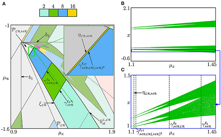
Figure 12. (A) Bifurcation structure of the region $D_{st}^{{L},{L}{R}}$. Bifurcation diagram (B) along the arrow shown green in (A) and its enlargement (C).

We have described above bifurcations of cyclic chaotic intervals and the related boundaries in the neighborhood of ${\xi }_{\sigma }^{d_{{L}}}$ of a PA-region ${{P}}_{\sigma }$. To obtain similar bifurcation boundaries in the neighborhood of ${\xi }_{\sigma }^{d_{{R}}}$ one can swap symbols ${L}$ and ${R}$ as well as interchange the critical points ℓ and r in all analytic expressions.

6.2. Homoclinic Bifurcation Boundaries in $D_{st}^{{R},K,\sigma }$

In this section we describe another parameter domain $D_{st}^{{R},k,\sigma }$, mentioned above, which is located in the neighborhood of an arbitrary left fin region of a PA-region ${{P}}_{\sigma }$. To describe bifurcation structure of $D_{st}^{{R},k,\sigma }$ we again use conjugacy with skew tent map and map replacement technique.

As the first example let us consider the left 2 · 2-fin region ${{P}}_{{L}{R}{M}{R}}$ of the trunk region ${{P}}_{{L}{R}}$ (see Figure Figures 12A). As explained in Section 4.2 the fin region ${{P}}_{{L}{R}{M}{R}}$ has the BCB boundary ${\xi }_{{R}{L}{R}{M}}$ related to the collision of the cycle ${{O}}_{{L}{R}{M}{R}}$ with the border $d_{{R}}$.

In Figure 13 we show the plot of f⁴ on the interval including the border point $d_{{R}}$ for parameter values located in the neighborhood of ${\xi }_{{R}{L}{R}{M}}$. The two linear pieces of f⁴ adjoining at $d_{{R}}$ are defined as

$f^4(x)\equiv \{\begin{array}{l}{f}_{{M}{L}{R}{M}},f_{{M}}^{-1}(d_{{L}})⩾x⩽d_{{R}},\hfill \\ f_{{R}{L}{R}{M}},d_{{R}}<x⩽f_{{R}}^{-1}(d_{{L}}),\hfill \end{array}$

where $f_{{M}}^{-1}(d_{{L}})=(d_{{L}}-{\mu }_{{M}})/a_{{M}}$, $f_{{R}}^{-1}(d_{{L}})=(d_{{L}}-{\mu }_{{R}})/a_{{R}}$. If the conditions

$\begin{array}{ll}{f}_{{R}{L}{R}{M}}(d_{{R}})<f_{{R}}^{-1}(d_{{L}}),& (67\text{a})\end{array}$

$\begin{array}{ll}{f}_{{R}{L}{R}{M}}^2(d_{{R}})>x_{{M}{L}{R}{M}}& (67\text{b})\end{array}$

are held, then there exists a local absorbing interval

$\begin{array}{ll}J=\left[f_{{R}{L}{R}{M}}^2(d_{{R}}),f_{{R}{L}{R}{M}}(d_{{R}})\right]& (68)\end{array}$

for f⁴. The restriction $f^4{|}_J$ is topologically conjugate to the skew tent map g with the slopes $\alpha =a_{{L}}{a}_{{M}}^2{a}_{{R}}$ and $\beta =a_{{L}}{a}_{{M}}{a}_{{R}}^2$.

FIGURE 13

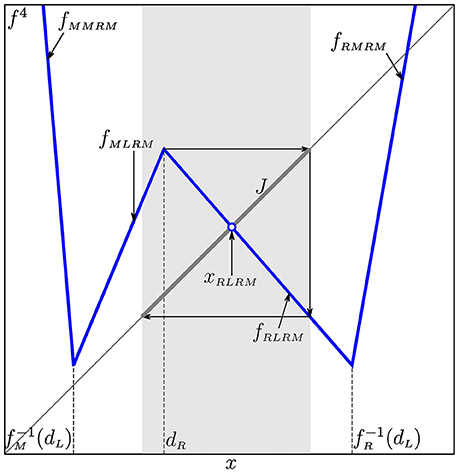
Figure 13. The local absorbing interval J of f⁴ including $d_{{R}}$ for $p\in D_{st}^{{R},2,{L}{R}}$.

Taking into account that $f_{{R}}(f_{{R}{L}{R}{M}}(d_{{R}}))\equiv f_{{L}{R}{M}{R}}(r)$, $f_{{R}{L}{R}{M}}^2(d_{{R}})=f_{{L}{R}{M}}(f_{{R}{L}{R}{M}}(r))$, and $x_{{M}{L}{R}{M}}=f_{{L}{R}{M}}(x_{{L}{R}{{M}}^2})$, the conditions (67) can be written as

$\begin{array}{ll}{f}_{{L}{R}{M}{R}}(r)<d_{{L}},& (69\text{a})\end{array}$

$\begin{array}{ll}{f}_{{L}{R}{M}{R}}(r)>x_{{L}{R}{{M}}^2}.& (69\text{b})\end{array}$

The conjugacy between $f^4{|}_J$ and g holds in the parameter region $D_{st}^{{R},2,{L}{R}}$ confined by the BCB boundary ${\xi }_{{R}{L}{R}{M}}$, the boundary

$\begin{array}{ll}{b}_{st}^{{R},2,{L}{R}}=\left\{p\in D_0:f_{{L}{R}{M}{R}}(r)=d_{{L}}\right\},& (70)\end{array}$

and the boundary

$\begin{array}{ll}{\zeta }_{{L}{R}{{M}}^2}^{r_4}=\left\{p\in D_0:f_{{L}{R}{M}{R}}(r)=x_{{L}{R}{{M}}^2}\right\}.& (71)\end{array}$

Note that for the map f the boundary (71) corresponds to an expansion bifurcation leading from ${{Q}}_4$ to ${Q}$. Thus, the region $D_{st}^{{R},2,{L}{R}}$ is defined as

$\begin{array}{l}{D}_{st}^{{R},2,{L}{R}}=\{p\in D_0:x_{{R}{L}{R}{M}}>d_{{R}},f_{{L}{R}{M}{R}}(r)<d_{{L}},\\ f_{{L}{R}{M}{R}}(r)>x_{{L}{R}{{M}}^2}\}.& (72)\end{array}$

Figure 14A presents the region $D_{st}^{{R},2,{L}{R}}$, where one can observe chaoticity regions ${{Q}}_{2^m}$, $m=\overline{2,6}$. The bifurcation boundaries separating these regions are related to transitions ${{Q}}_{2^m}\Rightarrow {{Q}}_{2^{m-1}}$. To get expressions for these boundaries we use map replacement technique. Namely, we take the corresponding formulae (20) known for the skew tent map and apply the following replacement:

${\gamma }_{{\rho }_j}^{c_{2^{j+1}}}\underset{{A}\to {M}{L}{R}{M}B\to {R}{L}{R}{M}}{\overset{c\to f_{{L}{R}{M}}(r)}{\to }}{\gamma }_{{\tau }_j}^{r_{2^{j+3}+3}}.(73)$

Here the symbolic sequence τ_j, j ⩾ 0, is derived from the harmonic ρ_j (18) by substituting ${M}{L}{R}{M}$ instead of ${A}$ and ${R}{L}{R}{M}$ instead of ${B}$.

FIGURE 14

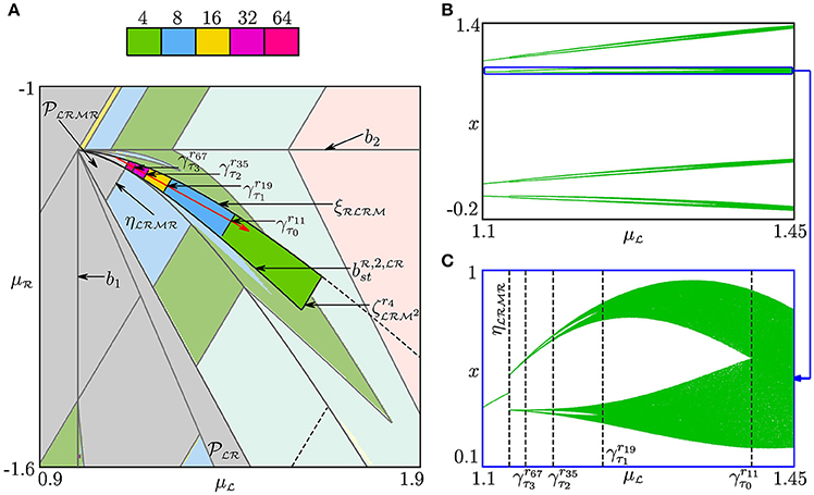
Figure 14. (A) Bifurcation structure of the region $D_{st}^{{R},2,{L}{R}}$. Bifurcation diagram (B) along the arrow shown red in (A) and its enlargement (C).

Summing up we can describe $D_{st}^{{R},2,{L}{R}}$ in the following way. The region $D_{st}^{{R},2,{L}{R}}\backslash {{P}}_{{L}{R}{M}{R}}$ consists of t + 1 chaoticity regions ${{C}}_{4·2^j}$, $j=\overline{0,t}$, where t ⩾ 1 depends on $a_{{L}}$, $a_{{R}}$. If the parameter point p crosses the boundary ${\gamma }_{{\tau }_j}^{r_{2^{j+3}+3}}$ between the chaoticity regions ${{C}}_{2^{j+1}}$ and ${{C}}_{2^j}$, given by

$\begin{array}{l}{\gamma }_{{\tau }_j}^{r_{2^{j+3}+3}}=\{p\in D_{st}^{{L}}:a_{{L}}^{2({\delta }_j+{\delta }_{j+1})}{a}_{{M}}^{2(2{\delta }_j+{\delta }_{j+1})}{a}_{{R}}^{2({\delta }_j+2{\delta }_{j+1})}\\ +{\left(\frac{a_{{M}}}{a_{{R}}}\right)}^{{(-1)}^{j+1}}-1=0\},j=\overline{0,t-1},\end{array}$

then the merging bifurcation ${{C}}_{2^{j+1}}\Rightarrow {{C}}_{2^j}$ takes place. Here ${\delta }_j=(2^j-{(-1)}^j)/3$. In Figure 14A the merging bifurcation boundaries ${\gamma }_{{\tau }_3}^{r_{67}}$, ${\gamma }_{{\tau }_2}^{r_{35}}$, ${\gamma }_{{\tau }_1}^{r_{19}}$, and ${\gamma }_{{\tau }_0}^{r_{11}}$ are shown. See also 1D bifurcation diagrams in Figures 14B,C.

In a similar way we characterize the region $D_{st}^{{R},k,\sigma }$, related to the boundary ${\xi }_{\tau }^{d_{{R}}}$ of the left k · n-fin ${{P}}_{\tau }$, $\tau ={({L}{\sigma }_1{R}{\sigma }_2)}^{k-1}{M}{\sigma }_1{R}{\sigma }_2$, of the trunk region ${{P}}_{{L}{\sigma }_1{R}{\sigma }_2}$, k ⩾ 2, n ⩾ 2. In order to determine the branches of f^kn which are adjacent to one another at the border point, we rewrite the symbolic sequence associated with the fin cycle as follows:

$\begin{array}{ll}\tau \equiv \underset{\_}{{R}}{\sigma }_2{L}{\sigma }_1{({R}{\sigma }_2{L}{\sigma }_1)}^{k-3}{R}{\sigma }_2\underset{\_}{{L}}{\sigma }_1{R}{\sigma }_2{M}{\sigma }_1.& (74)\end{array}$

Here the underlined symbols $\underset{\_}{{R}}$ and $\underset{\_}{{L}}$ are associated with the points $x_{\underset{\_}{{R}}{\tau }_1}$, $x_{\underset{\_}{{L}}{\tau }_2}$ such that $x_{\underset{\_}{{R}}{\tau }_1}$ collides with $d_{{R}}$ at ${\xi }_{\tau }^{d_{{R}}}$, while $x_{\underset{\_}{{L}}{\tau }_2}$ collides with $d_{{L}}$ at ${\xi }_{\tau }^{d_{{L}}}$. We introduce the abbreviation

$\begin{array}{ll}{\omega }_1:={\sigma }_2{L}{\sigma }_1{({R}{\sigma }_2{L}{\sigma }_1)}^{k-3}{R}{\sigma }_2,{\omega }_2:={\sigma }_1{R}{\sigma }_2{M}{\sigma }_1& (75)\end{array}$

and rewrite the symbolic sequence (74) as ${R}{\omega }_1{L}{\omega }_2$. Then the points $x_{\underset{\_}{{R}}{\tau }_1}$ and $x_{\underset{\_}{{L}}{\tau }_2}$ become $x_{{R}{\omega }_1{L}{\omega }_2}$ and $x_{{L}{\omega }_2{R}{\omega }_1}$, respectively. Then in the neighborhood of $d_{{R}}$ the iterate f^kn is given by

$f^{kn}(x)\equiv \{\begin{array}{l}{f}_{{M}{\omega }_1{L}{\omega }_2},\tilde{d}<x⩽d_{{R}},\hfill \\ f_{{R}{\omega }_1{L}{\omega }_2},d_{{R}}<x<\widehat{d}\hfill \end{array}$

Here $\tilde{d}$ and $\widehat{d}$ are the preimages of $d_{{L}}$ such that

$\begin{array}{l}{f}_{{M}{\omega }_1}(\tilde{d})=d_{{L}},f_{{R}{\omega }_1}(\widehat{d})=d_{{L}}.\end{array}$

The map f^kn has in the neighborhood of $d_{{R}}$ a local absorbing interval

$\begin{array}{ll}J=\left[f_{{R}{\omega }_1{L}{\omega }_2}^2(d_{{R}}),f_{{R}{\omega }_1{L}{\omega }_2}(d_{{R}})\right]\subset \left[\tilde{d},\widehat{d}\right],& (76)\end{array}$

whenever the conditions

$\begin{array}{ll}{f}_{{R}{\omega }_1{L}{\omega }_2}(d_{{R}})<\widehat{d},f_{{R}{\omega }_1{L}{\omega }_2}^2(d_{{R}})>x_{{M}{\omega }_1{L}{\omega }_2},& (77)\end{array}$

are held. The restriction $f^{kn}{|}_J$ is topologically conjugate to the skew tent map g with

$\begin{array}{ll}\alpha =a_{{M}{\omega }_1{L}{\omega }_2},\beta =a_{{R}{\omega }_1{L}{\omega }_2}.& (78)\end{array}$

Taking into account that $f_{{R}{\omega }_1}(f_{{R}{\omega }_1{L}{\omega }_2}(d_{{R}}))\equiv f_{{\omega }_1{L}{\omega }_2{R}{\omega }_1}(r)$, $f_{{R}{\omega }_1{L}{\omega }_2}^2(d_{{R}})=f_{{\omega }_1{L}{\omega }_2}(f_{{\omega }_1{L}{\omega }_2{R}}(r))$, and $x_{{M}{\omega }_1{L}{\omega }_2}=f_{{\omega }_1{L}{\omega }_2}(x_{{\omega }_1{L}{\omega }_2{M}})$, the conditions (77) can be rewritten as

$\begin{array}{l}{f}_{{\omega }_1{L}{\omega }_2{R}{\omega }_1}(r)<d_{{L}},f_{{\omega }_1{L}{\omega }_2{R}}(r)>x_{{\omega }_1{L}{\omega }_2{M}}.\end{array}$

Therefore, the region $D_{st}^{{R},k,\sigma }$ in which the asymptotic dynamics of f can be studied by using the skew tent map g with the slopes given in (78), is confined by the BCB boundary ${\xi }_{{R}{\omega }_1{L}{\omega }_2}$, the border

$\begin{array}{ll}{b}_{st}^{{R},k,\sigma }=\left\{p\in D_0:f_{{\omega }_1{L}{\omega }_2{R}{\omega }_1}(r)=d_{{L}}\right\},& (79)\end{array}$

and the expansion bifurcation boundary

$\begin{array}{ll}{\zeta }_{{\omega }_1{L}{\omega }_2{M}}^{r_{nk}}=\left\{f_{{\omega }_1{L}{\omega }_2{R}}(r)=x_{{\omega }_1{L}{\omega }_2{M}}\right\}.& (80)\end{array}$

Accordingly, the region $D_{st}^{{R},k,\sigma }$ is given by

$\begin{array}{l}{D}_{st}^{{R},k,\sigma }=\{x_{{R}{\omega }_1{L}{\omega }_2}>d_{{R}},f_{{\omega }_1{L}{\omega }_2{R}{\omega }_1}(r)<d_{{L}},f_{{\omega }_1{L}{\omega }_2{R}}(r)\\ >x_{{\omega }_1{L}{\omega }_2{M}}\}.& (81)\end{array}$

To sum up we state

Proposition 5 ([17]). The region $D_{st}^{{R},k,\sigma }\backslash {{P}}_{{R}{\omega }_1{L}{\omega }_2}$ consists of t+1 chaoticity regions ${{C}}_{4·2^j}$, $j=\overline{0,t}$, where t ⩾ 1 depends on $a_{{L}}$, $a_{{R}}$. Each pair of contiguous chaoticity regions ${{C}}_{2^{j+1}}$ and ${{C}}_{2^j}$ is separated by the merging bifurcation boundary ${\gamma }_{{\tau }_j}^{r_{2^{j+1}nk+nk-1}}$ which is derived from (20) applying the following replacement

${\gamma }_{{\rho }_j}^{c_{2^{j+1}}}\underset{{A}\to {M}{\omega }_1{L}{\omega }_{2}B\to {R}{\omega }_1{L}{\omega }_2}{\overset{c\to f_{{\omega }_1{L}{\omega }_2}(r)}{\to }}{\gamma }_{{\tau }_j}^{r_{2^{j+1}nk+nk-1}},(82)$

where τ_j is obtained from the harmonic ρ_j (18) by replacing ${A}$ with ${M}{\omega }_1{L}{\omega }_2$ and ${B}$ with ${R}{\omega }_1{L}{\omega }_2$.

As before, to describe bifurcation structure of the parameter domain $D_{st}^{{L},k,\sigma }$, located in the neighborhood of an arbitrary right fin region of a PA-region ${{P}}_{\sigma }$, one can interchange ${L}$ and ${R}$ as well as the critical points ℓ and r in all analytic expressions.

6.3. Homoclinic Bifurcation Boundaries between $D_{st}^{{L},\sigma }$ and $D_{st}^{{R},K,\sigma }$

As one can see in Figure 10, between the regions $D_{st}^{{L},{L}{R}}$ and $D_{st}^{{R},2,{L}{R}}$ there are more bifurcation boundaries related to some homoclinic bifurcations. In contrast to the previous two sections, where chaotic intervals were associated with only one border point, $d_{{L}}$ or $d_{{R}}$, here we consider the case when chaotic intervals include both border points. This makes impossible direct usage of the results known for the skew tent map.

In Figures 15A,B we show the area between the regions $D_{st}^{{L},{L}{R}}$ and $D_{st}^{{R},2,{L}{R}}$. As one can observe there are several bifurcation boundaries issuing from the curves $b_{st}^{{L},{L}{R}}$ (59) and $b_{st}^{{R},2,{L}{R}}$ (70). Right below we briefly describe how these bifurcation boundaries can be derived.

FIGURE 15

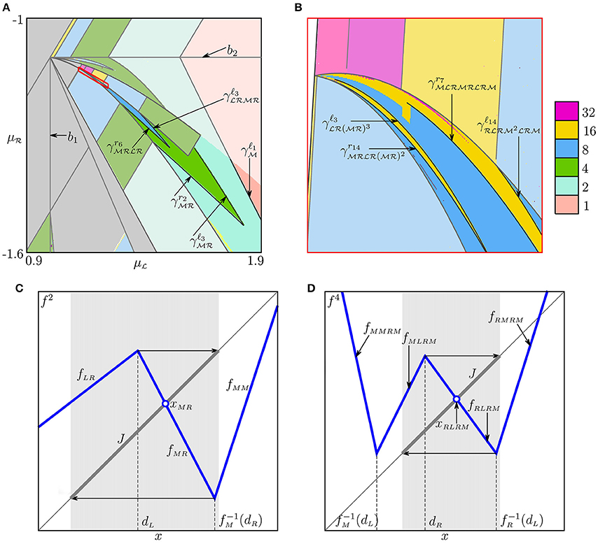
Figure 15. (A) Chaoticity regions located between $D_{st}^{{L},{L}{R}}$ and $D_{st}^{{R},2,{L}{R}}$; In (B) the region outlined red in (A) is shown enlarged. (C) Local absorbing interval of f² including $d_{{L}}$ for $p\notin D_{st}^{{L},{L}{R}}$ immediately after crossing $b_{st}^{{L},{L}{R}}$. (D) Local absorbing interval of f⁴ including $d_{{R}}$ for $p\notin D_{st}^{{R},2,{L}{R}}$ immediately after crossing $b_{st}^{{R},2,{L}{R}}$.

First, recall that $b_{st}^{{L},{L}{R}}$ is related to the condition $f_{{L}{R}}(d_{{L}})=f_{{M}}^{-1}(d_{{R}})$. Until $f_{{L}{R}}(d_{{L}})<f_{{M}}^{-1}(d_{{R}})$ (that is, inside $D_{st}^{{L},{L}{R}}$), the local absorbing interval J of f² includes only a single kink point $d_{{L}}$. Hence, $f^2{|}_J$ is defined by only two branches $f_{{L}{R}}$ and $f_{{M}{R}}$. When there holds the opposite inequality $f_{{L}{R}}(d_{{L}})>f_{{M}}^{-1}(d_{{R}})$, the absorbing interval J spreads over another kink point $f_{{M}}^{-1}(d_{{R}})$ (to the right of $d_{{L}}$) and becomes

$\begin{array}{l}J=\left[f_{{M}{R}}(f_{{M}}^{-1}(d_{{R}})),f_{{L}{R}}(d_{{L}})\right]=\left[r,f_{{R}}(\ell )\right]\ni f_{{M}}^{-1}(d_{{R}})\end{array}$

(see Figure 15C). Then $f^2{|}_J$ consists of three branches: $f_{{L}{R}}$, $f_{{M}{R}}$, and $f_{{M}{M}}$. This transformation is similar to the one described in Section 5.1 for the original map f, where the parameter point p crosses the border b₁. Hence, the bifurcation boundaries emerging from $b_{st}^{{L},{L}{R}}$ are of the same sort as D₀-prolongations. Applying the replacement

${\gamma }_{{\rho }_m}^{r_{2^{m+1}-1}}\underset{{L}\to {L}{R}{M}\to {M}{R}}{\overset{}{\to }}{\gamma }_{{\tau }_m}^{r_{2(2^{m+1}-1)}}(83)$

to (51), one obtains the related analytic expressions for the mentioned boundaries.

Then we apply the replacement

${\gamma }_{{\rho }_m^{\prime }}^{{\ell }_1}\underset{{L}\to {L}{R}{M}\to {M}{R}{R}\to {M}{M}}{\overset{\ell \to f_{{R}}(\ell )}{\to }}{\gamma }_{{\tau }_m^{\prime }}^{{\ell }_3}(84)$

to the additional boundary ${\gamma }_{{\rho }_m^{\prime }}^{{\ell }_1}$ (52). Here the sequences τ_m and ${\tau }_m^{\prime }$ are obtained from the sequences ρ_m and ${\rho }_m^{\prime }$, respectively, by replacing ${L}$ with ${L}{R}$ and ${M}$ with ${M}{R}$. Recall, that ρ_m consists of the symbols ${L}$ and ${M}$ and is the m-th harmonic of ${M}$ [see (18) with ${A}={L}$ and ${B}={M}$], while ${\rho }_m^{\prime }$ is obtained from ρ_m by shifting the first symbol ${M}$ to the end of the symbolic sequence. Note that in (83), r must be replaced by the value $f_{{M}{R}}(f_{{M}}^{-1}(d_{{R}}))\equiv f_{{R}}(d_{{R}})$ which coincides with r, and that is why the replacement for r is not necessary.

To illustrate the described procedure let us consider the boundary ${\gamma }_{{M}{R}}^{r_2}$ shown in Figure 15A which corresponds to the transition ${{Q}}_4\Rightarrow {{Q}}_2$. For f² this transition is associated with the merging of 2-cyclic chaotic intervals into a single chaotic interval. Thus, we can apply the replacement (83) to the expression for the D₀-prolongation ${\gamma }_{{M}}^{r_1}$ [i.e., (51) with m = 0] obtaining

$\begin{array}{ll}{\gamma }_{{M}{R}}^{r_2}=\left\{p\in D_0:f_{{L}{R}}(r)=x_{{M}{R}}\right\}.& (85)\end{array}$

Likewise, we derive the expression for the boundary ${\gamma }_{{M}{R}{L}{R}}^{r_6}$, which is associated with the transition ${{Q}}_8\Rightarrow {{Q}}_4$, by using the expression for the D₀-prolongation ${\gamma }_{{M}{L}}^{r_3}$ [i.e., (51) with m = 1]:

$\begin{array}{ll}{\gamma }_{{M}{R}{L}{R}}^{r_6}=\left\{p\in D_0:f_{{L}{R}{({M}{R})}^2}(r)=x_{{M}{R}{L}{R}}\right\}.& (86)\end{array}$

The other boundary ${\gamma }_{{L}{R}{M}{R}}^{{\ell }_3}$ associated with the same transition is derived from the boundary ${\gamma }_{{L}{M}}^{{\ell }_1}$ (52), m = 1, corresponding to another homoclinic bifurcation of ${{O}}_{{M}{L}}$. Applying (84) to ${\gamma }_{{L}{M}}^{{\ell }_1}$ we obtain

$\begin{array}{ll}{\gamma }_{{L}{R}{M}{R}}^{{\ell }_3}=\left\{p\in D_0:f_{{R}{M}{M}}(\ell )=x_{{L}{R}{M}{R}}\right\}.& (87)\end{array}$

In Figure 15B one can also see the boundaries ${\gamma }_{{M}{R}{L}{R}{({M}{R})}^2}^{r_{14}}$ and ${\gamma }_{{L}{R}{({M}{R})}^3}^{{\ell }_3}$, which correspond to the transition ${{Q}}_{16}\Rightarrow {{Q}}_8$. Setting m = 2 and applying the replacement (83) to (51) and the replacement (84) to (52) we get

$\begin{array}{l}{\gamma }_{{M}{L}{{M}}^2}^{r_7}\underset{{L}\to {L}{R}{M}\to {M}{R}}{\overset{}{\to }}{\gamma }_{{M}{R}{L}{R}{({M}{R})}^2}^{r_{14}},\\ {\gamma }_{{L}{{M}}^3}^{{\ell }_1}\underset{{L}\to {L}{R}{M}\to {M}{R}{R}\to {M}{M}}{\overset{\ell \to f_{{R}}(\ell )}{\to }}{\gamma }_{{L}{R}{({M}{R})}^3}^{{\ell }_3},\end{array}$

which implies

$\begin{array}{l}{\gamma }_{{M}{R}{L}{R}{({M}{R})}^2}^{r_{14}}\text{}=\{p\in D_0:f_{{L}{R}{({M}{R})}^2{({M}{R}{L}{R})}^2}(r)\\ \text{ }=x_{{M}{R}{L}{R}{({M}{R})}^2}\},& (88)\end{array}$

${\gamma }_{{L}{R}{({M}{R})}^3}^{{\ell }_3}\text{}=\text{}\left\{p\in D_0:f_{{R}{M}{M}}(\ell )=x_{{L}{R}{({M}{R})}^3}\right\}\text{}.(89)$

Analogously we consider the case where the parameter point p leaves the region $D_{st}^{{R},2,{L}{R}}$ crossing $b_{st}^{{R},2,{L}{R}}$. When $p\in D_{st}^{{R},2,{L}{R}}$ the condition $f_{{R}{L}{R}{M}}(d_{{R}})>f_{{R}}^{-1}(d_{{L}})$ is satisfied and the local absorbing interval J of f⁴ in the neighborhood of $d_{{R}}$ includes only two linear branches. Otherwise, the interval J spreads over the third branch $f_{{R}{M}{R}{M}}$ and becomes

$\begin{array}{l}J=[f_{{R}{L}{R}{M}}(f_{{R}}^{-1}(d_{{L}})),f_{{R}{L}{R}{M}}(d_{{R}})]\\ \equiv [f_{{R}{M}}(\ell ),f_{{L}{R}{M}}(r)]\ni f_{{R}}^{-1}(d_{{L}}).\end{array}$

See Figure 15D. Thus, for f⁴ crossing the border $b_{st}^{{R},2,{L}{R}}$ is similar to crossing b₁ for f. Consequently, the associated boundaries of chaoticity regions for $p\notin D_{st}^{{R},2,{L}{R}}$ can be derived as well from (51) and (52).

For example, the transition ${{Q}}_{16}\Rightarrow {{Q}}_8$ occurs at the boundaries ${\gamma }_{{M}{L}}^{r_3}$ and ${\gamma }_{{M}{L}{R}{M}{R}{L}{R}{M}}^{r_7}$. We use the expressions for ${\gamma }_{{M}{L}}^{r_3}$ (51) and ${\gamma }_{{L}{M}}^{{\ell }_1}$ (52) with m = 2 to compute these mentioned boundaries. It is enough to apply the following replacements:

$\begin{array}{l}{\gamma }_{{M}{L}}^{r_3}\underset{{L}\to {M}{L}{R}{M}{M}\to {R}{L}{R}{M}}{\overset{r\to f_{{R}{M}}(\ell )}{\to }}{\gamma }_{{R}{L}{R}{{M}}^2{L}{R}{M}}^{{\ell }_{14}},\\ {\gamma }_{{L}{M}}^{{\ell }_1}\underset{{L}\to {M}{L}{R}{M}{M}\to {R}{L}{R}{M}{R}\to {R}{M}{R}{M}}{\overset{\ell \to f_{{L}{R}{M}}(r)}{\to }}\\ {\gamma }_{{M}{L}{R}{M}{R}{L}{R}{M}}^{r_7}.& (90)\end{array}$

In this way we obtain

$\begin{array}{l}{\gamma }_{{R}{L}{R}{{M}}^2{L}{R}{M}}^{{\ell }_{14}}=\{p\in D_0:f_{{R}{M}{M}{L}{R}{M}{({R}{L}{R}{M})}^2}(\ell )\\ =x_{{R}{L}{R}{{M}}^2{L}{R}{M}}\},& (91\text{a})\end{array}$

$\begin{array}{l}{\gamma }_{{M}{L}{R}{M}{R}{L}{R}{M}}^{r_7}=\{p\in D_0:f_{{L}{({R}{M})}^3}(r)\\ =x_{{M}{L}{R}{M}{R}{L}{R}{M}}\}.& (91\text{b})\end{array}$

Regarding the merging bifurcation boundaries ${\gamma }_{{M}{R}}^{{\ell }_3}$ and ${\gamma }_{{M}}^{{\ell }_1}$ marked in Figure 15A, it can be shown that ${\gamma }_{{M}{R}}^{{\ell }_3}$ is the D₀-prolongation of ${\gamma }_{{M}{R}}^{r_4}\subset D_2$, and ${\gamma }_{{M}}^{{\ell }_1}$ is the D₀-prolongation of ${\gamma }_{{M}}^{r_2}\subset D_2$.

So far all bifurcation boundaries of the regions ${{C}}_2$, ${{C}}_4$, and ${{C}}_8$ related to the transitions ${{Q}}_8\Rightarrow {{Q}}_4\Rightarrow {{Q}}_2\Rightarrow {Q}$ are fully described. However, in Figure 15B one can see that the region ${{C}}_{16}$ has further boundaries different from those described above. We can suggest that the regions ${{C}}_{2^m}$, m ⩾ 4, have much more complicated form and may have other boundaries, whose description falls beyond the scopes of the current paper.

The above example can be generalized. That is, for an arbitrary PA-region ${{P}}_{\sigma }$ we consider the are located between the regions $D_{st}^{{L},\sigma }$ and $D_{st}^{{R},k,\sigma }$, k ⩾ 2. The bifurcation boundaries inside this area are derived in a similar way by using the relevant replacements (for details see [17]).

7. Conclusions

In this work we carry on studying asymptotic dynamics of a 1D continuous bimodal PWL map f with the two outermost slopes being positive. Previously we have described certain bifurcation structures related to regular as well as to chaotic dynamics of f. Three basic bifurcation structures have been identified: the skew tent map (STM) structure, the period adding (PA) structure, and the fin structure. In case of STM structure the points of a typical orbit are located on two neighbor branches only, so that f is reduced to the skew tent map. In case of PA structure the orbits belong to the outermost branches only, so that the results known for the discontinuous map defined on two partitions with positive slopes can be used. The fin structure is constituted by periodicity regions that have a common boundary with PA-regions. The analytic expressions for bifurcation boundaries defined by BCBs, DFBs, as well as homoclinic bifurcations (such as merging and expansion) have been obtained.

In the current paper we have summarized the earlier results and described another family of tongues associated with regular dynamics observed in the parameter space of f. They emerge from the boundary b₁/b₂ that separates the parameter region D₁/D₂ where f is locally topologically conjugated to the skew tent map (STM structure) from the region D₀ where all three branches can be involved in asymptotic dynamics. These tongues are closely related to the cycles whose symbolic sequences form the U-sequence. For parameters belonging to D₁/D₂ these cycles are located in the two adjacent partitions and are unstable (except for the basic cycles having one point in the middle partition, which can be stable). However, for parameters in D₀ every such cycle has a new complementary cycle with a single point on the third branch. If the slope of the third branch is small enough, this new cycle is stable and one observes the related region in the parameter space of f. In the limit case when the third branch is horizontal (the slope is zero), for every U-sequence cycle from D₁/D₂ there exists the related periodicity region in D₀. We refer to this situation as the “stabilization” of a U-sequence cycle.

Author Contributions

The paper is the result of joint research, the contribution of every author is comparable to the others.

Conflict of Interest Statement

The authors declare that the research was conducted in the absence of any commercial or financial relationships that could be construed as a potential conflict of interest.

Acknowledgments

The work of AP and IS has been performed under the auspices of COST Action IS1104 “The EU in the new complex geography of economic systems: models, tools and policy evaluation.” The work of VA was partially supported by the German Research Foundation within the scope of the project “Organizing centers in discontinuous dynamical systems: bifurcations of higher codimension in theory and applications.”

Footnotes

1. ^Except the case where the left/the right branch lies on the main diagonal. In this particular situation every point $x\in I_{{L}}$/$x\in I_{{R}}$ is a fixed point and has a stable set consisted of all its preimages, if they exist.

References

1. Avrutin V, Sushko I. A gallery of bifurcation scenarios in piecewise smooth 1d maps. In: Bischi GI, Chiarella C, Sushko I, editors, Global Analysis of Dynamic Models in Economics, Finance and the Social Sciences. Berlin; Heidelberg: Springer (2012). p. 369–95.

Google Scholar

2. Nusse HE, Yorke JA. Border-collision bifurcations including period two to period three for piecewise smooth systems. Phys D (1992) 57:39–57. doi: 10.1016/0167-2789(92)90087-4

CrossRef Full Text | Google Scholar

3. Leonov NN. Map of the line onto itself. Radiofisika (1959) 3:942–56.

4. Feigin MI. Doubling of the oscillation period with c-bifurcations in piecewise-continuous systems. Prikl Math Mekh. (1970) 34:861–9. doi: 10.1016/0021-8928(70)90064-x

CrossRef Full Text | Google Scholar

5. Banerjee S, Karthik MS, Yuan G, Yorke JA. Bifurcations in one-dimensional piecewise smooth maps—theory and applications in switching circuits. IEEE Trans Circ Syst I (2000) 47:389–94. doi: 10.1109/81.841921

CrossRef Full Text | Google Scholar

6. Zhusubaliyev ZT, Mosekilde E. Bifurcations and Chaos in Piecewise-Smooth Dynamical Systems. Singapore: World Scientific (2003).

Google Scholar

7. Ito S, Tanaka S, Nakada H. On unimodal transformations and chaos II. Tokyo J Math. (1979) 2:241–59. doi: 10.3836/tjm/1270216321

CrossRef Full Text | Google Scholar

8. Takens F. Transitions from periodic to strange attractors in constrained equations. In: Camacho MI, Pacifico MJ, Takens F, editors, Dynamical Systems and Bifurcation Theory. New York, NY: Longman Scientific and Techical (1987), p. 399–421.

9. Maistrenko YL, Maistrenko VL, Chua LO. Cycles of chaotic intervals in a time-delayed Chua's circuit. Int J Bif Chaos (1993) 3:1557–72.

Google Scholar

10. Sushko I, Avrutin V, Gardini L. Bifurcation structure in the skew tent map and its application as a border collision normal form. J Differ Equ Appl. (2016) 22:582–629. doi: 10.1080/10236198.2015.1113273

CrossRef Full Text | Google Scholar

11. Nusse HE, Yorke JA. Border-collision bifurcations for piecewise smooth one-dimensional maps. Int J Bif Chaos (1995) 5:189–207. doi: 10.1142/S0218127495000156

CrossRef Full Text | Google Scholar

12. Sushko I, Agliari A, Gardini L. Bifurcation structure of parameter plane for a family of unimodal piecewise smooth maps: border-collision bifurcation curves. Chaos Solitons Fract. (2006) 29:756–70. doi: 10.1016/j.chaos.2005.08.107

CrossRef Full Text | Google Scholar

13. Matsuyama K, Sushko I, Gardini L. Revisiting the model of credit cycles with Good and Bad projects. J Econ Theor. (2016) 163:525–56. doi: 10.1016/j.jet.2016.02.010

CrossRef Full Text | Google Scholar

14. Sushko I, Gardini L. Degenerate bifurcations and border collisions in piecewise smooth 1D and 2D maps. Int J Bif Chaos (2010) 20:2045–70. doi: 10.1142/S0218127410026927

CrossRef Full Text | Google Scholar

15. Banerjee S, Yorke JA, Grebogi C. Robust chaos. Phys Rev Lett. (1998) 80:3049–52. doi: 10.1103/PhysRevLett.80.3049

CrossRef Full Text | Google Scholar

16. Panchuk A, Sushko I, Schenke B, Avrutin V. Bifurcation structures in a bimodal piecewise linear map: Regular dynamics. Int J Bif Chaos (2013) 23:1330040. doi: 10.1142/S0218127413300401

CrossRef Full Text | Google Scholar

17. Panchuk A, Sushko I, Avrutin V. Bifurcation structures in a bimodal piecewise linear map: chaotic dynamics. Int J Bif Chaos (2015) 25:1530006. doi: 10.1142/S0218127415300062

CrossRef Full Text | Google Scholar

18. Avrutin V, Gardini L, Schanz M, Sushko I. Bifurcations of chaotic atttractors in one-dimensional piecewise smooth maps. Int J Bif Chaos (2014). 24:1440012. doi: 10.1142/S0218127414400124

CrossRef Full Text | Google Scholar

19. Metropolis N, Stein ML, Stein PR. On finite limit sets for transformations on the unit interval. J Comb Theory (1973) A15:25–44. doi: 10.1016/0097-3165(73)90033-2

CrossRef Full Text | Google Scholar

20. Hao BL. Elementary Symbolic Dynamics and Chaos in Dissipative Systems. Singapore: World Scientific (1989).

21. Agliari A, Gardini L, Sushko I. Bifurcation structure in a model of monetary dynamics with two kink points. In: Dieci R, He T, Hommes CH, editors, Nonlinear Economic Dynamics and Financial Modelling: Essays in Honour of Carl Chiarella. Festschrift for Carl Chiarella's 70th birthday. Cham: Springer (2014), p. 65–81.

Google Scholar

22. Foroni I, Avellone A, Panchuk A. Sudden transition from equilibrium stability to chaotic dynamics in a cautious tâtonnement model. J Phys Conf Ser. (2016) 692:012005. doi: 10.1088/1742-6596/692/1/012005

CrossRef Full Text

23. Gumovsky I, Mira C. Recurrences and Discrete Dynamical Systems, Lecture Notes in Mathematics, Berlin, New York: Springer-Verlag (1980).

Google Scholar

24. Keener JP. Chaotic behavior in piecewise continuous difference equations. Trans Am Math Soc (1980) 261:589–604. doi: 10.1090/S0002-9947-1980-0580905-3

CrossRef Full Text | Google Scholar

25. Gardini L, Tramontana F, Avrutin V, Schanz M. Border-collision bifurcations in 1D piecewise-linear maps and Leonov's approach. Int J Bif Chaos (2010) 20:3085–104.

Google Scholar

26. Avrutin V, Schanz M, Gardini L. Calculation of bifurcation curves by map replacement. Int J Bif Chaos (2010) 20:3105–35. doi: 10.1142/S0218127410027581

CrossRef Full Text | Google Scholar

27. Gardini L, Tramontana F. Border collision bifurcation curves and their classification in a family of 1D discontinuous maps. Chaos Solitons Fract. (2011) 44:248–59. doi: 10.1016/j.chaos.2011.02.001

CrossRef Full Text | Google Scholar

28. Avrutin V, Schanz M, Gardini L. On a special type of border-collision bifurcations occurring at infinity. Phys D (2010) 239:1083–94. doi: 10.1016/j.physd.2010.02.015

CrossRef Full Text | Google Scholar