A Deep Learning Approach to Diabetic Blood Glucose Prediction

1. Introduction

Deep Neural Networks, especially of the convolutional type (DCNNs), have started a revolution in the field of artificial intelligence and machine learning, triggering a large number of commercial ventures and practical applications. There is therefore a great deal of theoretical investigations about when and why deep (hierarchical) networks perform so well compared to shallow ones. For example, Montufar et al. [1] showed that the number of linear regions that can be synthesized by a deep network with ReLU nonlinearities is much larger than by a shallow network. Examples of specific functions that cannot be represented efficiently by shallow networks have been given very recently by Telgarsky [2] and Safran and Shamir [3].

It is argued in Mhaskar and Poggio [4] that from a function approximation point of view, deep networks are able to overcome the so-called curse of dimensionality if the target function is hierarchical in nature; e.g., a target function of the form

$h_l(h_3(h_{21}(h_{11}(x_1,x_2),h_{12}(x_3,x_4)),h_{22}(h_{13}(x_5,x_6),h_{14}(x_7,x_8)))),(1)$

where each function has a bounded gradient, can be approximated by a deep network comprising n units, organized as a binary tree, up to an accuracy ${O}(n^{-1/2})$. In contrast, a shallow network that cannot take into account this hierarchical structure can yield an accuracy of at most ${O}(n^{-1/8})$. In theory, if samples of the functions h, h_1,2, … are known, one can construct the networks explicitly, without using any traditional learning algorithms such as back propagation.

One way to think of the function in Equation (1) is to think of the inner functions as the features of the data, obtained in a hierarchical manner. While classical machine learning with shallow neural networks requires that the relevant features of the raw data should be selected by using domain knowledge before the learning can start, deep learning algorithms appear to select the right features automatically. However, it is typically not clear how to interpret these features. Indeed, from a mathematical point of view, it is easy to show that a structure such as Equation (1) is not unique, so that the hierarchical features cannot be defined uniquely, except perhaps in some very special examples.

In this paper, we examine how a deep network can be constructed in a parsimonious manner if we do allow domain knowledge to suggest the compositional structure of the target function as well as the values of the constituent functions. We study the problem of predicting, based on the past few readings of a continuous glucose monitoring (CGM) device, both the blood glucose (BG) level and the rate at which it would be changing 30 min after the last reading. From the point of view of diabetes management, a reliable solution to this problem is of great importance. If a patient has some warning that that his/her BG will rise or drop in the next half hour, the patient can take certain precautionary measures to prevent this (e.g., administer an insulin injection or take an extra snack) [5, 6].

Our approach is to first construct three networks based on whether a 5-min prediction, using ideas in Mhaskar et al. [7], indicates the trend to be in the hypoglycemic (0–70 mg/dL), euglycemic (70–180 mg/dL), or hyperglycemic (180–450 mg/dL) range. We then train a “judge” network to get a final prediction based on the outputs of these three networks. Unlike the tacit assumption in the theory in Mhaskar and Poggio [4], the readings and the outputs of the three constituent networks are not dense in a Euclidean cube. Therefore, we use diffusion geometry ideas in Ehler et al. [8] to train the networks in a manner analogous to manifold learning.

From the point of view of BG prediction, a novelty of our paper is the following. Most of the literature on this subject which we are familiar with does the prediction patient-by-patient; for example, by taking 30% of the data for each patient to make the prediction for that patient. In contrast, we consider the entire data for 30% of the patients as training data, and predict the BG level for the remaining 70% of patients in the data set. Thus, our algorithm transfers the knowledge learned from one data set to another, although it does require the knowledge of both the data sets to work with. From this perspective, the algorithm has similarity with the meta-learning approach by Naumova et al. [5], but in contrast to the latter, it does not require a meta-features selection.

We will explain the problem and the evaluation criterion in Section 2. Some prior work on this problem is reviewed briefly in Section 3. The methodology and algorithm used in this paper are described in Section 4. The results are discussed in Section 5. The mathematical background behind the methods described in Section 4 is summarized in Appendices A.1 and A.2.

2. Problem Statement and Evaluation

We use a clinical data set provided by the DirectNet Central Laboratory [9], which lists BG levels of different patients taken at 5-min intervals with the CGM device; i.e., for each patient p in the patient set P, we are given a time series {s_p(t_j)}, where s_p(t_j) denotes the BG level at time t_j. Our goal is to predict for each j, the level s_p(t_j+m), given readings s_p(t_j), …, s_p(t_j−d+1) for appropriate values of m and d. For a 30-min prediction, m = 6, and we took d = 7 (a sampling horizon t_j − t_j−d+1 of 30 min has been suggested as the optimal one for BG prediction in Mhaskar et al. [7] and Hayes et al. [10].

In this problem, numerical accuracy is not the central objective. To quantify the clinical accuracy of the considered predictors, we use the Prediction Error-Grid Analysis (PRED-EGA) [11], which has been designed especially for glucose predictors and which, together with its predecessors and variations, is by now a standard metric in the blood glucose prediction problem (see for example, [5, 12–14]). This assessment methodology records reference BG estimates paired with the BG estimates predicted for the same moments, as well as reference BG directions and rates of change paired with the corresponding estimates predicted for the same moments. As a result, the PRED-EGA reports the numbers (in percent) of Accurate (Acc.), Benign (Benign) and Erroneous (Error) predictions in the hypoglycemic, euglycemic and hyperglycemic ranges separately. This stratification is of great importance because consequences caused by a prediction error in the hypoglycemic range are very different from ones in the euglycemic or the hyperglycemic range.

3. Prior Work

Given the importance of the problem, many researchers have worked on it in several directions. Relevant to our work is the work using a linear predictor and work using supervised learning.

The linear predictor method estimates $s_p^{\prime }(t_j)$ based on the previous d readings, and then predicts

$s_p(t_{j+m})\approx s_p(t_j)+(t_{j+m}-t_j)s_p^{\prime }(t_j).$

Perhaps the most classical of these is the work [15] by Savitzky and Golay, that proposes an approximation of $s_p^{\prime }(t)$ by the derivative of a polynomial of least square fit to the data (t_k, s_p(t_k)), k = j, …, j − d + 1. The degree n of the polynomial acts as a regularization parameter. However, in addition to the intrinsic ill–conditioning of numerical differentiation, the solution of the least square problem as posed above involves a system of linear equations with the Hilbert matrix of order n, which is notoriously ill–conditioned. Therefore, it is proposed in Lu et al. [16] to use Legendre polynomials rather than the monomials as the basis for the space of polynomials of degree n. A procedure to choose n is given in Lu et al. [16], together with error bounds in terms of n and the estimates on the noise level in the data, which are optimal up to a constant factor for the method in the sense of the oracle inequality. A substantial improvement on this method was proposed in Mhaskar et al. [7], which we summarize in Appendix A.1. As far as we are aware, this is the state of the art in this approach in short term blood glucose prediction using linear prediction technology.

There exist several BG prediction algorithms in the literature that use a supervised learning approach. These can be divided into three main groups.

The first group of methods employ kernel-based regularization techniques to achieve prediction (for example, [5, 17] and references therein), where Tikhonov regularization is used to find the best least square fit to the data (t_k, s_p(t_k)), k = j, …, j − d + 1, assuming the minimizer belongs to a reproducing kernel Hilbert space (RKHS). Of course, these methods are quite sensitive to the choice of kernel and regularization parameters. Therefore, the authors in Naumova et al. [5, 17] develop methods to choose both the kernel and regularization parameter adaptively, or through meta-learning (“learning to learn”) approaches.

The second group consists of artificial neural network models (such as [13, 18]). In Pappada et al. [13], for example, a feed-forward neural network is designed with eleven neurons in the input layer (corresponding to variables such as CGM data, the rate of change of glucose levels, meal intake and insulin dosage), and nine neurons with hyperbolic tangent transfer function in the hidden layer. The network was trained with the use of data from 17 patients and tested on data from 10 other patients for a 75-min prediction, and evaluated using the classical Clarke Error-Grid Analysis (EGA) [19], which is a predecessor of the PRED-EGA assessment metric. Classical EGA differs from PRED-EGA in the sense that it only compares absolute BG concentrations with reference BG values (and not rates of change in BG concentrations as well). Although good results are achieved in the EGA grid in this paper, a limitation of the method is the large amount of additional input information necessary to design the model, as described above.

The third group consists of methods that utilize time-series techniques such as autoregressive (AR) models (for example, [14, 20]). In Reifman et al. [14], a tenth-order AR model is developed, where the AR coefficients are determined through a regularized least square method. The model is trained patient-by-patient, typically using the first 30% of the patient's BG measurements, for a 30 or 60-min prediction. The method is tested on a time series containing glucose values measured every minute, and evaluation is again done through the classical EGA grid. The authors in Sparacino et al. [20] develop a first-order AR model, patient-by-patient, with time-varying AR coefficients determined through weighted least squares. Their method is tested on a time series containing glucose values measured every 3 min, and quantified using statistical metrics such as measuring the mean square of the errors. As noted in Naumova et al. [5], these methods seem to be sensitive to gaps in the input data.

4. Methodology in the Current Paper

Our proposed method represents semi-supervised learning that follows an entirely different approach from those described above. It is not a classical statistics/optimization based approach; instead, it is based on function approximation on data defined manifolds, using diffusion polynomials. In this section, we describe our deep learning method, which consists of two layers, in details.

Given the time series {s_p(t_j)} of BG levels at time t_j for each patient p in the patient set P, where t_j − t_j−1 = 5 min, we start by formatting the data into the form {(x_j, y_j)}, where

$\begin{array}{l}{\text{x}}_j=\left(s_p(t_{j-d+1}),\cdots ,s_p(t_j)\right)\in {ℝ}^d\text{ and}\\ y_j=s_p(t_{j+m})\in ℝ,\text{ for all patients }p\in P.\end{array}$

We will use the notation

${P}:=\left\{{\text{x}}_j=\left(s_p(t_{j-d+1}),\cdots ,s_p(t_j)\right):p\in P\right\}.$

We also construct the diffusion matrix from ${P}$. This is done by normalizing the rows of the weight matrix ${{W}}_N^{\epsilon }$ in Equation (A6), following the approach in Lafon [21, pp. 33–34].

Having defined the input data ${P}$ and the corresponding diffusion matrix, our method proceeds as follows.

4.1. First Layer: Three Networks in Different Clusters

To start our first layer training, we form the training patient set TP by randomly selecting (according to a uniform probability distribution) M% of the patients in P. The training data are now defined to be all the data (x_j, y_j) corresponding to the patients in TP. We will use the notations

${C}:=\left\{{\text{x}}_j=\left(s_p(t_{j-d+1}),\cdots ,s_p(t_j)\right):p\in TP\right\}$

and

${{C}}^{\star }:=\left\{({\text{x}}_j,y_j)=\left(\left(s_p(t_{j-d+1}),\cdots ,s_p(t_j)\right),s_p(t_{j+m})\right):p\in TP\right\}.$

Next, we make a short term prediction L_xj(t_j+1) of the BG level s_p(t_j+1) after 5 min, for all the given measurements ${\text{x}}_j\in {C}$, by applying the linear predictor method (summarized in Section 3 and Appendix A.1). Based on these 5-min predictions, we divide the measurements in ${C}$ into three clusters ${{C}}_o,{{C}}_e$ and ${{C}}_r$,

$\begin{array}{l}{{C}}_o=\left\{{\text{x}}_j\in {C}:0\le L_{{\text{x}}_j}(t_{j+1})\le 70\right\}(\text{hypoglycemia});\\ {{C}}_e=\left\{{\text{x}}_j\in {C}:70<L_{{\text{x}}_j}(t_{j+1})\le 180\right\}(\text{euglycemia});\\ {{C}}_r=\left\{{\text{x}}_j\in {C}:180<L_{{\text{x}}_j}(t_{j+1})\le 450\right\}(\text{hyperglycemia}),\end{array}$

with

${{C}}_{\ell }^{\star }=\left\{({\text{x}}_j,y_j):{\text{x}}_j\in {{C}}_{\ell }\right\},\ell \in \left\{o,e,r\right\}.$

The motivation of this step is to gather more information concerning the training set to ensure more accurate predictions in each BG range—as noted previously, consequences of prediction error in the separate BG ranges are very different.

In the sequel, let S(Γ, x_j) denote the result of the method of Appendix A.2 [that is, S(Γ, x_j) is defined by Equation (A5)], used with training data Γ and evaluated at a point ${\text{x}}_j\in {P}$. After obtaining the three clusters ${{C}}_o^{\star },{{C}}_e^{\star }$ and ${{C}}_r^{\star }$, we compute the three predictors

$\begin{array}{l}{f}_o(\text{x}):=S({{C}}_o^{\star },\text{x}),f_e(\text{x}):=S({{C}}_e^{\star },\text{x})\text{ and}\\ f_r(\text{x}):=S({{C}}_r^{\star },\text{x}),\text{ for all }\text{x}\in {P},\end{array}$

as well as the “judge” predictor, based on the entire training set ${{C}}^{\star }$,

$f_J(\text{x}):=S({{C}}^{\star },\text{x}),\text{x}\in {P},$

using the summability method of Appendix A.2 [specifically, Equation (A4)]. We remark that, as discussed in Mhaskar [22], our approximations in Equation (A5) can be computed as classical radial basis function networks, with exactly as many neurons as the number of eigenfunctions used in Equation (A3). (As mentioned in Appendix A.2, this number is determined to ensure that the system Equation (A4) is still well conditioned.)

The motivation of this step is to decide which one of the three predictions (f_o, f_e or f_r) is the best prediction for each datum $\text{x}\in {P}$. Since we do not know in advance in which blood glucose range a particular datum will result, we need to use all of the training data for the judge predictor f_J to choose the best prediction.

4.2. Second Layer (Judge): Final Output

In the last training layer, a final output is produced based on which f_ℓ, ℓ ∈ {o, e, r} gives the best placement in the PRED-EGA grid, using f_J as the reference value. The PRED-EGA grid is constructed by using comparisons of f_o (resp., f_e and f_r) with the reference value f_J—specifically, it involves comparing

$f_o({\text{x}}_j)(\text{resp}.,f_e({\text{x}}_j)\text{ and }{f}_r({\text{x}}_j))\text{ with\hspace{1em}}{f}_J({\text{x}}_j)$

as well as the rates of change

$\begin{array}{l}\frac{f_o({\text{x}}_{j+1})-f_o({\text{x}}_{j-1})}{2(t_{j+1}-t_{j-1})}\left(\begin{array}{l}\text{resp}.,\frac{f_e({\text{x}}_{j+1})-f_e({\text{x}}_{j-1})}{2(t_{j+1}-t_{j-1})}\text{ and}\hfill \\ \frac{f_r({\text{x}}_{j+1})-f_r({\text{x}}_{j-1})}{2(t_{j+1}-t_{j-1})}\hfill \end{array}\right)\\ \text{ with\hspace{1em}}\frac{f_J({\text{x}}_{j+1})-f_J({\text{x}}_{j-1})}{2(t_{j+1}-t_{j-1})},& (2)\end{array}$

for all ${\text{x}}_j\in {P}$. Based on these comparisons, PRED-EGA classifies f_o(x_j) (resp., f_e(x_j) and f_r(x_j)) as being Accurate, Benign or Erroneous. As our final output f(x_j) of the target function at ${\text{x}}_j\in {P}$, we choose the one among f_ℓ(x_j), ℓ ∈ {o, e, r} with the best classification, and if there is more than one achieving the best grid placement, we output the one among f_ℓ(x_j), ℓ ∈ {o, e, r} that has value closest to f_J(x_j). For the first and last x_j for each patient p ∈ P (for which the rate of change Equation (2) cannot be computed), we use the one among f_ℓ(x_j), ℓ ∈ {o, e, r} that has value closest to f_J(x_j) as the final output.

4.3. Evaluation

Lastly, to evaluate the performance of the final output $f({\text{x}}_j),{\text{x}}_j\in {P},$ we use the actual reference values y_j to place f(x_j) in the PRED-EGA grid.

We repeat the process described in Sections 4.1–4.3 for a fixed number of trials, after which we report the average of the PRED-EGA grid placements, over all $\text{x}\in {P}$ and over all trials, as the final evaluation.

A summary of the method is given in Algorithm 1. A flowchart diagram of the algorithm is shown in Figure 1.

ALGORITHM 1

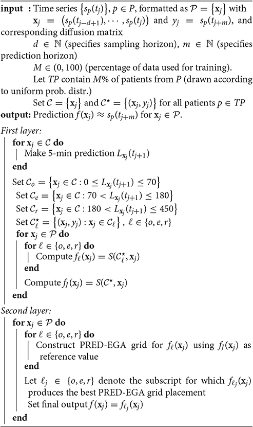
Algorithm 1 Deep Network for BG prediction

FIGURE 1

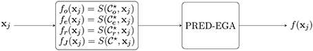
Figure 1. Flowchart diagram: Deep Network for BG prediction.

4.4. Remarks

1. An optional smoothing step may be applied before the first training layer step in Section 4.1 to remove any large spikes in the given time series {s_p(t_j)}, p ∈ P, that may be caused by patient movement, for example. Following ideas in Sparacino et al. [20], we may apply flat low-pass filtering (for example, a first-order Butterworth filter). In this case, the evaluation of the final output in Section 4.3 is done by using the original, unsmoothed measurements as reference values.

2. We remark that, as explained in Section 1, the training set may also be implemented in a different way: instead of drawing M% of the patients in P and using their entire data sets for training, we could construct the training set ${{C}}^{\star }$ for each patient p ∈ P separately by drawing M% of a given patient's data for training, and then construct the networks f_ℓ, ℓ ∈ {o, e, r} and f_J for each patient separately. This is a different problem, studied often in the literature (see for example, [14, 20, 23]). We do not pursue this approach in the current paper.

5. Results and Discussion

As mentioned in Section 2, we apply our method to data provided by the DirecNet Central Laboratory. Time series for 25 patients are considered. This specific data set was designed to study the performance of CGM devices in children with Type I diabetes; as such, all of the patients are less than 18 years old. Each time series {s_p(t_j)} contains more than 160 BG measurements, taken at 5-min intervals. Our method is a general purpose algorithm, where these details do not play any significant role, except in affecting the outcome of the experiments.

We provide results obtained by implementing our method in Matlab, as described in Algorithm 1. For our implementation, we employ a sampling horizon t_j − t_j−d+1 of 30 min (d = 7), a prediction horizon t_j+m − t_j of 30 min (m = 6), and a total of 100 trials (T = 100). We provide results for both 30% training data (M = 30) and 50% training data (M = 50) (which is comparable to approaches followed in for example [13, 14]). After testing our method on all 25 patients, the average PRED-EGA scores (in percent) are displayed in Table 1. For 30% training data, the percentage of accurate predictions and predictions with benign consequences is 84.32% in the hypoglycemic range, 97.63% in the euglycemic range, and 82.89% in the hyperglycemic range, while for 50% training data, we have 93.21% in the hypoglycemic range, 97.68% in the euglycemic range, and 86.78% in the hyperglycemic range.

TABLE 1

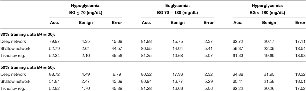
Table 1. Average PRED-EGA scores (in percent): M% of patients used for training.

For comparison, Table 1 also displays the PRED-EGA scores obtained when implementing a shallow (ie, one layer) feed-forward network with 20 neurons using Matlab's Neural Network Toolbox, using the same parameters d, m, M and T as in our implementation, with Matlab's default hyperbolic tangent sigmoid activation function. The motivation for using 20 neurons is the following. As mentioned in Section 4.1, each layer in our deep network can be viewed as a classical neural network with exactly as many neurons as the number of eigenfunctions used in Equations (A9) and (A11). This number is determined to ensure that the system in Equation (A10) is well conditioned; in our experiments, it turned out to be at most 5. Therefore, to compare our two-layer deep network (where the first layer consists of three separate networks) with a classical shallow neural network, we use 20 neurons. It is clear that our deep network performs substantially better than the shallow network; in all three BG ranges, our method produces a lower percentage of erroneous predictions.

For a further comparison, we also display in Table 1 the PRED-EGA scores obtained when training through supervised learning using a standard Tikhonov regularization to find the best least square fit to the data; specifically, we implemented the method described in Poggio and Smale [24, pp. 3–4] using a Gaussian kernel with σ = 100 and regularization constant γ = 0.0001. Again, our method produces superior results, especially in the hypoglycemic range.

Figures 2, 3 display boxplots for the percentage accurate predictions in each BG range for each method over the 100 trials.

FIGURE 2

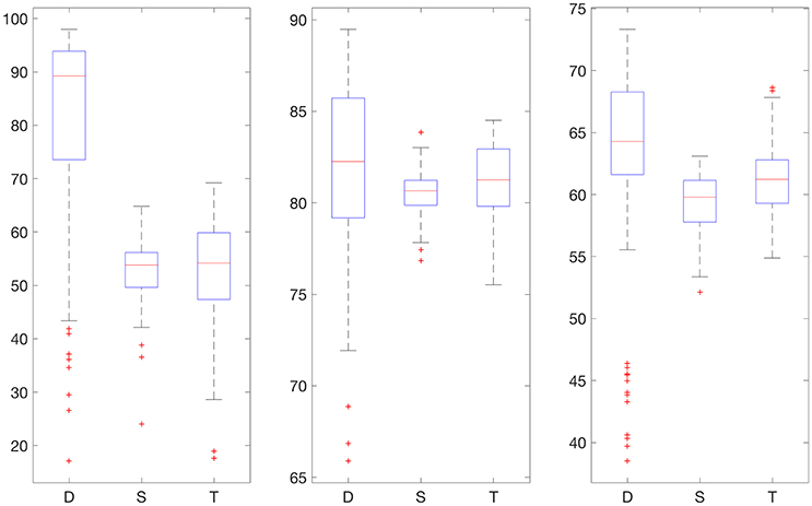
Figure 2. Boxplot for the 100 experiments conducted with no smoothing and 30% training data for each prediction method (D, deep network; S, shallow network; T, Tikhonov regularization). The three graphs show the percentage accurate predictions in the hypoglycemic range (left), euglycemic range (middle), and hyperglycemic range (right).

FIGURE 3

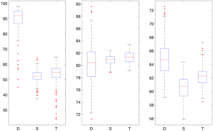
Figure 3. Boxplot for the 100 experiments conducted with no smoothing and 50% training data for each prediction method (D, deep network; S, shallow network; T, Tikhonov regularization). The three graphs show the percentage accurate predictions in the hypoglycemic range (left), euglycemic range (middle) and hyperglycemic range (right).

We also provide results obtained when applying smoothing through flat low-pass filtering to the given time series, as explained in Section 4.4. For our implementations, we used a first-order Butterworth filter with cutoff frequency 0.8, with the same input parameters as before. The results are given in Table 2. For 30% training data, the percentage of accurate predictions and predictions with benign consequences is 88.92% in the hypoglycemic range, 97.64% in the euglycemic range, and 77.58% in the hyperglycemic range, while for 50% training data, we have 96.43% in the hypoglycemic range, 97.96% in the euglycemic range, and 85.29% in the hyperglycemic range. Figures 4, 5 display boxplots for the percentage accurate predictions in each BG range for each method over the 100 trials.

TABLE 2

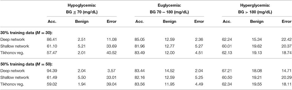
Table 2. Average PRED-EGA scores (in percent): M% of patients used for training with flat low-pass filtering.

FIGURE 4

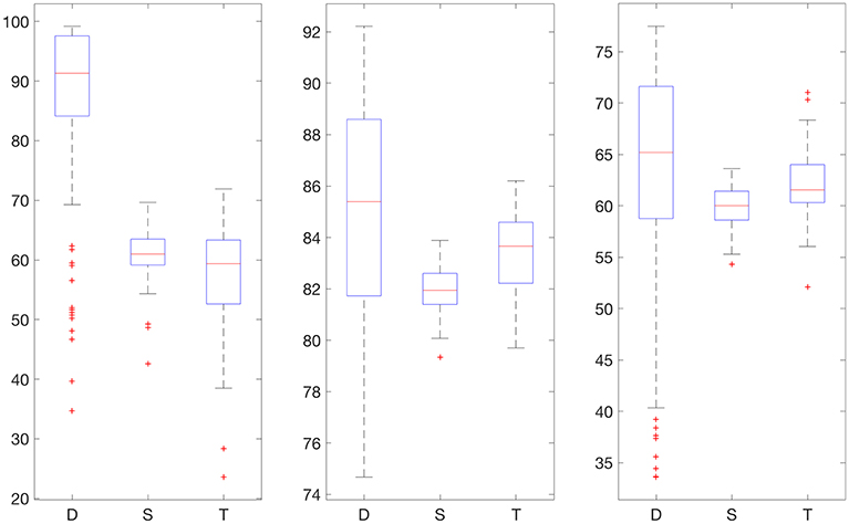
Figure 4. Boxplot for the 100 experiments conducted with flat low-pass filtering and 30% training data for each prediction method (D, deep network; S, shallow network; T, Tikhonov regularization). The three graphs show the percentage accurate predictions in the hypoglycemic range (left), euglycemic range (middle) and hyperglycemic range (right).

FIGURE 5

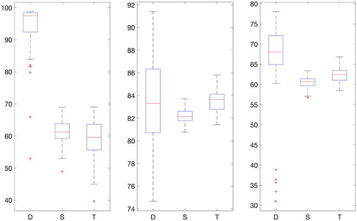
Figure 5. Boxplot for the 100 experiments conducted with flat low-pass filtering and 50% training data for each prediction method (D, deep network; S, shallow network; T, Tikhonov regularization). The three graphs show the percentage accurate predictions in the hypoglycemic range (left), euglycemic range (middle) and hyperglycemic range (right).

In all our experiments the percentage of erroneous predictions is substantially smaller with deep networks than the other two methods we have tried, with the only exception of hyperglycemic range with 30% training data and flat low pass filtering. Our method's performance also improves when the amount of the training data increases from 30% to 50%, because the percentage of erroneous predictions decreases in all of the BG ranges in all experiments.

Moreover, from this viewpoint, our deep learning method outperforms the considered competitors, except in the hyperglycemic BG range in Table 2. A possible explanation for this is that the DirecNet study was done on children (less than 18 years of age) with type 1 diabetes, for a period of roughly 26 h. It appears that children usually have prolonged hypoglycemic periods as well as profound postprandial hyperglycemia (high blood sugar “spikes” after meals)—according to Boland et al. [25], more than 70% of children display prolonged hypoglycemia while more than 90% of children display significant postprandial hyperglycemia. In particular, many of the patients in the data set only exhibit very limited hyperglycemic BG spikes—for the patient labeled 43, for example, there exists a total of 194 BG measurements, of which only 5 measurements are greater than 180 mg/dL. This anomaly might have affected the performance of our algorithm in the hyperglycemic range. Obviously, it performs remarkably better than the other techniques we have tried, including fully supervised training, while ours is only semi-supervised.

6. Conclusion

The prediction of blood glucose levels based on continuous glucose monitoring system data 30 min ahead is a very important problem with many consequences for the health care industry. In this paper, we suggest a deep learning paradigm based on a solid mathematical theory as well as domain knowledge to solve this problem accurately as assessed by the PRED-EGA grid, developed specifically for this purpose. It is demonstrated in Mhaskar and Poggio [4] that deep networks perform substantially better than shallow networks in terms of expressiveness for function approximation when the target function has a compositional structure. Thus, the blessing of compositionality cures the curse of dimensionality. However, the compositional structure is not unique, and it is open problem to decide whether a given target function has a certain compositional structure. In this paper, we have demonstrated an example where domain knowledge can be used to build an appropriate compositional structure, leading to a parsimonious deep learning design.

Ethics Statement

The clinical data set used in this publication is publicly available online [9]. The data were collected during the study that was carried out in accordance with the recommendations of DirecNet, Jaeb Center for Health Research, with written informed consent from all 878 subjects. All subjects gave written informed consent in accordance with the Declaration of Helsinki. The protocol was approved by DirecNet, Jaeb Center for Health Research.

Author Contributions

All authors listed have made a substantial, direct and intellectual contribution to the work, and approved it for publication.

Conflict of Interest Statement

The authors declare that the research was conducted in the absence of any commercial or financial relationships that could be construed as a potential conflict of interest.

Acknowledgments

The research of HM is supported in part by ARO Grant W911NF-15-1-0385. The research of SP is partially supported by Austrian Science Fund (FWF) Grant I 1669-N26.

References

1. Montufar GF, Pascanu R, Cho K, Bengio Y. On the number of linear regions of deep neural networks. In: Advances in Neural Information Processing Systems. Red Hook, NY: Curran Associates, Inc. (2014) p. 2924–32.

Google Scholar

2. Telgarsky M. Representation benefits of deep feedforward networks. arXiv preprint (2015) arXiv:150908101

Google Scholar

3. Safran I, Shamir O. Depth separation in relu networks for approximating smooth non-linear functions. arXiv preprint (2016) arXiv:161009887

Google Scholar

4. Mhaskar HN, Poggio T. Deep vs. shallow networks: an approximation theory perspective. Anal Appl. (2016) 14:829–48. doi: 10.1142/S0219530516400042

CrossRef Full Text | Google Scholar

5. Naumova V, Pereverzyev SV, Sivananthan S. A meta-learning approach to the regularized learning - Case study: blood glucose prediction. Neural Netw. (2012) 33:181–93. doi: 10.1016/j.neunet.2012.05.004

PubMed Abstract | CrossRef Full Text | Google Scholar

6. Snetselaar L. Nutrition Counseling Skills for the Nutrition Care Process. Sudbury, MA: Jones & Bartlett Learning (2009).

Google Scholar

7. Mhaskar HN, Naumova V, Pereverzyev SV. Filtered Legendre expansion method for numerical differentiation at the boundary point with application to blood glucose predictions. Appl Math Comput. (2013) 224:835–47. doi: 10.1016/j.amc.2013.09.015

CrossRef Full Text | Google Scholar

8. Ehler M, Filbir F, Mhaskar HN. Locally learning biomedical data using diffusion frames. J Comput Biol. (2012) 19:1251–64. doi: 10.1089/cmb.2012.0187

PubMed Abstract | CrossRef Full Text | Google Scholar

9. DirecNet Central Laboratory. (2005). Available online at: http://direcnet.jaeb.org/Studies.aspx

10. Hayes AC, Mastrototaro JJ, Moberg SB, Mueller JC Jr, Clark HB, Tolle MCV, et al. Algorithm sensor augmented bolus estimator for semi-closed loop infusion system. Google Patents (2009). US Patent 7,547,281.

Google Scholar

11. Sivananthan S, Naumova V, Man CD, Facchinetti A, Renard E, Cobelli C, et al. Assessment of blood glucose predictors: the prediction-error grid analysis. Diabet Technol Ther. (2011) 13:787–96. doi: 10.1089/dia.2011.0033

PubMed Abstract | CrossRef Full Text | Google Scholar

12. Naumova V, Pereverzyev SV, Sivananthan S. Adaptive parameter choice for one-sided finite difference schemes and its application in diabetes technology. J Complex. (2012) 28:524–38. doi: 10.1016/j.jco.2012.06.001

CrossRef Full Text | Google Scholar

13. Pappada SM, Cameron BD, Rosman PM, Bourey RE, Papadimos TJ, Olorunto W, et al. Neural network-based real-time prediction of glucose in patients with insulin-dependent diabetes. Diabet Technol Ther. (2011) 13:135–41. doi: 10.1089/dia.2010.0104

PubMed Abstract | CrossRef Full Text | Google Scholar

14. Reifman J, Rajaraman S, Gribok A, Ward WK. Predictive monitoring for improved management of glucose levels. J Diabet Sci Technol. (2007) 1:478–86. doi: 10.1177/193229680700100405

PubMed Abstract | CrossRef Full Text | Google Scholar

15. Savitzky A, Golay MJE. Smoothing and differentiation of data by simplified least squares procedures. Anal Chem. (1964) 36:1627–39. doi: 10.1021/ac60214a047

CrossRef Full Text | Google Scholar

16. Lu S, Naumova V, Pereverzev SV. Legendre polynomials as a recommended basis for numerical differentiation in the presence of stochastic white noise. J Inverse ILL Posed Prob. (2013) 21:193–216. doi: 10.1515/jip-2012-0050

CrossRef Full Text | Google Scholar

17. Naumova V, Pereverzyev SV, Sivananthan S. Extrapolation in variable RKHSs with application to the blood glucose reading. Inverse Prob. (2011) 27:075010. doi: 10.1088/0266-5611/27/7/075010

CrossRef Full Text | Google Scholar

18. Pappada SM, Cameron BD, Rosman PM. Development of a neural network for prediction of glucose concentration in type 1 diabetes patients. J Diabet Sci Technol. (2008) 2:792–801. doi: 10.1177/193229680800200507

PubMed Abstract | CrossRef Full Text | Google Scholar

19. Clarke WL, Cox D, Gonder-Frederick LA, Carter W, Pohl SL. Evaluating clinical accuracy of systems for self-monitoring of blood glucose. Diabetes Care (1987) 10:622–8. doi: 10.2337/diacare.10.5.622

PubMed Abstract | CrossRef Full Text | Google Scholar

20. Sparacino G, Zanderigo F, Corazza S, Maran A, Facchinetti A, Cobelli C. Glucose concentration can be predicted ahead in time from continuous glucose monitoring sensor time-series. IEEE Trans Biomed Eng. (2007) 54:931–7. doi: 10.1109/TBME.2006.889774

PubMed Abstract | CrossRef Full Text | Google Scholar

21. Lafon S. Diffusion Maps and Geometric Harmonics. New Haven, CT: Yale University (2004).

Google Scholar

22. Mhaskar HN. Eignets for function approximation on manifolds. Appl Comput Harmon Anal. (2010) 29:63–87. doi: 10.1016/j.acha.2009.08.006

CrossRef Full Text | Google Scholar

23. Eren-Oruklu M, Cinar A, Quinn L, Smith D. Estimation of future glucose concentrations with subject-specific recursive linear models. Diabet Technol Ther. (2009) 11:243–53. doi: 10.1089/dia.2008.0065

PubMed Abstract | CrossRef Full Text | Google Scholar

24. Poggio T, Smale S. The mathematics of learning: dealing with data. Notices AMS (2003) 50:537–44. Available online at: http://www.ams.org/notices/200305/fea-smale.pdf

Google Scholar

25. Boland E, Monsod T, Delucia M, Brandt CA, Fernando S, Tamborlane WV. Limitations of conventional methods of self-monitoring of blood glucose lessons learned from 3 days of continuous glucose sensing in pediatric patients with type 1 diabetes. Diabetes Care (2001) 24:1858–62. doi: 10.2337/diacare.24.11.1858

PubMed Abstract | CrossRef Full Text | Google Scholar

26. Maggioni M, Mhaskar HN. Diffusion polynomial frames on metric measure spaces. Appl Comput Harmon Anal. (2008) 24:329–53. doi: 10.1016/j.acha.2007.07.001

CrossRef Full Text | Google Scholar

27. Belkin M, Niyogi P. Towards a theoretical foundation for Laplacian-based manifold methods. In: International Conference on Computational Learning Theory. Berlin: Springer (2005). p. 486–500. doi: 10.1007/11503415_33

CrossRef Full Text | Google Scholar

28. Singer A. From graph to manifold Laplacian: the convergence rate. Appl Comput Harmon Anal. (2006) 21:128–34. doi: 10.1016/j.acha.2006.03.004

CrossRef Full Text | Google Scholar

A. Appendix

A.1. Filtered Legendre Expansion Method

In this appendix, we review the mathematical background for the method developed in Mhaskar et al. [7] for short term blood glucose prediction. As explained in the text, the main mathematical problem can be summarized as that of estimating the derivative of a function at the end point of an interval, based on measurements of the function in the past. Mathematically, if f : [−1, 1] → ℝ is continuously differentiable, we wish to estimate f′(1) given the noisy values {y_j = f(t_j) + ϵ_j} at points ${\left\{t_j\right\}}_{j=1}^d\subset \left[-1,1\right]$. We summarize only the method here, and refer the reader to Mhaskar et al. [7] for the detailed proof of the mathematical facts.

For this purpose, we define the Legendre polynomials recursively by

$\begin{array}{l}{P}_k(x)=\frac{2k-1}{2k}x{P}_{k-1}(x)-\frac{k-1}{k}{P}_{k-2}(x),k=2,3,\dots ;\\ P_0(x)=1,P_1(x)=x.\end{array}$

Let h:ℝ → ℝ be an even, infinitely differentiable function, such that h(t) = 1 if t ∈ [0, 1/2] and h(t) = 0 if t ≥ 1. We define

$K_n(h;x)=\frac{1}{2}{\displaystyle \sum _{k=0}^{n-1}h}\left(\frac{k}{n}\right)k(k+1/2)(k+1)P_k(x).$

Next, given the points ${\left\{t_j\right\}}_{j=1}^d\subset \left[-1,1\right]$, we use least squares to find n = n_d such that

${\displaystyle \sum _{j=1}^n{w}_j}{P}_k(t_j)={\displaystyle {\int }_{-1}^1{P}_k}(t)dt=\{\begin{array}{ll}2,\hfill & \text{if }k=0,\hfill \\ 0,\hfill & \text{if }1\le k<2n,\hfill & (\text{A}1)\end{array}$

and the following estimates are valid for all polynomials of degree < 2n:

${\displaystyle \sum _{j=1}^n|}{w}_{j}P(t_j)|\le A{\displaystyle {\int }_{-1}^1|}P(t)|dt,$

for some positive constant A. We do not need to determine A, but it is guaranteed to be proportional to the condition number of the system in Equation (A1).

Finally, our estimate of f′(1) based on the values y_j = f(t_j)+ϵ_j, j = 1, ⋯ , d, is given by

${{S}}_n(h;\{y_j\})={\displaystyle \sum _{j=1}^d{w}_j}{y}_j{K}_n(h;t_j).$

It is proved in Mhaskar et al. [7, Theorem 3.2] that if f is twice continuously differentiable,

${\Delta }_{[-1,1]}(f)(x)=2x{f}^{\prime }(x)-(1-x^2)f^{″}(x),$

and |ϵ_j| ≤ δ then

$|{{S}}_n(h;\{y_j\})-f^{\prime }(1)|\le cA\left\{E_{n/2,[-1,1]}({\Delta }_{[-1,1]}(f))+n^2\delta \right\},$

where

$E_{n/2,[-1,1]}({\Delta }_{[-1,1]}(f))=\min \underset{x\in [-1,1]}{\max }|{\Delta }_{[-1,1]}(f)(x)-P(x)|,(\text{A}2)$

the minimum being over all polynomials P of degree < n/2.

A.2. Function Approximation on Data Defined Spaces

While classical approximation theory literature deals with function approximation based on data that is dense on a known domain, such as a cube, torus, sphere, etc., this condition is generally not satisfied in the context of machine learning. For example, the set of vectors (s_p(t_j), …, s_p(t_j − d + 1)) is unlikely to be dense in a cube in ℝ^d. A relatively recent idea is to think of the data as being sampled from a distribution on an unknown manifold, or more generally, a locally compact, quasi-metric measure space. In this appendix, we review the theoretical background that underlies our experiments reported in this paper. The discussion here is based mainly on Maggioni and Mhaskar [26], Mhaskar [22], and Ehler et al. [8].

Let 𝕏 be a locally compact quasi-metric measure space, with ρ being the quasi-metric and μ* being the measure. In the context of machine learning, μ* is a probability measure and 𝕏 is its support. The starting point of this theory is a non-decreasing sequence of numbers ${\left\{{\lambda }_k\right\}}_{k=0}^{\infty }$, such that λ₀ = 0 and λ_k → ∞ as k → ∞, and a corresponding sequence of bounded functions ${\left\{{\varphi }_k\right\}}_{k=0}^{\infty }$ that forms an orthonormal sequence in L²(μ*). Let Π_λ = span{ϕ_k : λ_k < λ}, and analogously to Equation (A2), we define for a uniformly continuous, bounded function f : 𝕏 → ℝ,

$E_{\lambda }(f)=\underset{P\in {\Pi }_{\lambda }}{\min }\underset{x\in 𝕏}{\sup }|f(x)-P(x)|.$

With the function h as defined in Appendix A.1, we define

${\Phi }_{\lambda }(h;x,y)={\displaystyle \sum _{k:{\lambda }_k<\lambda }h}\left(\frac{{\lambda }_k}{\lambda }\right){\varphi }_k(x){\varphi }_k(y),x,y\in 𝕏.(\text{A}3)$

Next, let ${\left\{x_j\right\}}_{j=1}^M\subset 𝕏$ be the “training data”. Our goal is to learn a function f : 𝕏 → ℝ based on the values ${\left\{f(x_j)\right\}}_{j=1}^M$. Toward this goal, we solve an under-determined system of equations

${\displaystyle \sum _{j=1}^M{W}_j}{\varphi }_k(x_j)=\{\begin{array}{ll}1,\hfill & \text{if }k=0,\hfill \\ 0,\hfill & \text{if }k>0,\hfill \end{array}k:{\lambda }_k<\lambda (\text{A}4)$

for the largest possible λ for which this system is still well conditioned. We then define an approximation, analogous to the classical radial basis function networks, by

${\sigma }_{\lambda }(h;f,x)={\displaystyle \sum _{j=1}^M{W}_j}f(x_j){\Phi }_{\lambda }(x,x_j),x\in 𝕏.(\text{A}5)$

It is proved in Maggioni and Mhaskar [26], Mhaskar [22], and Ehler et al. [8] that under certain technical conditions, for a uniformly continuous, bounded function f : 𝕏 → ℝ, we have

$E_{\lambda }(f)\le \underset{x\in 𝕏}{\sup }|f(x)-{\sigma }_{\lambda }(h;f,x)|\le c{E}_{\lambda /2}(f),$

where c > 0 is a generic positive constant. Thus, the approximation σ_λ(f) is guaranteed to yield a “good approximation” that is asymptotically best possible given the training data.

In practice, one has a point cloud ${P}={\left\{y_i\right\}}_{i=1}^N\supset {\left\{x_j\right\}}_{j=1}^M$ rather than the space 𝕏. The set ${P}$ is a subset of some Euclidean space ℝ^D for a possibly high value of D, but is assumed to lie on a compact sub-manifold 𝕏 of ℝ^D, with this manifold having a low dimension. We build the graph Laplacian from ${P}$ as follows: With a parameter ε > 0, induces the weight matrix ${{W}}_N^{\epsilon }$ defined by

${{W}}_{N;i,j}^{\epsilon }=\exp (-|y_i-y_j{|}^2/\epsilon ).(\text{A}6)$

We build the diagonal matrix $D_{N;i,i}^{\epsilon }=\sum _{j=1}^N{{W}}_{N;i,j}^{\epsilon }$ and define the (unnormalized) graph Laplacian as

$L_N^{\epsilon }={{W}}_N^{\epsilon }-D_N^{\epsilon }.$

Various other versions of this Laplacian are also used in practice. For M → ∞ and ε → 0, the eigenvalues and interpolations of the eigenvectors of $L_M^{\epsilon }$ converge toward the “interesting” eigenvalues λ_k and eigenfunctions ϕ_k of a differential operator Δ_𝕏. This behavior has been studied in detail by many authors, e.g., Belkin and Niyogi [27], Lafon [21], and Singer [28]. When ${\left\{y_i\right\}}_{i=1}^M$ are uniformly distributed on 𝕏, this operator is the Laplace-Beltrami operator on 𝕏. If ${\left\{y_i\right\}}_{i=1}^M$ are distributed according to the density p, then the graph Laplacian approximates the elliptic Schrödinger type operator $\Delta +\frac{\Delta p}{p}$, whose eigenfunctions ϕ_k also form an orthonormal basis for L₂(𝕏, μ).