Better Autologistic Regression

1. Introduction

The autologistic (AL) model is a probabilistic graphical model for multivariate binary data. It was introduced to the statistical literature by Besag [1, 2] and has also been developed by Kaiser and Cressie [3]. The same model appeared much earlier in statistical physics, where it is known as the Ising model (see e.g., [4, 5]). It has been used extensively in image processing (e.g., [6–8]), and is also the model underlying the Boltzmann machine [9]. The same model has also been called the quadratic exponential binary distribution [10, 11], and, under that name, it has been described as the binary-variable analog of the multivariate normal distribution ([12]; see also [13]). As such, one may anticipate that the autologistic model will become increasingly useful as the number of complex, graph-structured data sets continues to grow.

When binary responses are observed along with covariate information, the autologistic model may be extended to become the autologistic regression (ALR) model. This model can be viewed as a natural extension of ordinary logistic regression to handle cases where responses are not independent. Under the ALR model, the responses follow an autologistic distribution, and the distribution's parameters are written in terms of a linear predictor involving the covariates. The ALR model has been used in a variety of fields, including ecology [14, 15], dentistry [16, 17], anthropology [18], materials science [19] and computer vision [20, 21].

As an example, consider the Hydrocotyle vulgaris data shown in Figure 1. These data were derived from the work of Carl and Kühn [22] and re-analyzed by Bardos et al. [23]. The responses are presence or absence of plant species H. vulgaris in a regular grid of 2,995 cells covering Germany. The covariate is altitude (in hundreds of meters), recorded as a number from 0 to 18.23. From the figure it is clear that altitude is inversely related to species presence, and also that the observed responses are spatially correlated. Simple logistic regression provides estimated probabilities that appear realistic, but samples drawn from the fitted logistic model have more noise than the observed response. Explicitly modeling spatial association through an ALR model can potentially improve goodness-of-fit and give a better evaluation of the true effect of altitude.

FIGURE 1

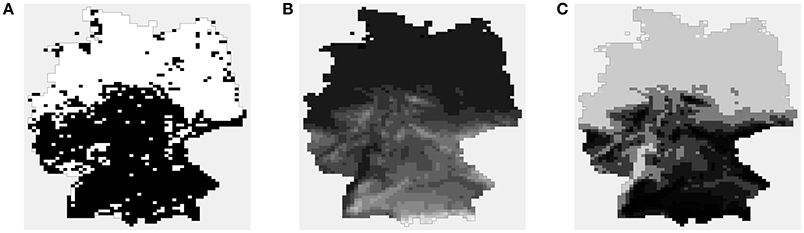
Figure 1. The H. vulgaris data. (A) Observed presence/absence data (white indicates presence, which is taken to be the “high” level). (B) Value of the covariate, altitude. (C) Predicted probabilities from logistic regression. In (B,C), lighter shades of gray indicate larger values.

If an analyst wishes to perform autologistic regression on data such as these, they are faced with two choices about the structure of the model: coding and centering.

Coding refers to the pair of numbers used to represent the two possible states or levels of a binary variable. Here the two levels will be referred to as “low” and “high.” Since binary outcomes are usually categorical, not numeric, the analyst may freely choose two values, ℓ and h, to represent the two states. Standard choices are the zero/one coding, {0, 1}, used almost universally in the statistics literature, and the plus/minus coding, {−1, 1}, used customarily in physics and also common in image processing.

Centering refers to the presence or absence of a particular term in the model formulae. Caragea and Kaiser [24] observed that the original ALR model provides regression coefficient estimates that are not easy to interpret. They proposed the centered model to correct this problem, and recommended that it become the default for future use. This viewpoint was furthered by Hughes et al. [25], who expanded on inferential and computational aspects of ALR, using the centered model exclusively.

One may, then, refer to two types of AL/ALR model: those with the centering adjustment (centered models), and those without it (standard models). Additionally, each type may be used with any chosen coding, leading to an infinite number of model variants (a term that will be used for a particular combination of type and coding).

The present work provides a detailed study of the different AL and ALR variants. It is confirmed that all variants are equivalent in the AL case, although the way they depend on their parameters varies widely. More interestingly, equivalence does not hold in the ALR case. The centered and standard ALR models are distinct, non-nested families of probability distributions. Even within ALR models of the same type, changing the coding will generally change its probabilistic structure. The differences among models can be large both qualitatively and quantitatively, certainly large enough to be of practical consequence.

The extant literature on autologistic regression does not contain a similar investigation of the impact of coding and centering. Indeed, it appears to demonstrate ambiguity about the importance of these two choices. Consider the following:

1. Some research communities use {0, 1} coding, and others use {−1, 1}. At the same time, the author is not aware of a single article in which a justification was given for choosing one coding over the other in an ALR model.

2. In the literature, ALR models with different codings take the same algebraic form; a coding change is effected by simply plugging different numbers into the same formulae. This is done despite the well-known fact (repeated in Appendix A) that this operation is not, in general, equivalent to properly transforming the random variables.

3. The key references for the centered model [24, 25] both refer to it as an autologistic model with a “centered parameterization,” and cite improved parameter interpretation as its main advantage.

4. The centering adjustment was motivated by analogy with Gaussian models, where both centered and uncentered models are part of the same distribution family.

Points 1 and 2 suggest that many researchers view the choice of coding in an ALR model as trivial or inconsequential. This misconception might arise because the coding change is a seemingly innocuous linear transformation of the responses, one which is trivial in the AL model. Points 3 and 4 show how a reader might come to assume that centered and standard ALR models are equivalent to one another, differing only by a parameter transformation.

The current work resolves the above misconceptions, and should help analysts develop better autologistic regression models by understanding the consequences of their modeling choices.

Throughout this research, one group of equivalent variants was repeatedly found to have unique and attractive properties. It is the set of standard models with coding that sums to zero, like {−h, h}. This model will be referred to as the symmetric autologistic model. It resolves the problems with the standard zero/one-coded model in a manner that is simpler and more natural than the centered model, and it is conceptually more appealing as a generative model for binary data.

The results are developed as follows. Section 2 provides more detail on the AL and ALR models, in both standard and centered forms. It also gives a general form of the model that includes both model types under arbitrary coding. The general form is used in section 3 to establish several theoretical results, including results about model equivalence and behavior in the limit as the inter-variable association increases. Section 4 provides numerical examples that demonstrate the differences among the model variants, while also illustrating and corroborating the theory. The H. vulgaris data is also analyzed at the end of section 4. Section 5 summarizes the results and provides further discussion about the symmetric model.

2. Autologistic Models

This section lays out details of the AL and ALR models under different coding and centering choices. Because the notation and terminology used to describe these models varies considerably across disciplines, it is not assumed that every reader is familiar with the way the models are developed here. A somewhat expository tone is taken in this section.

2.1. Markov Random Fields

The AL model is best understood as a Markov random field (MRF) of binary random variables. MRFs provide a general framework for modeling collections of random variables, where the dependence among the variables is encoded by an undirected graph. We are interested in the binary case.

Let $\text{Z}={\left[Z_1,Z_2,\dots ,Z_n\right]}^T$ be a vector of n dichotomous random variables (with coding as yet unspecified). Associated with Z is a graph ${G}=({V},{E})$ having vertices ${V}=\left\{1,2,\dots ,n\right\}$ (also called nodes; one for each variable) and edges ${E}=\left\{(i,j):i<j,i~j\right\}$, where i, j ∈ {1, 2, …, n}, and i ~ j means variables i and j share an edge. Variables that are joined by an edge are called neighbors of one another.

The role of the graph is to define conditional independence statements. Specifically, let Z_−i represent all of the variables except for the ith, and let Z_j~i represent all of the neighbors of Z_i in the graph. In an MRF, each variable is conditionally independent of the others, given its neighbors: Pr(Z_i = z_i|Z_−i) = Pr(Z_i = z_i|Z_j~i).

The joint distribution of an MRF can be expressed as a Boltzmann (or Gibbs) distribution:

$\begin{array}{ll}f(\text{z})=\frac{1}{c}{e}^{Q(\text{z})},& (1)\end{array}$

where Q(z) is called the negpotential function and the normalizing constant c is known as the partition function. It is also common for Q(z) to be referred to as an energy function, in which case it is usually preceded by a negative sign, and sometimes divided by a temperature parameter.

The negpotential function for any MRF can be expressed as a sum of functions of cliques of variables (that is, groups of fully connected vertices in the graph). Letting ${M}$ represent the set of cliques, we have

$\begin{array}{ll}Q(\text{z})={\displaystyle \sum _{m\in {M}}}{\psi }_m({\text{z}}_m).& (2)\end{array}$

The sum consists of one function per clique, with the mth function depending only on the variables that are part of the mth clique. This fundamental result is known as the Hammersley-Clifford theorem; see Besag [2, 26] and Kaiser and Cressie [3] for more details and technical conditions on this MRF-Gibbs equivalence.

The high degree of generality of Equations (1) and (2) makes MRFs attractive for modeling complex associations. The graph structure determines which variables appear together in the ψ_m functions, and the the functions themselves can be specified to control which arrangements of variables get greater probability mass. The price paid for this flexibility is computational: for most practical problems the partition function can not be computed in reasonable time.

We will subsequently focus on the particular form of the negpotential function used in the autologistic model. Our development of the AL model is consistent with that given in Hughes et al. [25], which also gives an excellent review of the computational aspects of inference with the AL model. For more on MRFs and graphical models in general, see e.g., [27–30].

2.2. Standard and Centered Models with Zero/One Coding

Both the standard and centered models have been developed under the assumption of {0, 1} coding. This section describes these models under the same assumption.

The autologistic model is a member of the class of so-called pairwise MRFs, where only cliques of size one or two have nonzero contribution to the negpotential function. The standard model has negpotential function

$\begin{array}{ll}{Q}_{\text{std}}(\text{z})={\displaystyle \sum _{i\in {V}}}{\alpha }_i{z}_i+{\displaystyle \sum _{(i,j)\in {E}}}{\lambda }_{ij}{z}_i{z}_j.& (3)\end{array}$

The right hand side of Equation (3) contains two sums. The first is over all vertices in the graph, and includes each individual variable's contributions to the probability mass function (PMF). The second is over all edges in the graph, and includes the contribution of each pair of neighbor variables. Values {α_i} and {λ_ij} are called the unary and pairwise parameters, respectively. Note that if λ_ij = 0, ∀i, j, the PMF factorizes and Z₁, …, Z_n are mutually independent.

The MRF-Gibbs equivalence makes it possible to specify the AL model through its conditional distributions. The conditional distributions are also used to write the conditional logit form of the model. Let ${\pi }_i^{*}=Pr(Z_i=1|{\text{Z}}_{-i})$. Then it can be shown that the standard model has conditional log odds

$\begin{array}{ll}\text{logit}({\pi }_i^{*})=log\left(\frac{{\pi }_i^{*}}{1-{\pi }_i^{*}}\right)={\alpha }_i+{\displaystyle \sum _{j~i}}{\lambda }_{ij}{z}_j,& (4)\end{array}$

where $\sum _{j~i}$ denotes the sum over all j that are neighbors of i. The log odds depends on the ith variable's unary parameter plus a weighted sum of its neighbors' values. Increasing α_i or having more neighbors that take value 1 will increase the odds of observing a 1 in location i.

Inspection of Equation (4) hints at the parameter interpretation problem noted in Caragea and Kaiser [24]. The influence of the neighbor states on the conditional logit is asymmetric. Any neighbors taking value 0 contribute nothing to the conditional log odds, while neighbors with value 1 increase the log odds. No configuration of neighbors can cause $\text{logit}({\pi }_i^{*})$ to decrease below the value of α_i. This effectively couples the unary and pairwise parameters' effects.

The centered autologistic model was proposed as a modified form to ameliorate this problem. The centered model has conditional logit form

$\begin{array}{ll}\text{logit}({\pi }_i^{*})={\alpha }_i+{\displaystyle \sum _{j~i}}{\lambda }_{ij}(z_j-{\mu }_j^{*}),& (5)\end{array}$

where the centering adjustment, ${\mu }_j^{*}$, is the expectation of the jth variable under the assumption of independence:

$\begin{array}{ll}{\mu }_j^{*}=\text{ E}[Z_j|{\lambda }_{ij}=0,\forall i,j]=\frac{e^{{\alpha }_j}}{1+e^{{\alpha }_j}}.& (6)\end{array}$

2.3. A General Form

We now drop the requirement of {0,1} coding, and express the autologistic model in a way that uses arbitrary coding and includes both centered and standard types as special cases. This may be done by defining the conditional distributions in a coding-agnostic manner, and then deriving the joint mass function using the MRF formalism. If the derivation is done for the centered case, any desired autologistic variant can be obtained afterwards by fixing the coding and either retaining the centering adjustment or setting it to zero. Details of the derivation are given in Appendix B, with only the results shown here.

Let the low and high values of the coding be ℓ and h, respectively (with ℓ < h). First consider the centering adjustment for the jth variable, which is denoted by μ_j in this general setting. For standard models, μ_j = 0. For centered models, μ_j is the mean of Z_j under the assumption of independence:

$\begin{array}{l}{\mu }_j=E[Z_j|{\lambda }_{ij}=0,\forall i,j]\\ =\ell Pr(Z_j=\ell |\forall {\lambda }_{ij}=0)+hPr(Z_j=h|\forall {\lambda }_{ij}=0)\\ =\frac{\ell e^{\ell {\alpha }_j}+h{e}^{h{\alpha }_j}}{e^{\ell {\alpha }_j}+e^{h{\alpha }_j}}.& (7)\end{array}$

The conditional forms of the model involve a term that is a sum of neighbor contributions. To simplify notation, define this neighbor sum for the ith variable to be

$\begin{array}{ll}{s}_i={\displaystyle \sum _{j~i}}{\lambda }_{ij}(z_j-{\mu }_j).& (8)\end{array}$

Then the conditional PMF of Z_i, given all other Z values, is

$\begin{array}{ll}Pr(Z_i=z_i|{\text{Z}}_{-i})=\frac{\text{exp}(z_i({\alpha }_i+s_i))}{\text{exp}(\ell ({\alpha }_i+s_i))+\text{exp}(h({\alpha }_i+s_i))}& (9)\end{array}$

and, letting π_i = Pr(Z_i = h|Z_−i), the log odds form of the model is

$\begin{array}{ll}\text{logit}({\pi }_i)=(h-\ell )({\alpha }_i+s_i).& (10)\end{array}$

Note that Equations (5) and (6) are special cases of Equations (10) and (7), with ℓ = 0 and h = 1.

Finally, the joint PMF can be derived from the conditional form. To minimize ambiguity, it is included as a definition.

DEFINITION 1 (autologistic model). Let Z be a vector of n dichotomous random variables with low and high values coded ℓ and h, respectively. Under the autologistic model, Z has PMF

$\begin{array}{ll}{f}_{\text{Z}}(\text{z};\alpha ,\Lambda )\propto \text{exp}({\text{z}}^T\alpha -{\text{z}}^T\Lambda {\mu }_{\alpha }+\frac{1}{2}{\text{z}}^T\Lambda \text{z}),& (11)\end{array}$

where Λ is an n × n symmetric matrix with (i, j)th and (j, i)th elements equal to λ_ij if i ~ j, and equal to zero otherwise; and

$\begin{array}{ll}{\mu }_{\alpha }=\{\begin{array}{cc}0& forastandardmodel\\ {[{\mu }_1^{\alpha }\cdots {\mu }_n^{\alpha }]}^T& \text{with }{\mu }_j^{\alpha }=\frac{\ell e^{\ell {\alpha }_j}+h{e}^{h{\alpha }_j}}{e^{\ell {\alpha }_j}+e^{h{\alpha }_j}}foracenteredmodel\end{array}.& (12)\end{array}$

Call coefficient $\alpha ={[{\alpha }_1,\dots ,{\alpha }_n]}^T$ the unary parameter, and call Λ the association matrix. As a compact notation, refer to the standard model as S_ℓ,h(α, Λ) and to the centered model as C_ℓ,h(α, Λ).

This definition gives the negpotential function in matrix-vector form. The association matrix Λ has the same pattern of nonzero elements as the adjacency matrix, A, of the graph. It is common in applications to assume that the association parameter takes a constant value λ throughout the graph, in which case Λ = λA. This will be called the simple smoothing assumption.

Equation (11) looks the same as the (zero/one coded, centered) PMF in Hughes et al. [25], but note that in the present case the centering term is a function of not only the unary parameter, but of ℓ and h as well. The vector of centering adjustments, μ_α, has been written with a subscript as a reminder of its dependence on α.

Equations (9), (10), and (11) express the model in different ways. To reiterate, the standard model is obtained by setting μ = 0, and any desired coding can be obtained by setting {ℓ, h} accordingly.

2.4. Autologistic Regression

The AL model just presented does not include covariate effects. The usual way to introduce covariates is to replace the unary parameters by linear predictors. This is formalized in a definition.

DEFINITION 2 (autologistic regression model). Let Z and f_Z be the same as in Definition 1. Let X be an n × p matrix of covariate information (including intercept if desired), with p < n. Define ${\text{x}}_i^T$ to be the ith row of X, and let β be a p-vector of coefficients. Then the autologistic regression model for Z is f_Z(z; Xβ, Λ). In other words, it is model (11) with ${\alpha }_i\equiv {\text{x}}_i^T\beta$.

The ALR model replaces the n unary parameters {α_i} by the p regression coefficients β. The covariates appear only in the unary parameter, as part of the linear relationship α = Xβ. Once the linear predictor values are fixed, the ALR model becomes an AL model. Because of this, the qualitative behavior of an ALR model is the same as that of an AL model, and if we understand how to interpret α, the interpretation of β will be the same. For this reason the results and analyses of sections 3 and 4 are based primarily on the AL model, unless they specifically relate to the regression parameters.

2.5. About the Parameters

Regardless of centering or coding choice, the graphical nature of the AL/ALR model and its mathematical form both strongly suggest a certain parameter interpretation. The unary parameters control each variable's inherent tendency to take one value or the other. All else being equal, large positive values of α_i (or ${\text{x}}_i^T\beta$) should indicate a high chance to observe the h state at location i, and large negative values should indicate a high chance of ℓ. The pairwise parameters control the amount of influence neighbor variables have on each other, and therefore control the association structure. Following Towner et al. [18], call an edge concordant if the two vertices it joins both take the same state, and discordant if they differ. Large positive λ_ij values should increase the chance that the edge joining Z_i and Z_j is concordant. Negative λ_ij values promote discordant edges. It is assumed throughout this work that all λ_ij ≥ 0, since positive association is of greater practical interest.

All variants of the model share the property that λ_ij = 0, ∀i, j corresponds to statistical independence. The model's behavior under independence will be called its endogenous structure, and the probability that variable i takes its high value, under independence, will be called its endogenous probability, p_i. Other authors [24, 25], in the context of spatial data with smoothly-varying covariates, have used the term “large scale” structure to refer to the model's predictions under independence. “Endogenous” has been preferred here because the graph need not be spatially referenced, nor do the unary parameter values need to be locally smooth.

The explicit goal of the centered ALR model [24, p. 286] was to make the marginal probabilities remain close to the endogenous probabilities even when λ is nonzero, so that the regression coefficients can be said to control the marginal probabilities regardless of association level. Marginal structure is only part of the story, however: the model describes a distribution over the 2ⁿ possible outcomes in its sample space. Each outcome corresponds to a configuration, which is the arrangement of high and low states, irrespective of their numerical coding.

DEFINITION 3 (configuration). The term configuration may be used to refer to either a) any particular outcome in the sample space of a dichotomous random vector, or b) the locations of an outcome's high- and low-valued elements. Two binary vectors with different coding represent the same configuration if the locations of their high- and low-valued elements coincide.

If we repeatedly sample from an AL model with a nonzero association matrix, the configurations that we observe will be the result of a trade-off between the endogenous part of the model (which depends on α alone) and the association effects (depending on Λ) propagating through the graph. It is crucial, then, to understand how the distribution of configurations changes to reflect this trade-off as the association is increased from zero. This understanding is necessary for proper parameter interpretation, and also for assessing the model as a reasonable data-generating process to approximate real-world phenomena.

3. Theoretical Results

This section provides theorems that help to discern the differences among the AL/ALR model variants. The first results consider whether or not different variants are equivalent to each other. Subsequent theorems address the behavior of the different variants in the limit as the association parameter grows large. The section closes with a result on convexity of the pseudolikelihood function.

3.1. Equivalence of AL Models

There is potential for confusion when comparing two models that may differ in both their variable coding and their parametrization. To minimize this, model equivalence is first defined in a coding-independent way.

DEFINITION 4 (equivalent models). Let f₁(z; θ₁) and f₂(y; θ₂) be two joint PMFs for n binary outcomes, where z and y need not have the same coding. Model f₁ is equivalent to model f₂ if, for any θ₂, there exists a ${\theta }_1^{*}$ such that $f_1(\text{z};{\theta }_1^{*})=f_2(\text{y};{\theta }_2)$ whenever z and y represent the same configuration.

Equivalence means that given f₂ with fixed θ₂, there is always a parameter setting of f₁ that makes the two models assign the same probability distribution over the 2ⁿ configurations. The following theorem shows that all variants of the autologistic model are equivalent to the standard model. It only applies to AL models, not to ALR models.

THEOREM 1 (equivalence of AL models). Let f(·;ϕ, Ω) be an autologistic model (either centered or standard), with variable coding {L, H}. Then f is equivalent to S_ℓ,h(α, Λ), a standard model with coding {ℓ, h}. Furthermore, the parameter transformation that makes it equivalent is

$\begin{array}{ll}\alpha =a(\varphi -\Omega {\mu }_{\varphi }+b\Omega \text{1})& (13)\end{array}$

$\begin{array}{ll}\Lambda =a^2\Omega ,& (14)\end{array}$

where $a=\frac{H-L}{h-\ell }$, b = L − aℓ, and 1 is a vector of ones.

PROOF: Let Y be a vector of binary random variables coded {L, H}, and let f_Y(y; ϕ, Ω) be an autologistic model of either type. Let Z be a vector of binary random variables of the same dimension as Y, coded {ℓ, h} and having standard autologistic PMF f_Z = S_ℓ,h(α, Λ). Equivalence requires that f_Y(y) = f_Z(z) whenever y and z represent the same configuration. But in that case, there is a one-to-one transformation linking the two vectors: y = az + b1, with a and b as in the theorem. We have equivalence, then, if we can choose α and Λ such that f_Z(z; α, Λ) = f_Y(az + b1; ϕ, Ω) for all z.

From Equation (11), the negpotential function for the standard model f_Z(z) is

$\begin{array}{ll}{Q}_{\text{Z}}(\text{z};\alpha ,\Lambda )={\text{z}}^T\alpha +\frac{1}{2}{\text{z}}^T\Lambda \text{z}.& (15)\end{array}$

For f_Y(az + b1), which could be of either centered or standard type, the negpotential function is

$\begin{array}{l}{Q}_{\text{Y}}(a\text{z}+b\text{1};\varphi ,\Omega )={(a\text{z}+b\text{1})}^T(\varphi -\Omega {\mu }_{\varphi })\\ +\frac{1}{2}{(a\text{z}+b\text{1})}^T\Omega (a\text{z}+b\text{1})\\ =a{\text{z}}^T(\varphi -\Omega {\mu }_{\varphi }+b\Omega \text{1})\\ +\frac{1}{2}{a}^2{\text{z}}^T\Omega \text{z}+w,& (16)\end{array}$

where the last line was obtained by multiplying out the products and moving terms free of z into the constant w.

The two PMFs are specified only up to a proportionality constant, so equivalence of the PMFs holds if and only if exp(Q_Z(z; α, Λ)) and exp(Q_Y(az + b1; ϕ, Ω) can be made proportional to each other—or alternatively, if the two negpotential functions can be made to differ by at most a z-free additive constant. For the difference of the right-hand sides of Equations (15) and (16) to be z-free, we must have

$\begin{array}{l}{\text{z}}^T\left[\alpha -a(\varphi -\Omega {\mu }_{\varphi }+b\Omega \text{1})\right]+\frac{1}{2}{\text{z}}^T(\Lambda -a^2\Omega )\text{z}=0.\end{array}$

Since this must hold for all z, the coefficients of both the linear and quadratic terms must be zero, which leads us to the transformation given in the theorem. The existence of the transformation proves that the models are equivalent, and because the result does not depend on the particular form of μ_ϕ, it holds regardless of whether f_Y is a centered or standard model. □

If f in Theorem 1 is a standard autologistic model, μ_ϕ = 0 and Equation (13) may be solved explicitly for either α or ϕ. This shows that there is a one-to-one correspondence between standard models with different codings. When f is a centered model, however, Equation (13) is a system of nonlinear equations in ϕ, and since the inverse transformation can not be analytically determined, it remains unclear if the mapping between α and ϕ is one-to-one. The implicit function theorem of vector calculus [31, section 12.8] could be used to show that the inverse exists for all α, but it is not straightforward to show that the Jacobian determinant of transformation (13) is always nonzero. Consequently, Theorem 1 only shows that every autologistic model is equivalent to any chosen model of standard type; it falls short of claiming full one-to-one correspondence between all AL model variants. Nevertheless, it may be conjectured that such a correspondence does exist, and system (13) has been successfully solved for ϕ numerically, using a fixed-point iteration scheme.

3.2. Non-equivalence of ALR Models

The next theorem implies that the equivalence observed among the autologistic models does not, in general, carry over to autologistic regression models.

THEOREM 2 (condition for equivalence of ALR models). Let X be an n×p matrix with n > p, and let f₁(·;Xγ, Ω) and f₂(·;Xβ, Λ) be two autologistic regression models, using coding {L, H} and {ℓ, h}, respectively. Then model f₂ is equivalent to f₁ if and only if β satisfies

$\begin{array}{ll}\text{X}\beta -a^2\Omega {\mu }_{\text{X}\beta }=a\text{X}\gamma +a\Omega (b\text{1}-{\mu }_{\text{X}\gamma }),& (17)\end{array}$

where a and b are as defined in Theorem 1. This is an overdetermined system of equations in β (linear equations if f₂ is a standard model, and nonlinear if it is centered).

PROOF: The proof of Theorem 1 considered the equivalence of f_Y, a centered AL model, and f_Z, a standard AL model. Following exactly the same reasoning as that proof, but allowing f_Z to be a centered model, we find the transformation that makes f_Z equivalent to f_Y is

$\begin{array}{ll}\alpha -a^2\Omega {\mu }_{\alpha }=a(\varphi -\Omega {\mu }_{\varphi }+b\Omega \text{1})& (18)\end{array}$

$\begin{array}{ll}\Lambda =a^2\Omega ,& (19)\end{array}$

where a and b are as defined in Theorem 1 and μ_α, μ_ϕ are as defined in Equation (12) (note that μ_α uses {ℓ, h} coding, while μ_ϕ uses {L, H}). The association matrices are straightforwardly transformed via Equation (19), but equivalence also requires that system (18) is consistent.

The ALR case discussed in the theorem is exactly the same, but with ϕ ≡ Xγ and α ≡ Xβ. Writing Equation (18) in terms of these regression parameters gives system (17). Model equivalence is the same as consistency of that system. As before, these results to not depend on the form of μ_α or μ_ϕ, so they hold irrespective of whether either model is centered or standard. □

The covariate matrix X in the theorem is assumed full rank, but is otherwise arbitrary. With no special structure for X, system (17) will generally be inconsistent, meaning that model f₂ cannot be made equivalent to f₁. We have not proven that the system can never have a solution. Nonetheless, any practical concept of model equivalence should have equivalence hold regardless of the particular covariates observed, so in the following we declare that two models are not equivalent unless we can explicitly prove that the system (17) has a solution in β for arbitrary X.

Inspection of the system does reveal two situations where enough terms become zero to permit a solution for β. The first is when the variables are independent, so that Ω is a zero matrix and we fall back to ordinary logistic regression. In the notation of the theorem, the parameter transformation is β = aγ in this case. Independence is a trivial case and henceforth it is assumed that Ω is not zero. The second case is summarized as a corollary.

COROLLARY 2.1. If f₁ and f₂ in Theorem 2 are both standard models and their codings satisfy Hℓ = Lh, then the models are equivalent and the parameter transformation

$\begin{array}{l}\beta =a\gamma ,\Lambda =a^2\Omega \end{array}$

makes f₂ equivalent to f₁.

PROOF: Since both models are of standard type, μ_Xβ = μ_Xγ = 0. The restriction Hℓ = Lh ensures that b = 0. Then the system (17) has solution β = aγ, and the pairwise parameter transformation is Λ = a² Ω, as in Equation (19). □

Corollary 2.1 refers to the case where two standard ALR models have codings that differ only by a positive scaling factor. In this case the models are equivalent. For example, standard ALR models with coding {0, 1} and {0, 2} are equivalent, as are models with coding {−2, 4} and {−4, 8}. The {0, 1} and {−1, 1} codings, which are of most interest, do not satisfy this requirement. Thus ALR models with zero/one and plus/minus codings are not, in general, equivalent, even if both models are of standard type.

3.3. Behavior with Strong Association

Here we consider the behavior of the autologistic PMF under the simple smoothing assumption when λ → ∞. As mentioned in section 2.5, understanding the effect of increasing λ is particularly helpful for understanding the model and its parameters. The question is first considered for a simple two-variable case, and then for the general case.

3.3.1. The Two-Variable Case

The n = 2 case has the simplest nontrivial graph and is useful to study the limiting behavior in a simple situation. Figure 2 shows the graph. The variables are Z₁ and Z₂, with corresponding unary parameters α₁, α₂ and pairwise parameter λ. The coding is {ℓ, h}. The figure also shows the joint PMF of the two variables as four probabilities in a 2 × 2 table. The following theorem gives the values of the probabilities in the limit of large association parameter, for all variants of the AL model.

FIGURE 2

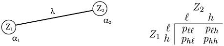
Figure 2. The n = 2 case with variables Z₁ and Z₂. (Left) The graph, showing the model parameters. (Right) The joint PMF.

THEOREM 3 (limiting probabilities, two-variable case). Let Z₁ and Z₂ be jointly distributed according to autologistic model f_Z, with graph and probability table as shown in Figure 2. Let $p_{\ell \ell }^{*}$, $p_{\ell h}^{*}$, $p_{h\ell }^{*}$, and $p_{hh}^{*}$ be the limiting probabilities in the table as λ → ∞.

a)  If f_Z is a standard model and α₁, α₂ take any fixed values, then:

        if ℓ + h > 0, $p_{hh}^{*}=1$

        if ℓ + h < 0, $p_{\ell \ell }^{*}=1$

        if ℓ + h = 0, $p_{hh}^{*}=\frac{e^{h({\alpha }_1+{\alpha }_2)}}{e^{\ell ({\alpha }_1+{\alpha }_2)}+e^{h({\alpha }_1+{\alpha }_2)}}$ and $p_{\ell \ell }^{*}=1-p_{hh}^{*}$

b)  If f_Z is a centered model and ℓ, h take any fixed values, then:

        if α₁ + α₂ > 0, $p_{\ell \ell }^{*}=1$

        if α₁ + α₂ < 0, $p_{hh}^{*}=1$

        if α₁ + α₂ = 0, $p_{hh}^{*}=p_{\ell \ell }^{*}=\frac{1}{2}$

PROOF: Considering Equation (11) with n = 2, we can define the un-normalized PMF as

$\begin{array}{l}g(z_1,z_2)=e^{{\alpha }_1{z}_1}{e}^{{\alpha }_2{z}_2}{e}^{(z_1{z}_2-{\mu }_2{z}_1-{\mu }_1{z}_2)\lambda },\end{array}$

where μ₁ and μ₂ are the centering adjustments of Z₁ and Z₂ according to Equation (12). Then the probability of a particular configuration (z₁,z₂) is

$\begin{array}{l}Pr(Z_1=z_1,Z_2=z_2)\\ =\frac{g(z_1,z_2)}{g(\ell ,\ell )+g(\ell ,h)+g(h,\ell )+g(h,h)}\\ =e^{{\alpha }_1{z}_1}{e}^{{\alpha }_2{z}_2}{\left[\frac{g(\ell ,\ell )+g(\ell ,h)+g(h,\ell )+g(h,h)}{e^{(z_1{z}_2-{\mu }_2{z}_1-{\mu }_1{z}_2)\lambda }}\right]}^{-1}.\end{array}$

We are interested in the limiting value of this probability in eight cases: four configurations of (z₁,z₂), for each of the two model types. Clearly, any of these probabilities will be nonzero only if the ratio in the square brackets above (call it R) remains finite as λ → ∞. All of the results of the theorem are found by considering how this ratio behaves (as a function of α₁, α₂, ℓ, and h) over the eight cases.

Consider for example the case of the (h,h) configuration under the centered model. For this case, after some algebraic manipulations, we have

$\begin{array}{l}R=e^{\ell ({\alpha }_1+{\alpha }_2)}{e}^{(\ell -h)(h+\ell -{\mu }_1-{\mu }_2)\lambda }\\ +e^{(\ell {\alpha }_1+h{\alpha }_2)}{e}^{(\ell -h)(h-{\mu }_2)\lambda }\\ +e^{(h{\alpha }_1+\ell {\alpha }_2)}{e}^{(\ell -h)(h-{\mu }_1)\lambda }+e^{h({\alpha }_1+{\alpha }_2)}.\end{array}$

The right hand side is a sum of four terms. The last term is finite and not a function of λ. The second and third terms approach zero as λ → ∞, since ℓ < h and h is greater than both μ₁ and μ₂. So the value of $p_{hh}^{*}$ depends on the sign of h + ℓ − μ₁ − μ₂. Using Equation (12) to write μ₁, μ₂ in terms of h, ℓ, α₁, and α₂, it can be shown that

$\begin{array}{l}sgn(h+\ell -{\mu }_1-{\mu }_2)=\text{ sgn}\left(e^{\ell ({\alpha }_1+{\alpha }_2)}-e^{h({\alpha }_1+{\alpha }_2)}\right),\end{array}$

which equals (1,−1,0) when α₁ + α₂ is (less than, greater than, equal to) zero. From this we conclude the results about $p_{hh}^{*}$ in part b) of the theorem. The remaining results are obtained similarly by working out R for the other cases and considering its limiting behavior. □

The theorem shows that for the standard model, the limiting probabilities are only reasonable when the coding is symmetric around zero. If the sum of the coding values is nonzero, either $p_{\ell \ell }^{*}$ or $p_{hh}^{*}$ gets all of the probability mass, and which configuration gets the mass depends only on the coding, not on the unary parameters. When ℓ + h = 0, the limiting probabilities make sense: either configuration can occur, with weight that depends on α₁ + α₂.

For the centered model, the limiting behavior does depend on α₁ + α₂, but it does so in a counterintuitive way. For α₁ + α₂ ≠ 0, the configuration that is opposite of the unary parameters' endogenous tendency receives all of the probability mass. Large positive values of the unary parameters (which should promote the occurrence of h states) lead to $p_{\ell \ell }^{*}$ in the limit. Large negative values lead to $p_{hh}^{*}$. Only at the midpoint between these scenarios, α₁ + α₂ = 0, does the limiting PMF take a reasonable form.

3.3.2. The General Case

In the general-n case it relatively straightforward to determine the limiting probabilities for the symmetric model. Combined with the n = 2 results it is possible to make the following statement.

THEOREM 4 (limiting probabilities, general case). Let n-vector Z be distributed according to standard autologistic model S_ℓ,h(α, λA) with ℓ + h = 0 and with a connected graph. Define ℓ = ℓ1 and h = h1. Then the two configurations z = ℓ and z = h are the only ones with nonzero probability as λ → ∞, and this holds regardless of the parameter values or the particulars of the graph. The limiting probabilities are

$\begin{array}{l}{p}_{\text{h}}^{*}=\frac{\text{exp}\left(h{\displaystyle \sum _{i=1}^n}{\alpha }_i\right)}{\text{exp}\left(h{\displaystyle \sum _{i=1}^n}{\alpha }_i\right)+\text{exp}\left(\ell {\displaystyle \sum _{i=1}^n}{\alpha }_i\right)}\text{ and }{p}_{\ell }^{*}=1-p_{\text{h}}^{*}.\end{array}$

Furthermore, the standard model with ℓ + h = 0 is the only autologistic model variant for which more than one configuration has positive limiting probability regardless of n, the graph structure, or the parameter values.

PROOF: The standard model has PMF

$\begin{array}{l}f\left(\text{z}\right)=\frac{\text{exp}\left({\text{z}}^T\alpha +\frac{\lambda }{2}{\text{z}}^T\text{A}\text{z}\right)}{{\displaystyle {\sum }_{\text{x}\in {C}}}\text{exp}\left({\text{x}}^T\alpha +\frac{\lambda }{2}{\text{x}}^T\text{A}\text{x}\right)}\\ =\frac{\text{exp}\left({\text{z}}^T\alpha \right)}{{\displaystyle {\sum }_{\text{x}\in {C}}}\text{exp}\left({\text{x}}^T\alpha \right)\text{exp}\left(\frac{\lambda }{2}{\text{x}}^T\text{A}\text{x}\right)\text{exp}\left(-\frac{\lambda }{2}{\text{z}}^T\text{A}\text{z}\right)}\\ =\frac{\text{exp}\left({\text{z}}^T\alpha \right)}{{\displaystyle {\sum }_{\text{x}\in {C}}}\text{exp}\left({\text{x}}^T\alpha \right)\text{exp}\left(\lambda {\displaystyle {\sum }_{{E}}}\left(x_i{x}_j-z_i{z}_j\right)\right)},\end{array}$

where ${C}$ is the set of 2ⁿ possible configurations. Letting d_ij = x_ix_j − z_iz_j, it is clear from the last line that for any chosen z, $\underset{\lambda \to \infty }{lim}f(\text{z})$ depends on the values of

$\begin{array}{l}{L}_{\text{x}}\equiv {\displaystyle \underset{\lambda \to \infty }{lim}}\text{exp}\left(\lambda {\displaystyle \sum _{{E}}}{d}_{ij}\right)\end{array}$

for all configurations $\text{x}\in {C}$. Considering all possible arrangements of (x_i,x_j) and (z_i,z_j) and remembering that we have set ℓ = −h, we find that

$\begin{array}{l}{d}_{ij}=\{\begin{array}{cc}0& \text{if}(x_i,x_j)=(z_i,z_j)\text{ or }(x_i,x_j)=-(z_i,z_j)\hfill \\ 2h^2& \text{if }{x}_i=x_j\text{but }{z}_i\ne z_j\hfill \\ -2h^2& \text{if }{x}_i\ne x_j\text{but }{z}_i=z_j.\hfill \end{array}\end{array}$

Now choose z = ℓ or z = h. These are the only two choices for which z_i = z_j for all edges (because the graph is connected). Then $\sum _{{E}}{d}_{ij}\le 0$ for every x, with equality only when x = ±z. Consequently L_x = 1 for x = ±z and L_x = 0 for all other x. From this we conclude that $p_{\text{h}}^{*}$ and $p_{\ell }^{*}$ are as given in the theorem, and therefore all other limiting probabilities must be zero.

The conclusion that the S_−h,h(α, Λ) model is the only variant with more than one positive limiting probability in general may be justified by counterexample. The n = 2 case (Theorem 3) provides counterexamples for all of the other AL model variants. □

Theorem 4 shows that the symmetric models, S_{−h, h}, are the only AL/ALR variants that always have reasonable and intuitive large-λ behavior.

3.4. Pseudolikelihood

Let z¹, …, z^m be a random sample drawn from an autologistic model with n vertices. The pseudolikelihood function is the product of the conditional probabilities,

$\begin{array}{ll}PL(\theta )={\displaystyle \prod _{j=1}^m}{\displaystyle \prod _{i=1}^n}Pr(Z_{ji}=z_{ji}|{{\text{z}}_{-i}}^j),& (21)\end{array}$

where θ = (α, λ) is the parameter vector and z_ji is the value of the ith variable in the jth observation. Equation (9) is used to compute the conditional probabilities.

Pseudolikelihood is an approximation to the true likelihood [32], and maximum pseudolikelihood (MPL) is widely used as a practical estimation method given the intractability of the partition function for large n.

Detailed consideration of the optimization of Equation (21) for all AL and ALR variants is beyond the scope of the present work, but the theorem below and the comments that follow are relevant to comparison of the centered and standard model types.

THEOREM 5 (pseudolikelihood for standard models). For the standard AL or ALR model with any coding and the simple smoothing assumption, the negative log pseudolikelihood is a convex function of its parameters.

PROOF: The proof is straightforward so most of the details are omitted. Consider the AL model. Note from Equations (8) and (9) that conditional probability for variable i is a function only of parameters α_i and λ. Therefore we can define $q_{ji}({\alpha }_i,\lambda )\equiv -log(Pr(Z_{ji}=z_{ji}|{{\text{Z}}_{-i}}^j))$ and write the negative log pseudolikelihood function as

$\begin{array}{l}-logPL(\theta )={\displaystyle \sum _{j=1}^m}{\displaystyle \sum _{i=1}^n}{q}_{ji}({\alpha }_i,\lambda ).\end{array}$

The function is convex if every q_ji(·) is a convex function of its parameters. A function of r parameters is convex if it is convex along every line in the parameter space [33], so define u_ji(t) = q_ji(_αi1 + t_αi2, λ₁ + tλ₂). Convexity is proven by finding the second derivative of u_ji(t) with respect to t and observing that it is positive for any choice of _αi1, _αi2, λ₁, λ₂, for any coding and for all i, j. Convexity for the ALR case follows because the composition of a convex function with a linear one (here, ${\alpha }_i={\text{x}}_i^T\beta$) is convex. □

This convexity result indicates that obtaining parameter estimates by MPL should be straightforward for any standard variant (including both the traditional zero/one model and the symmetric model). Unfortunately the same can not be said for centered models. The centering term μ_j is a non-convex function of α_j. Additionally, in the centered model the ith conditional probability is a function of not only α_i and λ, but also of parameters α_j, j ~ i. Thus we expect more complications with obtaining good parameter estimates even using the simple MPL framework. Indeed, multiple local optima have been observed in the MPL function even for n = 2 examples, and for larger problems, numerical optimizers may return different MPL parameter estimates depending on the starting point of the search.

4. Numerical Results

This section provides numerical examples to complement the theoretical results and shed more light on the differences among the autologistic variants. The first example focuses on better understanding of parameter interpretation in AL models for the n = 2 case. The second explores the qualitative differences among the variants in a spatial-data regression setting at larger scale (n = 900). The third quantifies the distance between the most important ALR variants in a network-structured regression scenario with n = 16. After these constructed examples, an analysis of the H. vulgaris data set is presented.

4.1. Parameter Interpretation in the Two-Variable Case

In section 2.5 it was argued that the autologistic model invites a natural interpretation of its parameters as defining a balance between the unary or endogenous part, and the neighborhood effects. To examine whether this interpretation holds for different AL variants, we first restrict our attention to the effects that two variables have on each other.

4.1.1. Expected Neighbor Effect

Consider two variables Z_i and Z_j that may be part of a larger graph. The log odds expression (10) for Z_i, conditional on its neighbors, involves the neighbor sum s_i. The contribution of Z_j to this sum is S_i = λ_ij(Z_j − μ_j). Its expectation is

$\begin{array}{ll}E[S_i]=\{\begin{array}{cc}{\lambda }_{ij}{M}_j& \text{for the }{S}_{0,1}\text{ model}\\ {\lambda }_{ij}(M_j-{\mu }_j)& \text{for the }{C}_{0,1}\text{ model}\\ {\lambda }_{ij}(2M_j-1)& \text{for the }{S}_{-1,1}\text{ model}\end{array},& (22)\end{array}$

where M_j is the marginal probability Pr(Z_j = h). It depends on unary parameter α_j as well as on Z_j's neighbors and the strength of their association with Z_j.

The relationships in Equation (22) are shown graphically in Figure 3. For the S_0,1 model, the expected neighbor effect is always positive—increasing the log odds that Z_i takes the high level—regardless of M_j. This is another way of expressing the asymmetry inherent in the standard zero/one model. The centered model corrects this problem, in that E[S_i] can take negative values, but the range of possible neighbor effects is now coupled to α_j, through μ_j. This introduces a type of antisymmetry, where larger μ_j values shift the range of possible neighbor effects downward and smaller μ_j values shift it upward. This antisymmetry is the source of the counterintuitive large-λ behavior described in Theorem 3.

FIGURE 3

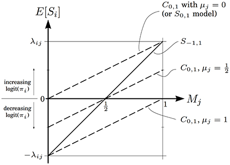
Figure 3. Expected value of the neighbor effect of variable j on variable i, as a function of M_j, the marginal probability that Z_j takes the high level. The solid line is for the symmetric model, and dashed lines are for the centered model with different μ_j values. The line for the standard zero/one model coincides with the uppermost dashed line.

The symmetric S_{−1, 1} model, by contrast, resolves the asymmetry problem of the zero/one model without introducing extra complexities. The expected neighbor effect varies linearly from −λ_ij to λ_ij, crossing through zero when M_j = 0.5. This is a natural crossing point: when Z_j is equally likely to take either state, its average effect on Z_i is zero. The centered model only exhibits similar behavior when μ_j = 0.5.

4.1.2. Marginal Probability

Next, consider the n = 2 case previously encountered in Figure 2. There are two random variables Z₁ and Z₂, and three parameters α₁, α₂, and λ. One way to better understand the parameters' roles is to study how they influence the probability of the event {Z₁ = h}.

It is helpful to consider the effects of the unary parameters not through α₁ and α₂ directly, but rather through the endogenous probabilities p₁ and p₂, which are monotone functions of them:

$\begin{array}{l}{p}_i=\frac{e^{h{\alpha }_i}}{e^{\ell {\alpha }_i}+e^{h{\alpha }_i}},i=1,2.\end{array}$

This eliminates a scaling difference that would otherwise confuse the comparison of models with different coding. Note that p_i = 0.5 corresponds to α_i = 0.

Figure 4 shows contour plots of Pr(Z₁ = h) as a function of p₁ and p₂, for the S_0,1, C_0,1, and S_{−1, 1} models. Each row of contour plots in the figure is for a single model variant. The λ values for each variant are evenly spaced between 0 and some maximum value. The maximum values were chosen such that |Pr(Z₁ = h) − 0.5| = 0.4 when p₁ = 0.5 and p₂ = 0.95 (this is a point at which the neighbor effect of Z₂ on Z₁ is large). The C_{−1, 1} model was also plotted but is not shown. Although its maximum λ value is different, its contours are identical to those of the C_0,1 model.

FIGURE 4

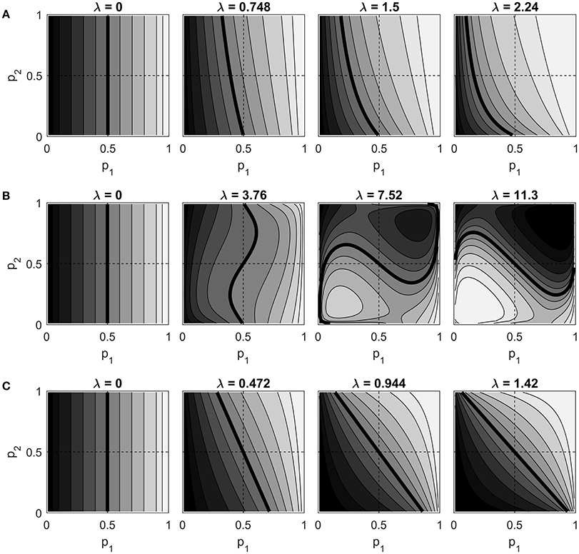
Figure 4. Contour plots of Pr(Z₁ = h) vs. p₁ and p₂ for different λ values, for (A) the S_0,1 model, (B) the C_0,1 model, and (C) the S_{−1, 1} model. Contour lines are drawn at probabilities 0.05, 0.1, 0.2, …, 0.9, 0.95, with lighter shades of gray representing higher probabilities. The probability 0.5 contour is thicker than the rest. Dashed lines are drawn horizontally and vertically through the point (0.5, 0.5), which corresponds to α₁ = α₂ = 0.

At λ = 0, the variables are independent and all three variants exhibit the same behavior: Pr(Z₁ = h) increases monotonically with p₁, unaffected by p₂. As λ increases, we might expect (under the natural interpretation) that this probability should remain an increasing function of p₁, but also become an increasing function of p₂ as well, due to the neighbor effect. The figure shows that both of the standard models do in fact demonstrate this expected behavior. The S_0,1 model does so while exhibiting its asymmetry: as λ increases, the marginal probability increases throughout the plane, even in areas where both p₁ and p₂ are less than one half. The S_{−1, 1} model, on the other hand, gives the expected behavior while maintaining a marginal probability of 0.5 at p₁ = p₂ = 0.5 at every choice of λ.

Turning to the centered model (row B in the figure), it is clear that this model does not show the expected behavior. In this model, increasing p₂ may either increase or decrease the marginal probability, depending on where one is in the (p₁, p₂) plane. While the centered model does maintain Pr(Z₁ = h) = 0.5 for all λ when p₁ = p₂ = 0.5, we again see counterintuitive behavior when λ becomes large. The marginal probability that Z₁ = h is nearly zero in the first quadrant, precisely where both endogenous probabilities are large. Also note that a much larger λ value is required to get a strong neighbor effect. This is a direct consequence of the centering adjustment, which subtracts the independence expectation from each Z_j in the neighborhood sum.

4.1.3. Concordance Probability

Continuing with the same example, we can also consider the probability that Z₁ and Z₂ are concordant, that is, Pr(Z₁ = Z₂). The log odds of this probability are given in Figure 5, as a function of λ, for the same three variants at different (p₁, p₂) combinations. The log odds has been chosen to highlight an interesting difference between the symmetric model and the other variants. For a symmetric model, the odds of event {Z₁ = Z₂} are

$\begin{array}{l}\frac{Pr(Z_1=Z_2)}{Pr(Z_1\ne Z_2)}=e^{2\lambda h^2}\frac{e^{2h({\alpha }_1+{\alpha }_2)}+1}{e^{2h{\alpha }_1}+e^{2h{\alpha }_2}},\end{array}$

which factorizes into a part depending on λ alone and another depending on α alone. As a result the log odds of the event, for any fixed (p₁, p₂), is a linear function of λ with slope 2h². This invites a simple interpretation of λ as an association parameter: a unit change of λ will increase the log odds of the two variables taking the same state by 2h², regardless of the values of the unary parameters. This is visible in row (C) of the figure.

FIGURE 5

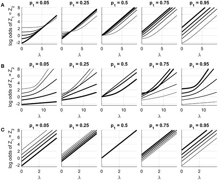
Figure 5. Log odds of event {Z₁ = Z₂} when n = 2, as a function of λ at different (p₁, p₂) combinations for (A) the S_0,1 model, (B) the C_0,1 model, and (C) the S_{−1, 1} model. Each subplot uses a fixed value of p₁ as shown. Line thickness corresponds to the value of p₂: from thinnest to thickest, p₂ = 0.05, 0.25, 0.5, 0.75, 0.95. The horizontal plot range was chosen so that the log odds at p₁ = p₂ = 0.5 varied from 0 to 8 for each model.

The S_0,1 model and the centered variants (rows A and B) do not admit such an interpretation. For these two models the log odds curves show nonlinearities that change depending on the values of p₁ and p₂. In both cases the curves are difficult to explain intuitively. In row (A), we see that the curves for (p₁ = 0.05, p₂ = 0.05) are not the same as the curves for (p₁ = 0.95, p₂ = 0.95). This is hard to justify given that the two cases differ only by the labeling of the high and low states. In row (B) we see that the shapes of the curves depend in a complex way on p₁ and p₂. For example, the initial slope of the curve is greatest at (p₁ = 0.5, p₂ = 0.5), and much smaller when (p₁ = 0.95, p₂ = 0.95). This implies that increasing λ from zero will more strongly influence variables that are both indifferent about their state than it will variables that are both strongly biased to the same state.

4.2. A Spatial Regression Example

Now consider a larger example with a regression component. Let Z be a vector of n = 900 binary variables, jointly distributed according to an ALR model. The graph structure for the model is a regular 30 × 30 lattice; each interior node has four neighbors.

The graph is positioned in space such that it covers the unit square, with the lower left vertex at (0, 0) and the upper right one at (1, 1). Let the spatial coordinates of variable i be (x_i1, x_i2). For simplicity, let these spatial coordinates (plus an intercept term) be the predictor variables for regression. Defining X to be a 900 × 3 matrix of covariates, with ith row ${\text{x}}_i^T=(1,x_{i1},x_{i2})$, the ith variable's unary term becomes

$\begin{array}{l}{\alpha }_i\equiv {\text{x}}_i^T\beta ={\beta }_0+{\beta }_1{x}_{i1}+{\beta }_2{x}_{i2}.\end{array}$

For this example, we fix β = (−2, 2, 2)^T throughout and explore the effect of λ on three variants: S_0,1(Xβ, λA), C_0,1(Xβ, λA), and S_{−1/2, 1/2}(Xβ, λA). The symmetric model uses {−1/2, 1/2} coding to ensure that when λ = 0, it is equivalent to variants coded {0, 1}.

The present example is very similar to the simulation setting used by both Caragea and Kaiser [24] and Hughes et al. [25]. When λ = 0, every variant gives the same logistic regression model with endogenous probabilities varying smoothly over the unit square, from approximately 0.12 in the lower left corner to about 0.88 in the upper right. The diagonal separating these two corners has endogenous probability 0.5. Figure 6 shows these probabilities as a grayscale image. Such displays are referred to as marginal probability maps; by convention they will plot Pr(Z_i = h) and use lighter shades of gray to represent higher probability. The graph corresponding to Z is also shown on the figure.

FIGURE 6

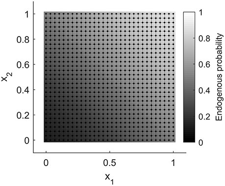
Figure 6. The graph for the ALR example, with Pr(Z_i = h|λ = 0) displayed as an image beneath the vertices.

For each model, 500 random samples were drawn at each of ten λ values equally spaced from 0 to 2.5. Estimates of the marginal probabilities were obtained from the samples by counting the proportion of draws for which each variable took its high level. Random draws were obtained by perfect sampling, which is relatively straightforward to implement for AL/ALR models (see [25], and references therein; also [34]).

Figure 7 shows the configurations of two random samples, as well as the estimated marginal probability maps, for each model at each λ. The differences among the models are clear, and agree with the observations in the n = 2 case. In the standard {0,1} model, increasing λ increases the chance of observing the high state, at every vertex, regardless of covariate values. In the centered model, smaller λ values (up to about 0.75) have only a minor effect on the probability map. At larger λ values more clustering of the high and low states is visible, but the low states occur at vertices where the endogenous probability is high (and vice versa). For the symmetric model, increasing λ causes the probability map to gradually separate around the diagonal, with (low, high) states occurring where the endogenous probability is (low, high).

FIGURE 7

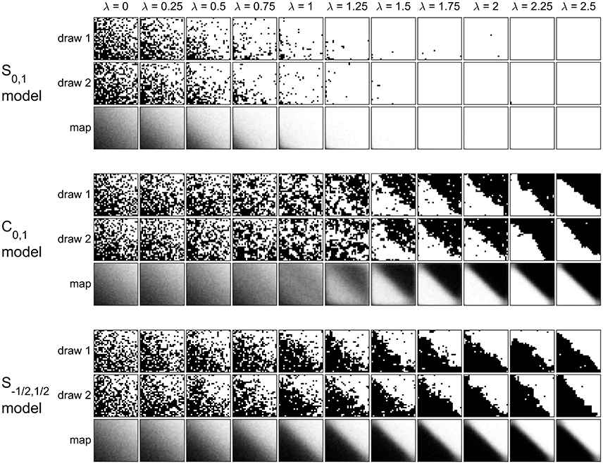
Figure 7. Effect of λ on three model variants when β = (−2, 2, 2)^T. Two randomly-drawn configurations are shown for each model at each λ value, along with the estimated marginal probability map. The realizations are displayed as images with black and white pixels representing the low and high states, respectively.

To more directly assess the effect of λ on neighbor interactions, we can consider not just the vertices of the graph but the edges. For any group of edges, the probability of edge concordance can be estimated by the proportion of times those edges were concordant over the 500 random samples. To see how the endogenous probabilities modulate the effect of λ on concordance, partition the graph into two subgraphs: ${{G}}_1=\{Z_i:p_i\le \frac{1}{3}\mathrm{\text{or}}{p}_i\ge \frac{2}{3}\}$ and ${{G}}_2=\{Z_i:\frac{1}{3}<p_i<\frac{2}{3}\}$. Subgraph ${{G}}_1$ includes edges in the lower left and upper right of the unit square, where both endogenous probabilities are strongly biased toward one state or the other. Subgraph ${{G}}_2$ includes edges near the diagonal, where the average endogenous probability of the edge is not far from one half.

Figure 8 shows the estimated concordance probability of edges in ${{G}}_1$ and ${{G}}_2$, for the C_0,1 and S−1/2, 1/2 models. In the symmetric model, the effect of λ is roughly the same for edges in either group. For the centered model, increasing the association parameter has a fairly strong effect on ${{G}}_2$ but a very small effect on ${{G}}_1$. This effect can also be observed by careful inspection of Figure 7 for λ ≤ 1. For the centered model, the smoothing effect of λ is focused on the parts of the graph where p_i + p_j is close to one. This is consistent with the results previously seen in Figure 5.

FIGURE 8

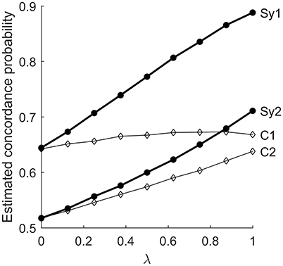
Figure 8. Estimated concordance probability of edges in subgraphs ${{G}}_1$ and ${{G}}_2$, vs. λ. C1 and C2 are the results for subgraphs 1 and 2, respectively, using the centered zero/one model. Sy1 and Sy2 are the corresponding curves for the symmetric model.

4.3. A Network Regression Example

The preceding two examples have focused on parameter interpretation, but it is not always essential to have a readily interpretable model. In statistical learning applications, for example, out-of-sample predictive accuracy may be the dominant objective. In such a case, there is little reason to be concerned about which variant is used, as long each variant's parameters can be changed to produce nearly equivalent predictive models. To see whether any concern is justified, we must address the question of how far apart two distribution families defined by ALR models can be.

The approach taken here is to let the symmetric model be the reference distribution family. Instances of this model were generated with random graphs, random covariates, and fixed parameters. Each such instance formed the baseline or target model for a single experimental run. Numerical optimization was then used to find the parameter settings of the S_0,1 and C_0,1 models that minimize a measure of statistical distance between them and the target model.

Take the Hellinger distance as our distance measure. If M₁ and M₂ are two ALR models with n vertices, which respectively assign probabilities $\text{w}={(w_1,w_2,\dots w_{2^n})}^T$ and $\text{v}={(v_1,v_2,\dots v_{2^n})}^T$ to the 2ⁿ possible configurations, the Hellinger distance between the models is $\frac{1}{\sqrt{2}}{\Vert \sqrt{w}-\sqrt{v}\Vert }_2$, where the square roots inside the norm are taken componentwise. It varies between zero (when the models are equivalent) and one (when the sets of configurations given positive probability by the models are disjoint). Models that have Hellinger distance not close to zero can not be considered reasonable approximations of one another as predictive models.

For this example we consider graphs and covariates that have a network structure, rather than a spatially-referenced one. Graphs were generated according to a preferential attachment scheme [35, 36]. For each graph, an initial set of m₀ fully connected vertices is first created, and additional vertices are added sequentially until there are n nodes in total. Each new node is connected by edges to m existing nodes, selected randomly with weights that are proportional to their degree. In this experiment we consider two cases. Case 1 has m₀ = 4 and m = 1. In this case the graph is structured as tree branches connected to the initial fully-connected four nodes. Case 2 has m₀ = m = 2. This case has more connectivity throughout the graph.

The baseline models were generated as follows. Fix n = 16, which is sufficiently small to allow direct calculation of the Hellinger distance. Set λ = 0.25, and generate 200 graphs for each of Case 1 and Case 2. For each graph, assign to each vertex a linear predictor α_i = β₀ + β₁x_i, where x_i, i = 1…16 are drawn independently from a standard normal distribution. Each graph then has its own adjacency matrix A and covariate matrix X; take the S_−1,1(Xβ, λA) model with β₀ = 0 and β₁ = 1 as the target model corresponding to that graph. Repeat this process for λ = 0.5, 0.75, 1.0, 1.25, and 1.5.

Figure 9 gives examples of graphs generated from the two cases. The baseline models correspond to a situation where the endogenous probabilities of neighbor variables are noisy and uncorrelated. Models with larger λ values will put higher probability on configurations that have clusters of high or low values, with cluster size and location modulated by the endogenous probabilities. In the limit as λ → ∞, the two saturated states Z = −1 and Z = 1 will get all of the probability mass, according to Equation (20).

FIGURE 9

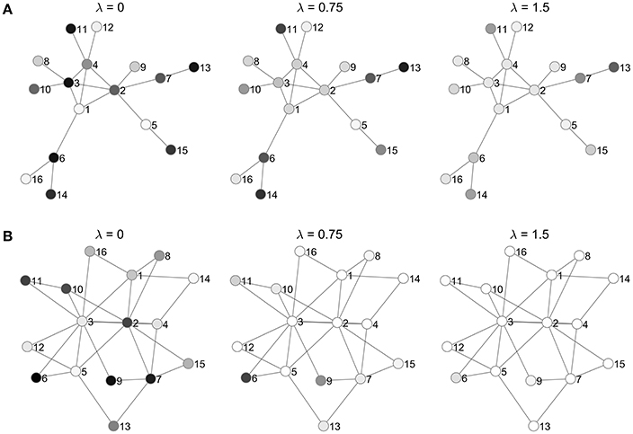
Figure 9. Examples of symmetric ALR models obtained by randomly generating a graph and covariates according to (A) Case 1 and (B) Case 2 as described in the text. Each model is shown for three λ values, to illustrate the neighborhood effect. Nodes are shaded to indicate their marginal probability of taking the high level (lighter shades indicate higher probability).

Numerical optimization was performed to find models ${\text{S}}_{0,1}(\text{X}\widehat{\beta },\widehat{\lambda }\text{A})$ and ${\text{C}}_{0,1}(\text{X}\tilde{\beta },\tilde{\lambda }\text{A})$ that minimize the Hellinger distance to each target. Figure 10A gives violin plots [37] of the distances. Each “violin” in the plot is based on an unequally-spaced histogram with bin edges at the sample quintiles. The median value is indicated by a dot.

FIGURE 10

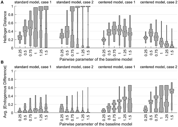
Figure 10. The distribution of (A) Hellinger distance to the baseline model and (B) average absolute difference in endogenous probability vs. the baseline model, for the minimum-distance models in the network example.

The figure reveals striking differences between the nearest models. All but three of the experimental settings produce median distances greater than 0.2, and many are greater than 0.4. This means that the S_0,1 and C_0,1 models cannot apportion probability mass to configurations in a manner very similar to the symmetric model. The distances also have high variability. This indicates that the ability of the standard and centered variants to approximate the symmetric model is strongly influenced by the random aspects of the target model: the graph structure and the covariate values.

The distribution of distances for the standard zero/one model becomes bimodal as λ gets large. Inspection of the data showed a strong relationship between the sum of the covariates and the Hellinger distance. Larger negative values of ∑x_i corresponded to larger distances. In this situation, the target model puts more weight on configurations with many low states, but the S_0,1 model can not easily do the same, because increasing λ always promotes the high state.

The distributions of the centered models' distances are not bimodal, but they also exhibit considerable variation. For Case 2 target models, the median Hellinger distance of the C_0,1 model begins to decrease sharply when the target model's association parameter is greater than one half. One reason for this is that the probability mass of the target distribution begins to concentrate around a small number of configurations near the saturated ℓ and h states, essentially making it easier to approximate the distribution. This effect is stronger in Case 2 than in Case 1, because the higher connectivity of the graph in Case 2 strengthens the neighborhood effect at a given λ level.

This example demonstrates that we can not treat the different ALR variants as interchangeable, even approximately, and even if we are only concerned with predictive modeling. If we are also interested in parameter interpretation, then the regression parameter estimates are of particular interest, since they always define the endogenous probabilities. To compare the linear predictors of the models, we can calculate the average absolute difference of the 16 endogenous probabilities, relative to the target model. Figure 10B shows the distribution of these averages for the experimental runs. For the centered model, we see that when the Hellinger distances are small, the endogenous differences are large. This shows that when λ > 0, we can not find a situation where the centered and symmetric models provide similar probability distributions and similar interpretations at the same time.

4.4. Analysis of the Hydrocotyle Vulgaris Data

We now return to the H. vulgaris data to see how the differences among the ALR variants can manifest themselves in a real application. The S_0,1, C_0,1, and S_{−1/2, 1/2} models were all fit to the data using a four-nearest-neighbor graph and the MPL method. Optimization of the pseudolikelihood was attempted from multiple random starting points. For the two standard models, the same solution was found each time (unsurprisingly, given Theorem 5). For the centered variant, three locally-optimal solutions were found; the one with greatest log pseudolikelihood was assumed to be the global optimum. Let β₀, β₁, and λ be the intercept, the coefficient of altitude, and the association parameter, respectively.

Results of the analysis are shown in Figure 11, which shows the estimated marginal probability maps, and Table 1, which gives the coefficient estimates. The table includes standard errors obtained by the parallel parametric bootstrap as in Hughes et al. [25]. A column labeled “impact” is also given for each parameter. This column holds the covariate impact, as defined in Bardos et al. [23]. In that work, the authors observed a covariate amplification/parameter attenuation effect in auto-models, where (relative to logistic regression) smaller coefficient magnitudes were required to obtain similar observed effects on the fitted values. The impact is an alternative measure of a covariate's influence on the response, intended to be informative despite structural differences across models. The impact is obtained by setting the coefficient in question to zero and re-evaluating the marginal probabilities of the model. The average (across vertices in the graph) of the absolute change in marginal probability is the impact.

TABLE 1

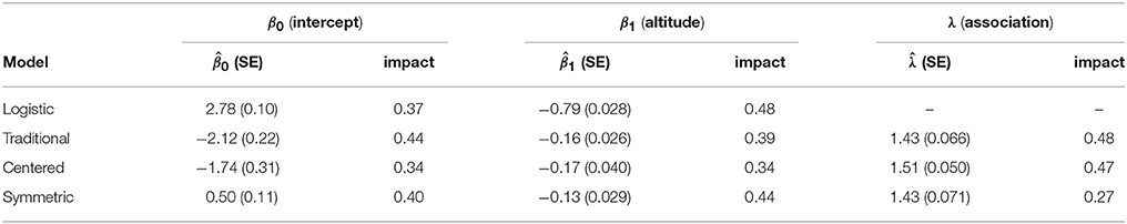
Table 1. Parameter estimation results for the H. vulgaris data.

FIGURE 11

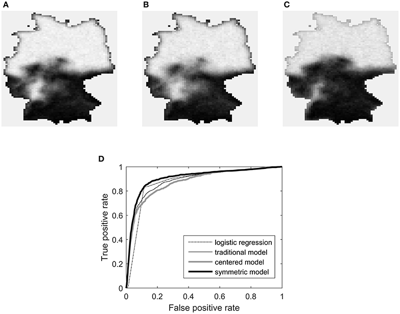
Figure 11. Results of ALR analysis of the H. vulgaris data. The top row shows marginal probability maps for (A) the traditional S_0,1 model, (B) the centered model, and (C) the symmetric model. Plot (D) gives the receiver operating characteristic curves for the three models as well as ordinary logistic regression.

If we look only at the magnitudes of $\widehat{\lambda }$ and ${\widehat{\beta }}_1$, the three ALR models appear quite similar. All have $\widehat{\lambda }\approx 1.5$, indicating strong spatial association. All have ${\widehat{\beta }}_1\approx -0.15$, which is much smaller than the logistic regression value of −0.79 (evidence of the parameter attenuation phenomenon).

Interpretation difficulties begin to arise for the S_0,1 and C_0,1 models, however, when we consider ${\widehat{\beta }}_0$. Both models assign large negative values to the intercept, suggesting that when the altitude is zero everywhere, the species should be largely absent. This is contrary to the observed facts, where species presence has a clear association with low elevation. The coefficient of altitude (a positive quantity) is also negative in both models, leaving no obvious way for species presence to take a high probability. Indeed, the maximum endogenous probability over the entire map for either model is less than 0.2. How is it, then, that the fitted models assign high probability in the northern part of the map? It is only because λ is large enough to distort the meaning of the regression part of the model. This is reflected in the large value of impact for λ in these two models. Adding the neighbor effect to either model has a drastic effect on the fitted values everywhere in the map.

Contrast this with the interpretation of the symmetric model. Its coefficients have the same signs as, and magnitudes roughly proportional to, the logistic regression model. The median endogenous probability across the map is 0.49 for logistic regression and 0.51 for the symmetric model. The neighbor effect promotes the marginal probabilities to intensify (toward either zero or one) if local regions' endogenous tendencies agree. As a result the impact of λ is much lower than it is for the other ALR variants. Compared to the centered model, the regression parameters have much higher impact values and much more precise estimates.

The probability maps support the notion that the symmetric model is more appropriate for these data. Its marginal probabilities more closely match the altitude map and the obeserved pattern of species presence seen in Figure 1. There also appears to be an edge effect in the northern half of map for the traditional and centered models, which is not present in the symmetric case.

A more structured method of comparing goodness-of-fit and potential predictive power is to produce a receiver operating characteristic curve for each model. This was done for the same data by Bardos et al. [23], but only for logistic regression and the traditional S_0,1 model. In Figure 11D a similar plot is shown with the centered and symmetric models included. The symmetric model dominates the other three models.

5. Discussion

The preceding sections provided results about model equivalence and parameter interpretation for autologistic models. They have important implications for analysts considering using these models.

The main results about equivalence apply for models with nonzero association matrices and arbitrary full-rank covariate matrices. They are:

• Every AL model (centered or standard, any coding) is equivalent to any chosen standard AL model.

• Two standard ALR models are equivalent if their codings differ by a positive scaling factor (otherwise they are not).

• Any two centered ALR models with different codings are not equivalent.

• Any given standard ALR model is not equivalent to any given centered ALR model, even if their coding is the same.

It was shown by example that the statistical distance between non-equivalent models can be large, making model choice a matter of practical consequence. Given the known limitations of the S_0,1 model, the choice is mainly between the centered {0,1} and symmetric {−h, h} variants.

5.1. A Case for the Symmetric Model

The centered and symmetric models can be thought of as competing alternatives, each aiming to remedy the parameter interpretation problem of the traditional S_0,1 model.

The centered model modifies the algebraic form of the traditional model. It does so in a manner analogous to Gaussian models, with the goal of making the regression parameters directly control the marginal probabilities. This goal is not achievable for dichotomous variables, however, because the covariance of any two such variables is functionally related to their marginal probabilities. As a result, centering achieves its goal only approximately, and only over a restricted region of the parameter space.

In exchange for this modest benefit, the centered model introduces extra analytical and computational difficulties. One such difficulty is non-convexity of the pseudolikelihood. Another, more critical, one is the counterintuitive behavior of the model when association is strong. This undesirable side effect was not noted in the initial articles about the centered model—perhaps because only λ values in the range [0, 1] were considered—but it has been subsequently documented [38]. It is not easy to say in advance when it will become problematic for a specific data set and graph structure, but when it does, any interpretation benefit will surely be lost. Users of the centered model must be prepared to check carefully for the problem after parameter estimation.

The preceding sections have demonstrated that the problems with the traditional model are not due to its algebraic form or its lack of centering, but simply due to the asymmetry of the {0, 1} coding. The symmetric model only changes the coding, but this change is sufficient to allow a very natural interpretation of the parameters. The regression parameters determine the endogenous structure, and λ provides a balance between the endogenous structure and the neighbor effect. This favorable interpretation remains the same regardless of the strength of association (and, by Theorem 4, the symmetric variants are unique in this regard). The symmetric model resolves the problems with the traditional model in a simple way, without introducing extra difficulties. Indeed, one could argue that if the symmetric model had been proposed first, there would be little reason to consider the centered model.

The H. vulgaris example demonstrated both the deficiencies of the centered model and the advantages of the symmetric one. Using the centered model, the regression parameters lacked a reasonable interpretation, and this happened without other obvious signs of problems with the model (the estimate of λ was not unreasonably large, and there was not dramatic lack of fit). The symmetric model, on the other hand, provided a more natural parameter interpretation with a closer connection to logistic regression. At the same time it had better fit, larger covariate impact, and more precise regression parameter estimates.

The ultimate arbiters of model quality in practice are goodness-of-fit and suitability for modeling objectives. It is not possible to declare in advance that a single variant is preferable in all circumstances. Nevertheless, all of the results of the present work point to the symmetric model as the autologistic variant with the most desirable properties. Future researchers are strongly recommended to consider the symmetric model as the starting point for their AL/ALR analyses, unless the physical data-generating process has clear links to an alternative model.

5.2. The Symmetric Model with Bernoulli Responses

The symmetric S_−h,h model could be criticized for two minor drawbacks. First, the value of h is not specified. Second, since the coding is not {0, 1}, we can not say that E[Z_i] = Pr(Z_i = 1). The latter drawback denies us the convenience of directly using sample averages to approximate probabilities, as we can do with Bernoulli-distributed random variables.

Both of the drawbacks can be eliminated by performing a transformation to make the symmetric model use the more familiar zero/one binary variables. If random variables Z are distributed according to the recommended S_−h,h(Xβ, Λ) model, with h unspecified, transforming Z into Y according to

$\begin{array}{l}\text{Y}=\frac{1}{2h}\text{Z}+\frac{1}{2}\text{1}\end{array}$

will leave f_Y equivalent to f_Z, but with support {0, 1}ⁿ instead of {−h, h}ⁿ. Note that this is a proper transformation of variables, not a just a change of coding (see Appendix A). The model has not been fundamentally altered.

Table 2 shows the model formulae for Z and Y as just described. It may be taken as a summary of the recommended model, in two equivalent forms. The parameters in f_Y have been written as γ = 2hβ and Ω = 4h² Λ to suppress the dependence on h, but parameter interpretation is not affected. The f_Z form makes the roles of the parameters most clear, while the f_Y form does not depend on h and shows the model as a natural extension of logistic regression. Since the use of the model as a spatial extension of logistic regression is very common, we may anticipate that f_Y, with conditional logit

$\begin{array}{l}\mathrm{\text{logit}}({\pi }_i)={\text{x}}_i^T\gamma +{\displaystyle \sum _{j~i}}{\omega }_{ij}(y_j-\frac{1}{2})\end{array}$

and Y_i ∈ {0, 1}, will be the most user-friendly form. It is interesting (but perhaps not surprising, in light of Figure 3) to note that f_Y looks the same as the centered ALR model, but with the centering adjustment equal to $\frac{1}{2}\text{1}$ instead of μ_γ.

TABLE 2

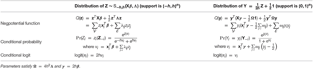
Table 2. Model formulae for the symmetric ALR model, in two forms.

5.3. Final Remarks

Having now chosen the symmetric model as a preferred variant, and realized that the ALR variants are not equivalent, it is suitable to begin considering questions of parameter estimation and model performance for the symmetric model, along the lines of Dormann [39] (which used the standard zero/one model) and Hughes et al. [25] (which used the centered zero/one model). Measures of goodness-of-fit should be a significant part of any such studies. Further investigation along this line is planned for the future.

While it is true that different ALR variants are non-nested models, the general form of section 2.3 does link the variants as part of a larger family. This suggests the idea of estimating the coding along with the other parameters. One could, for example, consider only the standard variants, let ℓ = −1 (for identifiability) and then estimate h from the data. This is somewhat of a technical curiosity, since it is hard to imagine what meaning one would assign to h; but it would make the model more flexible.

It would be of considerable practical interest to extend the ALR model beyond the simple smoothing assumption to an adaptive smoothing model, where the pairwise parameter is a function of the neighbor variables' states (and possibly covariates). This is also known as a metric MRF approach [30]. The standard model with plus/minus coding should again be best suited to this extension, which would greatly increase model flexibility. Initial exploration of this approach has shown promise.

The autologistic model is a pairwise MRF model; it is possible to construct MRFs for binary responses where cliques of more than two variables contribute to the negpotential function. In this more general case, the crucial aspect of model construction is to design the clique potential functions (ψ_m in Equation 2) in a way that reflects the model's intended purpose. Being aware of the potential impact of coding changes, it would be wise to construct the clique potentials in a way that is invariant to the coding. If this is not possible, the role of coding should be considered carefully to determine the best choice.

Another extension of the AL/ALR models is to the case of categorical responses with more than two levels. Again, the crucial task is the appropriate design of the clique potentials. When there are three or more levels, dependence on the coding is likely to increase in complexity. The multilevel logistic model [7, 21] is one extension of the AL model to handle more than two levels. It overcomes the coding problem by simply checking whether every variable in a clique takes the same value. If all of the values are equal, the clique potential is +1; otherwise, it is −1. The result is a negpotential function very similar to that of the symmetric AL model. Further development of models of this type, including a regression component and a clear connection to standard multinomial logistic (softmax) regression, is a potentially fruitful avenue for future work.

Finally, it is possible that the simple observation behind this work—that even a linear transformation of response coding may be a non-trivial operation—could have implications in other use cases as well. Probabilistic graphical models find application in a variety of pattern recognition and deep learning architectures, which are continually being extended in various directions. It is advisable to pay attention to variable coding, to determine if it can change the nature of the model, or be exploited to improve performance.

Author Contributions

The author confirms being the sole contributor of this work and approved it for publication.

Conflict of Interest Statement

The author declares that the research was conducted in the absence of any commercial or financial relationships that could be construed as a potential conflict of interest.

Acknowledgments

The author would like to thank Charmaine Dean for providing the application that led to the present work, and for helpful comments on a draft of this manuscript.

References

1. Besag JE. Nearest-neighbour systems and the auto-logistic model for binary data. J R Stat Soc Ser B (1972) 34:75–83.

Google Scholar

2. Besag J. Spatial interaction and the statistical analysis of lattice systems. J R Stat Soc Ser B (1974) 36:192–236.

Google Scholar

3. Kaiser MS, Cressie N. The construction of multivariate distributions from Markov random fields. J Multiv Anal. (2000) 73:199–220. doi: 10.1006/jmva.1999.1878

CrossRef Full Text | Google Scholar

4. Baxter RJ. Exactly Solved Models in Statistical Mechanics. London, UK: Academic Press Limited (1982).

Google Scholar

5. Cipra BA. An introduction to the ising model. Am Math Monthly (1987) 94:937–59. doi: 10.2307/2322600

CrossRef Full Text | Google Scholar

6. Geman S, Graffigne C. Markov random field image models their applications to computer vision. In: Proceedings of the International Congress of Mathematicians. Vol. 1. Berkeley, CA (1986). p. 2.

Google Scholar

7. Li SZ. Markov Random Field Modeling in Image Analysis. London, UK: Springer (2009).

Google Scholar

8. Blake A, Kohli P, Rother C, editors. Markov Random Fields for Vision Image Processing. Cambridge, MA: MIT Press (2011).

Google Scholar

9. Hinton GE. Boltzmann machine. Scholarpedia (2007) 2:8. doi: 10.4249/scholarpedia.1668

CrossRef Full Text | Google Scholar

10. Cox DR. The analysis of multivariate binary data. J R Stat Soc Ser C (1972) 21:113–20. doi: 10.2307/2346482

CrossRef Full Text | Google Scholar

11. Zhao LP, Prentice RL. Correlated binary regression using a quadratic exponential model. Biometrika (1990) 77:642–8. doi: 10.1093/biomet/77.3.642

CrossRef Full Text | Google Scholar

12. Cox DR, Wermuth N. A note on the quadratic exponential binary distribution. Biometrika (1994) 81:403–8. doi: 10.1093/biomet/81.2.403

CrossRef Full Text | Google Scholar

13. Dai B, Ding S, Wahba G. Multivariate bernoulli distribution. Bernoulli (2013) 19:1465–83. doi: 10.3150/12-BEJSP10

CrossRef Full Text | Google Scholar

14. Wu H, Huffer FRW. Modelling the distribution of plant species using the autologistic regression model. Environ Ecol Stat. (1997) 4:31–48. doi: 10.1023/A:1018553807765

CrossRef Full Text | Google Scholar

15. He F, Zhou J, Zhu H. Autologistic regression model for the distribution of vegetation. J Agricul Biol Environ Stat. (2003) 8:205–22. doi: 10.1198/1085711031508

CrossRef Full Text | Google Scholar

16. Kirkham J, Kaur R, Stillman EC, Blackwell PG, Elcock C, Brook AH. The patterning of hypodontia in a group of young adults in Sheffield, UK. Arch Oral Biol. (2005) 50:287–91. doi: 10.1016/j.archoralbio.2004.11.015

PubMed Abstract | CrossRef Full Text | Google Scholar

17. Bandyopadhyay D, Reich BJ, Slate EH. Bayesian modeling of multivariate spatial binary data with applications to dental caries. Stat Med. (2009) 28:3492–508. doi: 10.1002/sim.3647

PubMed Abstract | CrossRef Full Text | Google Scholar

18. Towner MC, Grote MN, Venti J, Mulder MB. Cultural macroevolution on neighbor graphs. Hum Nat. (2012) 23:283–305. doi: 10.1007/s12110-012-9142-z

PubMed Abstract | CrossRef Full Text | Google Scholar

19. Zhang N, Yang Q. A random effect autologistic regression model with application to the characterization of multiple microstructure samples. IIE Trans. (2016) 48:34–42. doi: 10.1080/0740817X.2015.1047069

CrossRef Full Text | Google Scholar

20. Kumar S, Hebert M. Discriminative random fields. Int J Comput Vis. (2006) 68:179–201. doi: 10.1007/s11263-006-7007-9

CrossRef Full Text | Google Scholar

21. Li J, Bioucas-Dias JM, Plaza A. Spectral-spatial hyperspectral image segmentation using subspace multinomial logistic regression and Markov random fields. IEEE Trans Geosci Remote Sens. (2012) 50:809–23. doi: 10.1109/TGRS.2011.2162649

CrossRef Full Text | Google Scholar

22. Carl G, Kühn I. Analyzing spatial autocorrelation in species distributions using Gaussian and logit models. Ecol Model. (2007) 207:159–70. doi: 10.1016/j.ecolmodel.2007.04.024

CrossRef Full Text | Google Scholar

23. Bardos DC, Guillera-Arroita G, Wintle BA. Covariate influence in spatially autocorrelated occupancy and abundance data. arXiv:1501.06530v2 (2015).

Google Scholar

24. Caragea PC, Kaiser MS. Autologistic models with interpretable parameters. J Agricult Biol Environ Stat. (2009) 14:281–300. doi: 10.1198/jabes.2009.07032

CrossRef Full Text | Google Scholar

25. Hughes J, Haran M, Caragea PC. Autologistic models for binary data on a lattice. Environmetrics (2011) 22:857–71. doi: 10.1002/env.1102

CrossRef Full Text | Google Scholar

26. Besag J. On the statistical analysis of dirty pictures. J R Stat Soc Ser B (1986) 48:259–302.

Google Scholar

27. Kindermann R, Snell JL. Markov Random Fields and Their Applications. Providence, RI: American Mathematical Society (1980).

Google Scholar

28. Rue H, Held L. Gaussian Markov Random Fields. Boca Raton, FL: Chapman & Chap/CRC (2005).

Google Scholar

29. Bishop CM. Pattern Recognition and Machine Learning. New York, NY: Springer (2006).

Google Scholar

30. Koller D, Friedman N. Probabilistic Graphical Models. Cambridge, MA: The MIT Press (2009).

31. Adams RA, Essex C. Calculus: Several Variables, 7th Edn. Toronto, ON: Pearson Education Canada (2010).

Google Scholar

32. Besag J. Statistical analysis of non-lattice data. J R Stat Soc Ser D (The Statistician) (1975) 24:179–95. doi: 10.2307/2987782

CrossRef Full Text | Google Scholar

33. Boyd S. Convex Optimization. Cambridge, UK: Cambridge University Press (2004).

Google Scholar

34. Fox C, Nicholls GK. Exact MAP states and expectations from perfect sampling: greig, porteous and seheult revisited. In: Bayesian Inference and Maximum Entropy Methods in Science and Engineering: 20th International Workshop. Vol. 568. Gif-sur-Yvette (2001). p. 252.

Google Scholar

35. Barabási AL, Albert R. Emergence of scaling in random networks. Science (1999) 286:509–12. doi: 10.1126/science.286.5439.509

PubMed Abstract | CrossRef Full Text

36. Albert R, Barabási AL. Statistical mechanics of complex networks. Rev Mod Phys. (2002) 74:47–97. doi: 10.1103/RevModPhys.74.47

CrossRef Full Text | Google Scholar

37. Hintze JL, Nelson RD. Violin plots: a box plot-density trace synergism. Am Stat. (1998) 52:181–4.

Google Scholar

38. Kaiser MS, Caragea PC, Furukawa K. Centered parameterizations and dependence limitations in Markov random field models. J Stat Plan Inference (2012) 142:1855–63. doi: 10.1016/j.jspi.2012.02.030

CrossRef Full Text | Google Scholar

39. Dormann CF. Assessing the validity of autologistic regression. Ecol Model. (2007) 207:234–42. doi: 10.1016/j.ecolmodel.2007.05.002

CrossRef Full Text | Google Scholar

Appendix

A. What it Means to Change the Coding of a Model

The distinction between transforming a random variable to a new coding and changing the coding of a model will now be clarified. Suppose that Z is a binary variable with any coding, having PMF with parameter vector θ:

$\begin{array}{l}{f}_{\text{Z}}(\text{z})=Pr(\text{Z}=\text{z})\propto g(\text{z};\theta ).\end{array}$

Transformation of variables can be viewed as the correct way to alter a model to handle a different coding. A random variable with any desired coding, having distribution equivalent to f_Z, can be obtained by the one-to-one transformation

$\begin{array}{l}\text{Y}=a\text{Z}+b\text{1}\iff \text{Z}=\frac{1}{a}\text{Y}-\frac{b}{a}\text{1}\end{array}$

with appropriate choices of a and b. The PMF of Y is

$\begin{array}{l}{f}_{\text{Y}}(\text{y})=Pr(\text{Y}=\text{y})=Pr(a\text{Z}+b\text{1}=\text{y})=f_{\text{Z}}(\frac{1}{a}\text{y}-\frac{b}{a}\text{1})\\ \propto g(\frac{1}{a}\text{y}-\frac{b}{a}\text{1};\theta )=g(\text{z};\theta ).\end{array}$

In this sense we can always transform a given model to use variables with a different coding; but as a function of y it may look different than the original model in z.

If, conversely, we just plug y into the original model (possibly with a different parameter value), we get an alternative PMF for Y:

$\begin{array}{l}{f}_{\text{Y}}^{\prime }\propto g(\text{y};{\theta }^{\prime })=g(a\text{z}+b\text{1};{\theta }^{\prime }).\end{array}$

In order to achieve $f_{\text{Y}}=f_{\text{Y}}^{\prime }$, we must have g(z; θ) ∝ g(az + b1; θ′). There is no guarantee that θ′ can be chosen to make them proportional; it depends on the algebraic form of g. This is exactly the rationale followed in the proofs of Theorems 1 and 2.

B. The Autologistic Model with Arbitrary Coding

The goal is to derive expressions for the joint PMF, the conditional PMFs, and the conditional log odds of variables Z, in the situation where the coding is {ℓ, h}. Caiser and Cressie [3] and Hughes et al. [25] provide formulae for constructing the joint PMF (up to a normalizing constant) given the conditionals:

$\begin{array}{ll}{f}_{\text{Z}}(\text{z})\propto e^{Q(\text{z})}& (\text{A}1)\end{array}$

$\begin{array}{ll}Q(\text{z})={\displaystyle \sum _{i=1}^n}{G}_i(z_i)+{\displaystyle \sum _{(i,j)\in {E}}}{G}_{ij}(z_i,z_j)& (\text{A}2)\end{array}$

$\begin{array}{ll}{G}_i(z_i)=log\left(\frac{f_i(z_i|{{\text{z}}_{-i}}^{*})}{f_i(z_i^{*}|{{\text{z}}_{-i}}^{*})}\right)& (\text{A}3)\end{array}$

$\begin{array}{ll}{G}_{ij}(z_i,z_j)=log\left(\frac{f_i(z_i|z_j,{{\text{z}}_{-ij}}^{*})}{f_i(z_i^{*}|z_j,{{\text{z}}_{-ij}}^{*})}\frac{f_i(z_i^{*}|{{\text{z}}_{-i}}^{*})}{f_i(z_i|{{\text{z}}_{-i}}^{*})}\right),& (\text{A}4)\end{array}$

where f_Z is the joint PMF and f_i is the conditional PMF of variable i given the values of all other variables. In keeping with the MRF dependence structure, f_i will be a function of only variable i's neighbors: f(z_i|z_−i) = f(z_i|z_j~i).

In these expressions, Q(z) is the negpotential function; z_−i and z_−ij are vectors of all the variables excluding variables i and i, j respectively; and z* is a chosen value of z in the support of f_Z(z). A necessary and sufficient condition on the support sets of the random variables, which ensures that the above-defined f_Z(z) is a valid PMF, is given in Kaiser and Cressie [3]. The condition is satisfied in our case.

Framework (A1–A4) allows the joint PMF to be built up from a specification of the conditionals. Let π_i = f_i(h|z_−i) = Pr(Z_i = h|z_−i). Since we are not using the traditional {0, 1} support for z_i, we cannot write the conditional PMF as $f_i(z|{\text{z}}_{-i})={\pi }_i^z{(1-{\pi }_i)}^{1-z}$. Instead, write

$\begin{array}{l}{f}_i(z|{\text{z}}_{-i})=\frac{e^{r(z)}}{e^{r(h)}+e^{r(\ell )}},\end{array}$

with r(z) to be specified. In this way f_i(ℓ|z_−i) = 1 − f_i(h|z_−i) as it should, and the conditional log odds expression is

$\begin{array}{l}logit({\pi }_i)=log\frac{f_i(h|{\text{z}}_{-i})}{f_i(\ell |{\text{z}}_{-i})}=r(h)-r(\ell ).\end{array}$

Now define r(z_i) to be

$\begin{array}{l}r(z_i)=z_i\left({\alpha }_i+{\displaystyle \sum _{j~i}}{\lambda }_{ij}(z_j-{\mu }_j)\right),\end{array}$

where μ_j is either the independence expectation of z_j in the centered case, or zero in the standard case. From this we arrive at the centering adjustment (7), the conditional PMF (9), and the conditional log odds (10).

To work out the joint PMF of Z, use the f_i functions just defined in formulas (A3) and (A4). It is easiest to work with the joint PMF in matrix/vector form, so let Λ, α, and μ be as defined in section 2.3, and define Λ_i to be the ith column of Λ. Also choose z* = ℓ, a vector with all its elements equal to ℓ. We find that

$\begin{array}{l}{G}_i(z_i)={\alpha }_i(z_i-\ell )+(z_i-\ell ){\Lambda }_i^T(\ell -\mu ),\end{array}$

and

$\begin{array}{l}{G}_{ij}(z_i,z_j)=(z_i-\ell ){\lambda }_{ij}(z_j-\ell ).\end{array}$

Combining these G functions as in Equation (A2), we obtain

$\begin{array}{ll}Q(\text{z})={(\text{z}-\ell )}^T\alpha +{(\text{z}-\ell )}^T\Lambda (\ell -\mu )+\frac{1}{2}{(\text{z}-\ell )}^T\Lambda (\text{z}-\ell ).& (\text{A}5)\end{array}$

After expanding the right hand side, some terms cancel and others are free of z and thus can be moved into the normalizing constant. Doing this yields the negpotential function used in PMF (11).