How to: Using Mode Analysis to Quantify, Analyze, and Interpret the Mechanisms of High-Density Collective Motion

1. Introduction

The vast complexity of human neurobiology gives rise to a rich interior life filled with thoughts, moods, motivations, ideas, discourse, and imagination. Given this lived experience, it's remarkable that the challenges for explaining an individual's specific actions recede when we instead consider emergent group-scale human collective behavior [1]. This observation has fueled a surge of interest at the intersection of social psychology, behavioral economics, and data science, resulting in highly-effective and systematic strategies for broad-based social engineering [2–4]. These behavioral interventions, often called “nudges,” are a modern staple for organizations ranging from governments to Fortune 500 companies seeking to broadly reshape the individual decisions that give rise to emergent collective behavior [5, 6]. While nudges are straight-forward to implement when the collective behavior occurs frequently, low-probability high-impact “black swan” events [7, 8], such as disasters at mass gatherings, call for alternative strategies. For example, music concerts, religious pilgrimages, sporting competitions, political protests, and consumer shopping holidays occasionally lead to spontaneous and shockingly injurious large-scale human collective motion [9–11]. In these situations, high crowd densities and limited communication can result in fatalities through stampedes, crowd crush, or escape panic. These negative outcomes offer substantial impetus for the development of preventative safety strategies and life-saving interventions that can be deployed at mass gatherings. With this goal in mind, we describe a physical and mathematical approach to understand, predict, and ultimately prevent tragic human collective motion. By unraveling the basic physical mechanisms of emergent collective motion in this complex system, we aim to ground and inspire future intervention strategies.

The methods for analyzing high-density human crowds described here stem from an uncanny resemblance between mass gatherings and disordered granular packings (Figure 1) [12–15]. In both cases, we observe dense, irregular structure that persists over extended periods of time, punctuated with large sudden collective motion or spatially localized rearrangements. The existing research on these complex materials provides a systematic framework for characterization of collective motion along with theoretical tools that connect local structure to dynamical response [16–22]. The method derives from an analysis of disordered linear systems at equilibrium wherein eigenvalues and eigenmodes of the local displacement correlation matrix convey information about structural stability [19]. In this framework, eigenmodes relate to the magnitude and directions of collective motion, while the eigenvalues correspond to the excitation energies. Displacements can then be expressed as a linear combination of these modes with time-dependent coefficients. To the extent that such approximations effectively describe non-equilibrium jammed active matter [20], we use this framework to study aggregated crowds and their penchant for collective motion. In the context of human gatherings, our results enable an understanding of specific mechanisms for dangerous collective motion and the physical mechanisms underlying crowd disasters [23].

FIGURE 1

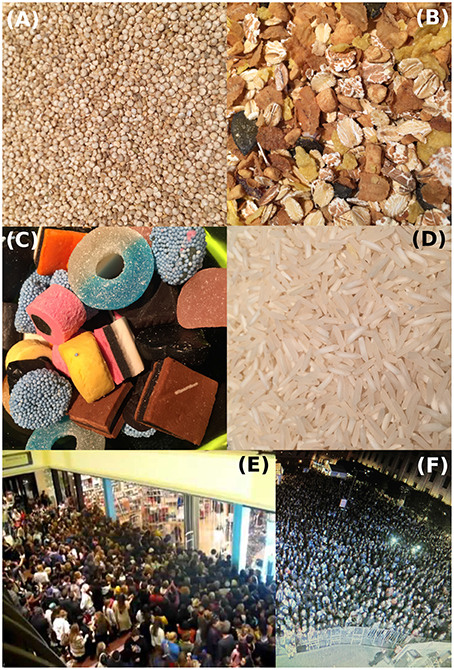
Figure 1. Common examples of non-human granular media including (A) quinoa, (B) muesli, (C) mixed candy, and (D) rice, compared to high-density human crowds at (E) a Black Friday sales event and (F) an outdoor concert. Similarities with the former inspires an analysis of the latter. This collection of images represents a cross-section of the various geometries, heterogeneities, and interactions that fall within the purview of granular media methods.

In the sections that follow, we describe how to implement the basic steps of eigenmode analysis and effectively interpret the results for high-density human crowds. While the method itself is quite general, we demonstrate the protocol through the example of an asocial model for high-density human collective behavior. In step-by-step fashion, we specifically emphasize practical tips for working with data, whether it be numerically simulated or empirically collected.

2. Methods

We divide the methods section into two subsections. The first subsection describes a physical model for asocial human collective behavior in high-density crowds. This model is motivated by previous work and provides a specific means for simulating individual human trajectories [23, 24]. The second subsection details an analysis protocol that takes trajectory data as input, and converts this information into a quantitative description of emergent collective behavior. This protocol may be broadly applied to trajectory data from sources other than the asocial model.

2.1. A Physical Model to Study High-Density Human Collective Behavior

To quantitatively model human collective behavior, we take a Newtonian force-based approach to generate complex emergent phenomena [25–29]. While systems studied within this “active matter” framework are generally non-equilibrium, the resulting phenomenology is often reminiscent of behaviors analyzed in the fields of statistical mechanics, granular materials, and fluid dynamics. As such, there is a rich tradition of concepts from these fields intermixing [13–15].

2.1.1. Equations of Asocial Model

We specifically investigate human collective motion in high-density crowds. We therefore simplify the richness of human life to four forces, numerically simulate the resulting equations of motion, and investigate the emergent collective behavior. Referring to these simplified humans as Self-Propelled Particles (SPPs), we assume they are all interested in going toward a single point of interest, ${P}$. This point could be the front of a concert stage, the police line at a protest, or the exit of a stadium. While these activities have clear social differences, their commonality is in the accumulation of a large densely-packed crowd drawn by a common attraction. Each SPP indexed by i can now be described as a disk with radius r₀ positioned at a point ${\overrightarrow{r}}_i(t)$ and subject to: a pairwise soft-body repulsive collision force

$\begin{array}{cc}{\overrightarrow{F}}_i^{\text{repulsion}}=ϵ{\displaystyle \sum _{j\ne i}^N{\left(1-r_{i,j}/2r_0\right)}^{3/2}}{\widehat{r}}_{i,j},& (1)\end{array}$

which is non-zero only when the distance between two particles $|{\overrightarrow{r}}_i-{\overrightarrow{r}}_j|=\left|d_{ij}{\widehat{r}}_{i,j}\right|=d_{ij}<2r_0$ [23, 24]; a self-propulsion force

$\begin{array}{cc}{\overrightarrow{F}}_i^{\text{propulsion}}=\mu (v_0{\widehat{p}}_i-{\overrightarrow{v}}_i),& (2)\end{array}$

where v₀ is a constant preferred speed, ${\overrightarrow{v}}_i$ is the current velocity of the i^th SPP, and ${\widehat{p}}_i$ is a unit vector pointing from each particle's center to the common point of interest ${P}$; a randomly fluctuating force with components

$\begin{array}{cc}{\overrightarrow{F}}_i^{\text{noise}}={\overrightarrow{\eta }}_i,& (3)\end{array}$

drawn from a zero-mean Gaussian distribution and standard deviation σ defined by the correlation function $\langle {\eta }_{i,\lambda }(t){\eta }_{i,\kappa }(t^{\prime })\rangle =2{\mu }^{-1}{\sigma }^2{\delta }_{\lambda \kappa }\delta (t-t^{\prime })$, ensuring noise is spatially and temporally decorrelated; and finally, a wall collision force used to construct a confining simulation environment

$\begin{array}{cc}{\overrightarrow{F}}_i^{\text{wall}}=ϵ{\displaystyle \sum _{\text{walls}}{\left(1-r_{i,w}/r_0\right)}^{3/2}\widehat{w},}& (4)\end{array}$

which is pointed along each wall's outward normal direction ŵ and non-zero when the distance of the SPP from the wall r_i,w < r₀. While other repulsion forces have been used in similar models of human collective behavior [30–32], the functional form of ${\overrightarrow{F}}_i^{\text{repulsion}}$ and ${\overrightarrow{F}}_i^{\text{wall}}$ used here comes from treating SPP collisions as a Hertzian contact mechanics problem involving frictionless elastic spherical bodies [24, 33, 34]. Summing the forces from Equations (1) to (4), we find the evolution of each SPPs dynamics is driven by

$\begin{array}{cc}{\ddot{\overrightarrow{r}}}_i(t)={\overrightarrow{F}}_i^{\text{repulsion}}+{\overrightarrow{F}}_i^{\text{propulsion}}+{\overrightarrow{F}}_i^{\text{noise}}+{\overrightarrow{F}}_i^{\text{wall}}={\overrightarrow{F}}_i^{\text{total}},& (5)\end{array}$

where the relative magnitudes of individual force terms can be tuned through the scalar coefficients ϵ and μ. Because Equation (5) lacks any terms that reflect social interaction, we refer to it as an asocial model for high-density human collective behavior [23].

2.1.2. Numerical Implementation

Simulations take place in a rectangular room with wall length L ≫ r₀ centered at the origin (0, 0). The attraction point ${P}$ is placed at the center of the right wall at (L/2, 0) and N SPPs are seeded at random initial positions with zero initial speed and acceleration. At every integration time-step we compute the total force acting on individual SPPs at their current positions ${\overrightarrow{r}}_i(t)$ and evolve their trajectories according to Equation (5) (Figure 2). This calculation is performed numerically with the Newton-Stomer-Verlet algorithm, which finds the next position using the current velocity ${\stackrel{.}{\overrightarrow{r}}}_i(t)={\overrightarrow{v}}_i(t)$ and current acceleration ${\ddot{\overrightarrow{r}}}_i(t)={\overrightarrow{F}}_i^{\text{total}}(t)$ according to:

$\begin{array}{cc}{\overrightarrow{r}}_i(t+\Delta T)={\overrightarrow{r}}_i(t)+{\overrightarrow{v}}_i(t)\Delta T+\frac{1}{2}{\overrightarrow{F}}_i^{\text{total}}(t){(\Delta T)}^2.& (6)\end{array}$

The next acceleration ${\ddot{\overrightarrow{r}}}_i(t+\Delta T)={\overrightarrow{F}}_i^{\text{total}}(t+\Delta T)$ is then calculated at this new position, so that the next velocity can be determined by an average of the current and next accelerations:

$\begin{array}{cc}{\overrightarrow{v}}_i(t+\Delta T)={\overrightarrow{v}}_i(t)+\frac{{\overrightarrow{F}}_i^{\text{total}}(t)+{\overrightarrow{F}}_i^{\text{total}}(t+\Delta T)}{2}\Delta T.& (7)\end{array}$

Looping this sequence of calculations produces trajectories for each of the N SPPs (Figure 2). In Equations (6) and (7) the parameter Δt defines the integration step, which should be small enough to ensure smooth trajectories, but large enough to achieve reasonable computation times. Here, we run our simulations for t = 3,000τ units of time with ΔT = τ/10 = 0.10, yielding a total of 30,000 integration steps. Every 10 time steps we record each SPPs position ${\overrightarrow{r}}_i(t)$ as well as the pressure due to radial contact forces

$\begin{array}{cc}{P}_i(t)=\frac{1}{2\pi r_0}\left[{\overrightarrow{F}}_i^{\text{repulsion}}+{\overrightarrow{F}}_i^{\text{wall}}\right]·{\widehat{r}}_i,& (8)\end{array}$

where the dot product is with the unit normal vector centered on the i^th SPP. We consistently find transient motion dominates the first ≈ 50τ of the simulation resulting in far-from-equilibrium effects (Figures 2, 3, linear path segments). By 300τ the SPPs have aggregated near ${P}$ and formed a stable, dense, disordered aggregate with ${\overrightarrow{F}}_i^{\text{propulsion}}$ acting similar to an external field confining the SPPs. Within the aggregate, collision and noise forces are responsible for position fluctuations, causing each particle to move randomly around its average position (Figure 3 inset, densely accumulated trajectory data near the point of interest ${P}$ denoted by ⋆).

FIGURE 2

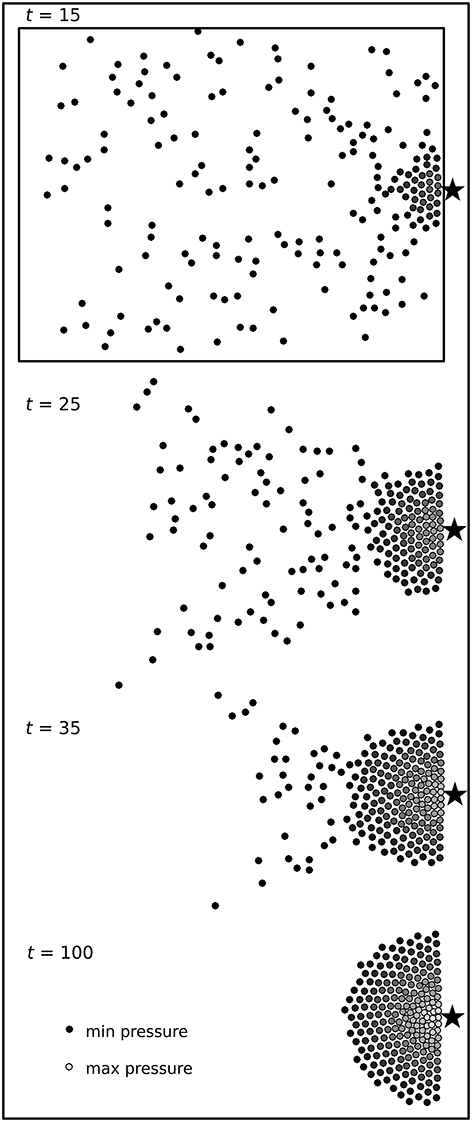
Figure 2. Four screenshots of a typical simulation run for our asocial model of high-density human crowds. Here, we see N = 200 SPPs aggregating near a point of interest ${P}$ denoted by ⋆, which is located at the right-most edge of a simulation box. SPPs self-organize into a dense and disordered aggregate, where shading is assigned according to the radial pressure at time t. The rectangular outline for t = 15 gives an impressionistic sense of the simulation box; the true border is taller and somewhat wider.

FIGURE 3

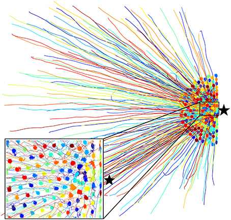
Figure 3. Trajectories r_i(t) for N = 200 SPPs in a typical simulation run of the asocial model for high-density human crowds. After a transient period (radial lines toward ⋆), the SPPs reach a stable state where they randomly oscillate about their average position (inset, dense squiggles). Each SPP is given a different color to more easily distinguish it from its neighbors.

2.1.3. Model Parameters and Time Scales

Setting model parameters in terms of the fundamental simulation unit length ℓ and unit time τ allows us to maintain careful control over the relative force and time scales while not explicitly committing to dimensionful units such as meters or seconds. As such, we simulate N = 200 SPPs of radius r₀ = ℓ/2 in a region of size L = 50ℓ. These choices ensure the simulation box size L is larger than the typical aggregated SPP group size $~\ell \sqrt{N}$. We also set the SPP preferred speed v₀ = ℓ/τ, the random force standard deviation σ = ℓ/τ², and the force scale coefficients ϵ = 25ℓ/τ², μ = τ⁻¹ [24]. For our analysis, we run 10 independent simulations of the dynamics with this set of parameters and random initial conditions.

Setting r₀ = ℓ/2 means that in the absence of any other interactions a SPP would move a distance equal to its diameter in the time τ. This choice approximates relaxed pedestrian motion if we were to have τ equal to one second [30].

The coefficient μ relates to an exponential relaxation time for the self-propulsion force, which can be seen by solving for free acceleration of a SPP. Specifically, dv/dt = μ(v₀ − v) has a solution v(t) = v₀[1 − exp(−μt)] when v(t = 0) = 0. This expression shows that an unobstructed SPP will exponentially approach its preferred speed v₀ with a timescale μ⁻¹.

Both SPP-SPP and SPP-wall collisions are subject to a Hertzian repulsion force directed normally to the surface of contact with a magnitude set by the coefficient ϵ. These forces are non-singular, making them numerically stable and easy to simulate, which is particularly useful for studies of jammed soft granular matter [34]. In the context of human crowds, Equations (1) and (4) greatly simplify collisional interactions, while still capturing the fact that people can be partially compressed with a rising non-linearity as the stresses increase. Here, ϵ is a constant for all SPPs equal to 25ℓ/τ², which guarantees the collision force scale is substantially larger than the self-propulsion force scale $\mu v_0=\ell /{\tau }^2$.

To ensure collisions and random force fluctuations contribute roughly equally to the SPPs dynamics, the collision time scale τ_coll and the random force time scale τ_noise must be comparable. In our asocial model, the random collision time scale τ_coll = 1/(2r₀v₀n) ≈ (π/4)τ is given by the mean-free path ${(2r_{0}n)}^{-1}\approx (\pi /2)r_0$ divided by the preferred speed v₀. The average crowd density $n\approx N/\pi {(\sqrt{N}{r}_0)}^2$ is estimated by noting the steady-state configuration of SPPs is roughly a half-circle with radius $\sqrt{N}{r}_0$ surrounding ${P}$. The noise time scale τ_noise can be found by calculating the amount of time required for random fluctuations to change the correlation function $\langle {\left[v_i({\tau }_{\text{noise}})-v_i(0)\right]}^2\rangle =2{\mu }^{-1}{\sigma }^2{\tau }_{\text{noise}}$ by an amount equal to $v_0^2$. Hence, ${\tau }_{\text{noise}}=\mu v_0^2/2{\sigma }^2$. Because the unit speed v₀ is fixed by the fundamental simulation units, and μ is set by the self-propulsion relaxation time, we simply let σ = ℓ/τ² to satisfy τ_noise = τ/2 ≈ τ_coll at steady-state.

2.2. Analysis Protocol of Trajectory Data

In section 2.1, we outlined a physical model for generating trajectory data of simulated human crowds using SPPs. In this section, we provide a step-by-step protocol for analyzing trajectory data using mode analysis as a means for predicting emergent collective motion. While we demonstrate the protocol with simulated data from the asocial model, our analysis can be applied equally well to other active jammed systems. As such, we cast our discussion in terms of “agents,” which could be either SPPs, actual humans being studied with cameras, or other examples of high-density active matter under consideration.

2.2.1. Step 1: Calculate the Displacement Covariance Matrix Components C_ij to Estimate the Ground-Truth Correlation Matrix C_p

Each of the trajectories ${\overrightarrow{r}}_i(t)=\langle x_i(t),y_i(t)\rangle$ provide spatially resolved position data on the i = 1, …, N agents at discrete time points t. From these trajectories, we want to determine the displacement correlation matrix C_p, which contains information about pair-wise correlated motion arising from the local interactions and the resulting collective motion. Ideally, this matrix is a statistical quantity averaged over all realizations of the underlying system. In practice, there are a limited number of computational runs or experimental measurements available. Thus, we calculate the covariance matrix [C_ij], whose components C_ij converge to the ground-truth correlation matrix C_p in the t → ∞ limit. These components are

$\begin{array}{cc}{C}_{ij}=\langle [{\overrightarrow{r}}_i(t)-\langle {\overrightarrow{r}}_i\rangle ]·[{\overrightarrow{r}}_j(t)-\langle {\overrightarrow{r}}_j\rangle ]\rangle ,& (9)\end{array}$

where time averages 〈⋯〉 are calculated for each realization of the underlying random process over a statistically-independent sub-sampling of the time series data. Conventionally, this is the equivalence between time and ensemble averaging. Critical Note 1: While Equation (9) is standard notation in the literature, it obscures the fact that there are actually two sets of covariance matrix components to calculate: one each for the x and y directions. A more transparent representation would be

$\begin{array}{cc}\begin{array}{l}{C}_{ij}^x=\langle [x_i(t)-\langle x_i\rangle ]·[x_j(t)-\langle x_j\rangle ]\rangle \text{and}\\ C_{ij}^y=\langle [y_i(t)-\langle y_i\rangle ]·[y_j(t)-\langle y_j\rangle ]\rangle .\end{array}& (10)\end{array}$

However, the cumbersome nature of these expressions tends to favor the aesthetics and compactness of Equation (9). Critical Note 2: Time-averaging calls for a judicial eye that balances two competing demands: sub-sampling in time should be spaced out to reduce effects from auto-correlated motion, while simultaneously leaving a sufficient number of statistically-independent “snap-shots” of the system for the components of the covariance matrix [C_ij] to converge to the correlation matrix C_p. A straight-forward convergence criteria is to ensure the ratio 2N/N_t < 1.5, where N_t is the number of independent snap-shots [16]. Critical Note 3: Because mode analysis depends on the eigenvalues and eigenmodes of [C_ij], the quality of time averaging can be tested by examining how the eigenvalue spectrum converges as a function of the temporal sampling rate [16]. Specifically, the spectrum should be insensitive to the sampling rate; comparing spectra generated at different sampling rates will indicate whether a specific value is in this regime. Critical Note 4: Many physical models can be treated with scaling analysis to determine a minimal estimate for the time scale of auto-correlated motion. In the asocial model described in section 2.1, noise and repulsive collision forces dissipate auto-correlation. Thus, the trajectory data should be sub-sampled at temporal intervals spaced out longer than τ_noise and τ_coll. Critical Note 5: In some circumstances such as an external perturbation or sudden motion, the agents being studied can undergo rearrangements in position that change the internal structure of which agents are in contact with each other. When this occurs, the covariance matrix components C_ij must be recalculated from post-rearrangement trajectory data and convergence of [C_ij] → C_p must be rechecked.

Example: Determining appropriate temporal sub-sampling of asocial model. For the parameter values described above, we find the simulation reaches steady state after ≈ 50τ. We generously discard the first 300τ to eliminate far-from-equilibrium transients leaving 2, 700τ of trajectory data for each SPP. Because τ_noise = τ/2 ≈ τ_coll, then τ/2 is the minimal estimate for temporal sub-sampling. From this baseline, we check convergence of the eigenvalue spectrum for intervals longer than τ/2, and find a temporal sub-sampling of 10τ is adequate. We are then left with N_t = (2, 700τ)/(10τ) = 270 statistically-independent snap-shots of the system to use when calculating temporal averages in Equation (9), which is consistient with the 2N/N_t = 1.48 < 1.5 criteria.

2.2.2. Step 2: Calculate the Eigenmodes and Eigenvalue Spectrum

Having calculated a displacement covariance matrix [C_ij] that approximates the ground-truth correlation matrix C_p, we can now use standard numerical techniques to compute the eigenvalues λ_m and their corresponding eigenmodes ${\overrightarrow{e}}_m$. The index m = 1, …, N runs over all agents under consideration. Often, the terminology “eigenmode” is simply shortened to “mode,” which is a callback to the field's roots in analyzing harmonic vibrational motion. Critical Note 1: Sorting the eigenvalues in decreasing order and plotting as a function of index m gives the spectrum of the covariance matrix, which in the t → ∞ limit converges to the spectrum of the correlation matrix. Critical Note 2: As in the previous step, notational conventions obscure the fact that there are two sets of eigenvalues and eigenmodes. Specifically, both x and y directions have their own eigenvalues ${\lambda }_m^x$ and ${\lambda }_m^y$ for a total of 2N eigenvalues with two distinct spectra. Likewise, each eigenmode is a two-dimensional displacement vector field. For example, the m = 1 eigenmode is more transparently expressed as $\langle {\overrightarrow{e}}_1^x,{\overrightarrow{e}}_1^y\rangle$, with ${\overrightarrow{e}}_1^x=\left\{e_{1,1}^x,e_{1,2}^x,\dots ,e_{1,N}^x\right\}=\left\{e_{1,j}^x\right\}$ and ${\overrightarrow{e}}_1^y=\left\{e_{1,1}^y,e_{1,2}^y,\dots ,e_{1,N}^y\right\}=\left\{e_{1,j}^y\right\}$. These 2N components indexed by j = 1, …, N are the m = 1 eigenmode values in the x and y directions for each of the j agents. Critical Note 3: The eigenmodes are typically normalized such that $\sum _{j=1}^N{e}_{m,j}^x=1$, $\sum _{j=1}^N{e}_{m,j}^y=1$, and the norm $\sum _{j=1}^N|{\overrightarrow{e}}_{m,j}{|}^2=2$. Critical Note 4: Within a linear approximation, the eigenmodes express relative magnitude and directions for harmonic oscillation of the agents about their mean positions. The eigenvalues relate to the corresponding excitation energies of these modes. Trajectory data $\overrightarrow{r}(t)$ can then be decomposed into a linear combination of these modes with a collection of 2N time-dependent coefficients. As the non-linearity and non-equilibrium nature of the system asserts itself, these approximations breakdown.

2.2.3. Step 3: Find and Remove Rattlers

Plotting low-m eigenmodes as two-dimensional displacement fields frequently reveals a small number of agents N_r ≪ N that represent a disproportionately large amount of the overall motion. This phenomenon is well-known to arise in both experimental and simulated jammed systems, where such agents are called “rattlers.” While most often studied in colloidal suspensions and vibrated/sheared granular packings, rattlers get their name because they are surrounded by highly-constrained neighbors that create a rigid cage enclosing enough space for the rattler to freely move about [22, 35]. This under-constrained motion is therefore a consequence of local structure. Because (i) rattlers tend not to participate in global collective motion and (ii) the location of rattlers is impossible to predict a priori, we must identify them a posteriori, remove the N_r rattlers from consideration, and recompute Equation (9) with the subset of N − N_r agents. A threshold identification criteria is useful for systematically finding rattlers. In particular, for each mode m we check for agents with index j whose individual displacement

$\begin{array}{cc}|{\overrightarrow{e}}_{m,j}|={\left[{(e_{m,j}^x)}^2+{(e_{m,j}^y)}^2\right]}^{1/2}& (11)\end{array}$

is greater than the mode's average displacement

$\begin{array}{cc}\langle |{\overrightarrow{e}}_m|\rangle =\frac{1}{N}{\displaystyle \sum _{j=1}^N{\left[{(e_{m,j}^x)}^2+{(e_{m,j}^y)}^2\right]}^{1/2}}& (12)\end{array}$

plus ξ_r times the mode's standard deviation

$\begin{array}{cc}\begin{array}{l}{\sigma }_m={\left[{({\sigma }_m^x)}^2+{({\sigma }_m^y)}^2\right]}^{1/2}\\ ={\left[{\displaystyle \sum _{j=1}^N\frac{{[e_{m,j}^x-\langle |e_m^x|\rangle ]}^2+{[e_{m,j}^y-\langle |e_m^y|\rangle ]}^2}{N-1}}\right]}^{1/2}.\end{array}& (13)\end{array}$

More succinctly, rattlers are defined as agents with index j with $\left|{\overrightarrow{e}}_{m,j}\right|\ge \langle |{\overrightarrow{e}}_m|\rangle +{\xi }_r{\sigma }_m$, for a given threshold value ξ_r. Once identified, these N_r agents can be removed from further consideration. Critical Note 1: The removal of rattlers ensures low-m modes reflect genuine collective motion of the system instead of the free vibrations of under-constrained agents. Critical Note 2: Selection of an appropriate threshold should be done by testing multiple values of ξ_r and examining how the fraction N_r/N varies. If the threshold is too high, then the eigenmodes will continue to be dominated by the uncorrelated motion of rattlers. If the value is too low, then the analysis risks under-sampling the calculation of C_ij and no collective motion will be detected. As a general heuristic, the value of N_r arising from ξ_r should be the minimum value that removes anomalous uncorrelated motion from the low-m modes. No single value of N_r/N will be appropriate for all circumstances, and the selection of ξ_r should be given due consideration. In the next step we provide further useful information to aid in the choice of ξ_r and illustrate the procedure in the case of our simulation data.

2.2.4. Step 4: Re-calculate the Eigenmodes and Eigenvalue Spectrum without Rattlers

Having provisionally identified the N_r rattlers in step 3, we repeat steps 1 and 2 to re-calculate the eigenmodes and eigenvalue spectrum from [C_ij] with the remaining N − N_r agents. When examining the new modes and spectra produced by step 2, we generally find the first attempt at removing rattlers is insufficient and steps 1 through 3 should be performed as an iterative process to optimally determine ξ_r. Critical Note 1: Concretely, this strategy starts with an initial guess for the threshold ξ_r, and determines a final value by qualitatively and quantitatively checking how ξ_r affects the eigenmodes and eigenvalue spectrum. The goal is to find a value of ξ_r that filters rattlers from the overall collective motion in low-m eigenmodes. Critical Note 2: While iterating, it's useful to: (i) visually confirm whether the eigenmode plots are being affected by under-constrained motions, and (ii) confirm the eigenvalue spectra retain their basic shape. This information is essential for making an informed decision on the next threshold value to test. Critical Note 3: A reasonable initial guess for the rattler threshold is to set ξ_r = 1 with the expectation that the final value will be larger.

Example: Iteratively selecting ξ_r. Working with trajectory data generated by the asocial model, we perform steps 1 through 4 of the analysis protocol and test various values for the rattler threshold ξ_r (Figure 4). In this instance, we seek to find and remove rattlers from the first 10 modes by examining values of ξ_r ranging from 1 to 6. As prescribed in the protocol, we calculate and re-calculate the eigenvalue spectrum eliminating provisionally identified rattlers from consideration. These comparisons show the general form of the eigenvalue spectra remain largely unchanged for a range of ξ_r, and the number of rattlers decreases substantially for ξ_r > 1 (Figure 4D). In addition to examining the spectra and N_r/N ratio, we also examine plots of the modes before (Figure 5, red) and after (Figure 5, blue) rattlers are removed with ξ_r = 4. With this choice for ξ_r, rattlers are less than 1% of the total number of agents, and we find in two separate simulation runs that large irregular vector arrows in low-m modes are no longer present. In this case, we have successfully filtered rattler motion out from the overall collective behavior, leaving a set of N − N_r eigenmodes and eigenvalues for downstream analysis.

FIGURE 4

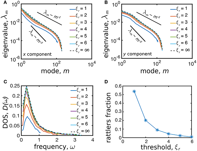
Figure 4. The eigenvalue spectrum of the displacement correlation matrix before removing the rattlers (dashed black line, threshold for removal is infinitely large) and after removing the rattlers using different values of the threshold ξ_r (solid colored lines, threshold for removal is finite) for the (A) x and (B) y components. (C) The basic shape of the DOS is conserved for different values of the threshold ξ_r. (D) The fraction of rattlers monotonically decreases as the threshold value ξ_r increases.

FIGURE 5

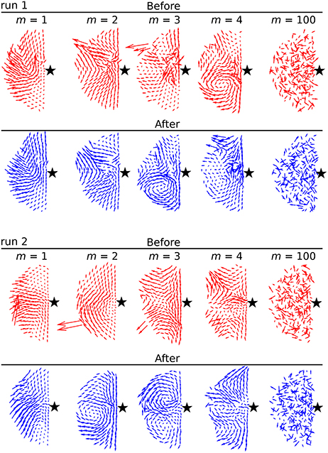
Figure 5. Visualization of five eigenmodes for two independent simulation runs before (red) and after (blue) removing the rattlers with a threshold choice of ξ_r = 4. Removing rattlers affects the first few eigenmodes by filtering out large irregularly-oriented vectors, but has little effect at higher m.

2.2.5. (Optional) Step 5: Alternative Heuristic Method for Finding Rattlers

We briefly mention an alternative method for finding rattlers. This heuristic involves the computation of each agent's positional auto-correlation time Δt* from the trajectory data ${\overrightarrow{r}}_i(t)=\langle x_i(t),y_i(t)\rangle$ and the auto-correlation functions

$\begin{array}{cc}\begin{array}{l}{\chi }_i^x(\Delta t)=\frac{1}{T}{\displaystyle \sum _{t=1}^{T-\Delta t}}\left[x_i(t)-\langle x_i\rangle \right]\times \left[x_i(t+\Delta t)-\langle x_i\rangle \right],\text{and}\\ {\chi }_i^y(\Delta t)=\frac{1}{T}{\displaystyle \sum _{t=1}^{T-\Delta t}}\left[y_i(t)-\langle y_i\rangle \right]\times \left[y_i(t+\Delta t)-\langle y_i\rangle \right].\end{array}& (14)\end{array}$

Here, the normalizations are over all T time steps, and the averaging 〈⋯〉 is calculated for individual agents. We seek minimal time delays Δt^x and Δt^y such that ${\chi }_i^x(\Delta t^x)={\chi }_i^y(\Delta t^y)=0$, which average to the auto-correlation time Δt* = (Δt^x + Δt^y)/2. Because rattlers are free to move within their local region, they are generally not influenced by their neighbors and we expect these agents to have the highest auto-correlation times. Critical Note 1: The auto-correlation times are independently calculated for each of the i agents even though Δt* does not have an explicit index i. Critical Note 2: Auto-correlation measurements can have non-trivial behavior that requires individualized assessment. Some cases of note include: when multiple time delays where χ_i = 0 are found, we simply take the smallest value of Δt; when there are no time delays with χ_i = 0, it may be appropriate to fit a smooth function and extrapolate the delay time that χ_i intersects zero; when the auto-correlation functions are noisy and it appears that Δt as-defined is erroneous, it may be appropriate to smooth the data and infer a revised value of Δt. Critical Note 3: While the heuristic approach for finding rattlers has the advantage of being rapidly calculated directly from raw trajectory data, it does not have the same degree of accuracy as the threshold identification method. This cost-benefit assessment suggests the heuristic approach may find its most effective applications in real-time inference of crowd diagnostics.

Example: Testing heuristic identification of rattlers. Step 3 of the mode analysis protocol identifies rattlers based on each agent's positional fluctuations within a given mode. Here, we consider a side-by-side comparison for three simulation runs showing how a threshold of ξ_r = 4 compares with the distribution of auto-correlation times. Evidently, the agreement is considerable (Figure 6, overlapping red circles and dark squares, especially in runs 1 and 3), though certainly not perfect (Figure 6, non-overlapping red circles and dark squares, especially run 2). When an abundance of data and analysis time is available, the threshold approach is clearly preferable for its accuracy. However, in circumstances that limit the availability of data or when analysis is needed in near-real-time, the heuristic may be preferable.

FIGURE 6

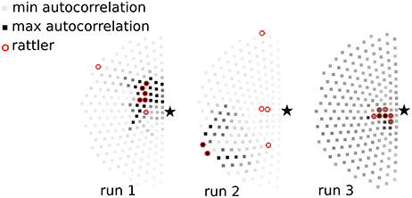
Figure 6. Heuristic identification of rattlers through their auto-correlation time Δt*. Each SPP is shown as a square and shaded according to Δt*. In runs 1 and 3 the SPPs with the highest auto-correlation time are also identified as rattlers by the threshold method (red circles, ξ_r = 4). In run 2 this heuristic is less successful at identifying rattlers near the center of the aggregate.

2.2.6. (Optional) Step 6: Calculate the Density of States (DOS)

In mode analysis, the Density of States (DOS) D(ω²) is used to quantify the probability of having a certain number of excitable oscillations at frequency ω within a given energy range ~ ω². This concept is well-defined at equilibrium, but more tenuous in non-equilibrium systems such as the asocial model considered here. The value of using a DOS analysis is that it sheds light on how a perturbation will transfer energy into various modes, as long as the perturbation itself does not substantially disrupt the organization of agents that defines the modal structure. To calculate D(ω²), we note the eigenvalues are related to harmonic frequencies by ${\lambda }_m={\omega }_m^{-2}$. Since oscillation energy is proportional to the frequency squared, D(ω²) is essentially a histogram of the inverse-eigenvalues. Critical Note 1: The DOS conveys information about the rigidity of a solid; when there are many low-energy modes, the system is “soft” and will appear unstable to excitations. Here again, we mention the caveat that “low-energy modes” in the asocial model are a linearized approximation of the true response. Critical Note 2: A useful conceptual touchstone is the Debye law for regular lattices wherein the DOS is often expressed as the density of frequencies ω as opposed to energies ω². In d dimensions, the Debye law is D(ω) ~ ω^d−1.

Example: Interpreting eigenvalue spectra through a DOS lens. We previously analyzed the eigenvalue spectra to examine their dependence on the rattler threshold ξ_r. To provide additional context for these plots, we can explicitly plot the DOS (Figure 4D) to reveal the distribution of low-frequency excitations. These measurements provide a potential target of opportunity for theoretical predictions.

2.2.7. (Optional) Step 7: Find Soft Spots

When studying jammed granular materials, certain regions are often found to be partially under-constrained resulting in the presence of “soft spots” that are more likely to undergo large structural rearrangements when the system is perturbed [19]. In the context of analyzing dense human crowds, soft spots localize the people undergoing the largest displacements. The agents in these soft spots are known as “bucklers” [22], and they can be identified with a thresholding process similar to the one used to find rattlers. In this case, we seek the N_s non-rattler agents indexed by j from the collection of low-m modes with $\left|{\overrightarrow{e}}_{m,j}\right|\ge \langle |{\overrightarrow{e}}_m|\rangle +{\xi }_S{\sigma }_m$, where each term is defined as in Equations (11)–(13), and ξ_S is a yet-to-be-determined threshold for finding agents in soft spots. We also seek the N_D non-rattler agents indexed by i whose dynamics in 〈x, y〉 obey

$\begin{array}{cc}\langle |{\overrightarrow{r}}_i(t)-\langle {\overrightarrow{r}}_i\rangle |\rangle \ge {\displaystyle \sum _{i=1}^{N-N_r}\frac{\langle |{\overrightarrow{r}}_i(t)-\langle {\overrightarrow{r}}_i\rangle |\rangle }{(N-N_r)}}+{\xi }_D{\sigma }_D,& (15)\end{array}$

which identifies the agents whose displacement fluctuations are greater than the average by an amount equal to ξ_Dσ_D. Here, σ_D is the standard deviation of displacements in 〈x, y〉 averaged over the non-rattler population, and ξ_D is another yet-to-be-determined threshold. Bucklers can now be defined as the set of agents identified by both thresholds when ξ_S and ξ_D are chosen to maximize the overlap between the two sets. This condition is quantified by the normalized agreement function (NAF)

$\begin{array}{cc}\text{NAF}=\left[1-\frac{N_S}{N-N_r}\right]·\left[1-\frac{N_D}{N-N_r}\right]\frac{|S\cap D|}{|S\cup D|},& (16)\end{array}$

where S and D are the set of agents identified by ξ_S and ξ_D, respectively. Critical Note 1: The bracketed prefactors in Equation (16) are weighting functions that dampen the measure of overlap if either set oversamples the total population. Critical Note 2: Bucklers tend to cluster in well-defined areas. In the asocial model, one of these areas is the perimeter of the SPP aggregate where the edge agents are trivially under-constrained and can be ignored as an artifact. Critical Note 3: An analogous thresholding can be performed with the SPP confinement pressure defined in Equation (8) and used in place of the average displacement fluctuations from Equation 15. This is useful if pressure fluctuations are hypothesized to correlate with “softness” in a specific study.

Example: Calculating thresholds and visualizing soft spots. For each of the simulation runs, we identified which agents had significant displacement fluctuations, pressure fluctuations, and mode fluctuations when the prescribed thresholds ranged from ξ_D, ξ_P = 1 to 7 and ξ_S = 1 to 5. Examining the simple overlap between these sets without normalization prefactors (Figure 7, top row), indicates a range of threshold values with substantial overlap within the sets, particularly for low threshold values. This agreement is spurious due to an oversampling of the total population at low thresholds. Using appropriate weighting functions from Equation (16) (Figure 7, middle row) to normalize the agreement function reveals a more well-defined range of thresholds for ξ_D and ξ_S wherein ≈ 10% of the agents are in soft spots (Figure 7, bottom row). The agreement is maximized for ξ_S = 2.5 and ξ_D = 4.5, and we take these values to definitively identify soft spots for this example system. Other thresholds may be more appropriate for different sources of trajectory data. We also find essentially no correlation between the confinement pressure fluctuations and softness, indicating these quantities are essentially independent in the asocial model. To visualize soft spots, we plot the dense aggregate of agents and highlight individuals that were identified as having mode fluctuations above the ξ_S = 2.5 level in at least one of the first 10 modes (Figure 8). Color coding the first 10 modes for three simulation runs and recalling that agents on the perimeter are trivially under-constrained, we see soft spots are consistently localized near the core of the aggregate. This implies a high-probability of structural rearrangements will occur in this area when the system is excited.

FIGURE 7

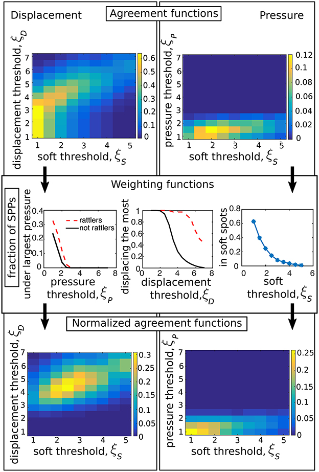
Figure 7. The agreement functions for the correlation between being in a soft spot (S), undergoing large pressure (P), and large displacement (D) before (top) and after (bottom) the normalization by the weighting functions (center) that measure the size of the sets S, P, D. Arrows indicate the logical procedure followed to obtain the normalized agreement functions.

FIGURE 8

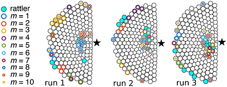
Figure 8. Identification of soft spots for three independent simulation runs. Each SPP is shown as a disk and the star (⋆) represents the point of interest ${P}$. Superimposing data for the first 10 modes shows that soft spots appear in multiple modes in the same general area near the core of the aggregate. Apparent soft spots along the periphery are artifacts due to under-constrained edge effects.

2.2.8. (Optional) Step 8: Find Soft Modes

In the harmonic theory of crystals, eigenmodes of the displacement correlation matrix [C_ij] fully characterize a linear response of the system to perturbations [36]. When excited, each of these “normal modes” requires an energy whose cost is inversely proportional to their corresponding eigenvalue. While useful for studying jammed granular systems, this linearized theoretical framework can break down if harmonicity or energy equipartition are violated. In such circumstances, an equivalence between the dynamical matrix C_p and displacement correlation matrix [C_ij] becomes tenuous and deserving of further consideration. However, information about the system's structural stability, coherent collective motion, and localized kinematics may nevertheless be conveyed through “soft modes.” These modes are the eigenmodes corresponding to the highest eigenvalues of [C_ij], which in turn, are the lowest excitation energies of the linearized theory [17–19].

To determine which modes of [C_ij] calculated in steps 1–4 are soft, we compare the agent's eigenvalue spectrum to a spectrum arising from uncorrelated motion. Specifically, we generate a set of N − N_r random displacements with zero mean and standard deviation σ_RM. This standard deviation of the random displacements is chosen to be equal to the standard deviation of the agent's displacements around their equilibrium positions. We then calculate the covariance matrix and eigenvalue spectrum for this Random Matrix Model (RM_σ). Comparing spectra, we now have a threshold condition: when the eigenvalues from steps 1 to 4 are greater than the eigenvalues from RM_σ, we identify the associated modes as soft modes because they relate to correlated motion; when the eigenvalues from steps 1 to 4 are less than or equal to the eigenvalues from RM_σ, we identify the associated modes as essentially random uncorrelated motion. Critical Note 1: When comparing spectra, all data should be averaged over all independent simulation runs. Critical Note 2: This approach has roots in principal component analysis and studies of jammed granular systems, where soft modes indicate preferential directions of relaxation in the system [16]. In terms of human crowds, we interpret soft modes as the preferential directions of collective motion because these modes feature low excitation energies, suggesting their emergence is likely to occur when a dense crowd is slightly perturbed.

Example: Using soft modes to concretely define “low-m” modes. By calculating the RM_σ spectrum and superimposing eigenvalues from simulated human crowds, we see there are up to m = 6 soft modes in both the x and y directions (Figure 9A, modes above dashed line). For practical purposes, we can now use the RM_σ threshold to quantitatively define these low-m modes as the system's soft modes. Recalling that eigenvalues and oscillation frequencies are related by ${\lambda }_m={\omega }_m^{-2}$, we see in the DOS that correlated motions of soft modes correspond to a low-frequency Bosonic peak typically associated with long-range collective motion near the jamming transition (Figure 9B) [37–39]. This observation suggests the system is not mechanically stable, and that small perturbations could excite soft modes resulting in major structural rearrangements. In terms of human crowds, this would explain from a physical point of view why sudden collective motion can spontaneously emerge at high density. To visualize these collective motions, we plot the displacement vector fields for the first six soft modes from a single run (Figure 9C). We see they indeed carry a high degree of spatial correlation at low-m that rapidly diminishes with increasing mode number. In this example the spectra are averaged over 10 independent runs and rattlers have been removed.

FIGURE 9

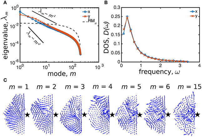
Figure 9. Eigenmode analysis of asocial model for high-density human crowds. (A) Eigenvalue spectrum λ_m of the displacement correlation matrix exhibits scaling properties between ${\lambda }_m~m^{-1}$ and ~ m⁻² (black solid lines). Eigenmodes up to m = 6 in both x (blue) and y (orange) directions are larger than the random matrix model (RM_σ, dashed line), thus they are named “soft modes” and describe correlated motion. (B) The DOS exhibits a Bosonic peak in both the x and y components, indicating mechanical instability. (C) Soft mode vector fields for run 1 (m = 1 to 6) are more spatially correlated than a mode below RM_σ (m = 15).

3. Results

The previous section described an asocial model for simulating high-density human crowds and provided a step-by-step protocol for identifying several different types of emergent collective motion. Here, we draw inspiration from a variety of physical concepts to further interpret the information conveyed by mode analysis and its specific meaning for human collective behavior.

3.1. The m = 1 mode Is a Pseudo-Goldstone Mode

Symmetry plays a critical role for nearly all fields of modern physics. In condensed matter, the spontaneous breaking of continuous symmetries is often associated with the emergence of long-range low-energy excitations known as Goldstone modes [40–42]. For example, studies of flocking in active systems have found the interaction of self-propulsion and directional alignment breaks global rotation invariance, leading to rapid collective directional changes known as the “Goldstone mode of the flock” [43–46]. In other examples, where continuous symmetries are instead explicitly broken by exogenous factors, we find pseudo-Goldstone modes, which require a small but finite energy for excitation. With these considerations in mind, we note the asocial model involves a propulsion force aligned to a specific point of interest ${P}$ that explicitly breaks 〈x, y〉 translational symmetry (Equation 2). We therefore predict a low-energy long-range pseudo-Goldstone mode to be a fundamental collective excitation of the asocial model.

One way to check if one or more of our system's modes is a pseudo-Goldstone mode is to examine whether the polarization correlation length is system-spanning [46]. Practically, this is accomplished by calculating the mean polarization vector $\overrightarrow{\Phi }(m)=N^{-1}\sum _{i=1}^N{\overrightarrow{e}}_m^i/\left|{\overrightarrow{e}}_m^i\right|$ and measuring the correlation function of each mode's fluctuations $C_m(d)={\langle [{\overrightarrow{e}}_m^i-\overrightarrow{\Phi }(m)]·[{\overrightarrow{e}}_m^j-\overrightarrow{\Phi }(m)]\rangle }_{d_{ij}=d}$ about this average value [46]. In this last expression, the average is over all particles i and j whose pairwise distance d_ij is equal to the distance d. We then define the correlation length l_c(m) as the minimum distance at which C_m(l_c) = 0. Plotting C_m(d) for a few modes shows that most have a relatively short correlation length, while the m = 1 mode extends across the entire system (Figure 10). This system-wide excitation is at the lowest possible mode number, which in linear mode theory corresponds to the lowest possible excitation energy. Thus, these two pieces of evidence combine to strongly implicate the m = 1 mode as a pseudo-Goldstone mode. Because its origins can be traced to a broken continuous symmetry, this long-range highly correlated collective motion is an intrinsic effect of densely aggregated agents.

FIGURE 10

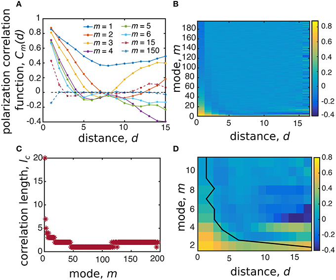
Figure 10. The polarization correlation length identifies the m = 1 mode as a pseudo-Goldstone mode. (A) The correlation function C_m(d) for the mode polarization fluctuations plotted against distance between particles d decays rapidly for modes m > 1, which can be seen in a heat map (B) for all modes. (C) The correlation length for all modes defined as the distance ℓ_c where C_m(ℓ_c) = 0. (D) Examining the first 12 modes as a heat map and superimposing the correlation length number illustrates where C_m(d) = 0.

In our asocial model, the m = 1 mode is a collective motion that slides up-and-down along the right-most edge of the simulation box (Figure 9C). In real-world circumstances this means the most easily-excitable mode would result in a large number of people being suddenly displaced together, possibly toward a wall, concert stage, or some other barrier. Such a situation has been widely observed in conjunction with the emergence of shock waves and density waves during “crowd turbulence” [12, 47]. Since its origins can be traced to the general principle of symmetry breaking, this type of long-range collective motion can be expected as a latent excitation arising in a wide range of circumstances with the potential for causing crowd crush casualties [48].

3.2. Topological Defect Density Drives Disorder in the Modes

If broken symmetries and pseudo-Goldstone modes can explain the m = 1 long-range collective motion, then what is the most useful way to understand the remaining m > 1 modes? Remarkably, and somewhat surprisingly, topological principles provide useful insights. Two modes are considered topologically equivalent if their vector fields can be continuously deformed to match one another, and as such, the difference in excitation energy will become arbitrarily small as their alignment converges [42]. However, the introduction of a topological defect, such as vortices in superfluids, magnetic flux tubes in superconductors and edge-dislocations in liquid crystals, prevent convergence and drive a persistent non-zero energetic difference. To check whether topological defects play a meaningful role in explaining the structure of eigenmode m, we calculate the winding number charge $q_i={(2\pi )}^{-1}{\oint }_{\ell }\overrightarrow{\nabla }\theta ·{\overrightarrow{d\ell }}_i$ for each non-edge agent i using a path ℓ_i that loops around i's nearest-neighbors. Here, $\overrightarrow{\nabla \theta }$ measures the change in orientation between each agent's eigenmode vector along the loop. This measure is 0 when there are no topological defects, +1 if there is a vortex centered on the agent, or −1 if there is an anti-vortex centered on the agent. We can therefore identify each agent as coinciding with a topological defect depending on whether the local vector field makes a vortex with positive or negative charge q_i. Qualitatively examining q_i for a handful of different modes, it is clear that there are a number of topological defects, especially for m > 1 (Figure 11A). Recognizing that the rotation of the mode's vector field around these defects will reduce the correlation length, we sum the total absolute defect charge $Q_{\text{abs}}(m)=\sum _{i=1}^N\left|q_i\right|$ for each mode (Figure 11B) and estimate the expected correlation length. Assuming n defects are randomly distributed among N agents in a half disk of radius R and area πR²/2, the spatial distribution of defects can be expressed by a Poisson process of intensity ρ_q:

$\begin{array}{cc}P(n,R)=\frac{{\left[{\rho }_q\pi R^2\right]}^n}{2n!}{e}^{-{\rho }_q\pi R^2/2},& (17)\end{array}$

where ρ_q = Q_abs/N is the defect density. The probability to find the first defect closest to the disk's origin at a distance greater than R is equal to $F(>R)=P(\mathrm{\text{no point within R}})=exp\left[-{\rho }_q\pi R^2/2\right].$ Differentiating with respect to R and being careful with the sign of F(> R), we find the probability f(R) for the first neighbor at a distance R is $f(R)=\pi {\rho }_{q}R{e}^{-{\rho }_q\pi R^2/2}.$ Thus, the average nearest-neighbor distance 〈R〉 between any two points in the semi-disc is:

$\begin{array}{cc}\begin{array}{l}\langle R\rangle ={\displaystyle {\int }_0^{\infty }R}f(R)\text{d}R,\\ ={\displaystyle {\int }_0^{\infty }\pi }{\rho }_q{R}^2{e}^{-{\rho }_q\pi R^2/2}\text{d}R,\\ =-{\left[R{e}^{-{\rho }_q\pi R^2/2}\right]}_0^{\infty }+{\displaystyle {\int }_0^{\infty }{e}^{-{\rho }_q\pi R^2/2}}\text{d}R,\\ =\sqrt{\frac{2}{\pi {\rho }_q}}{\displaystyle {\int }_0^{\infty }{e}^{-t^2}}\text{d}t,\\ =\frac{1}{\sqrt{2{\rho }_q}},\end{array}& (18)\end{array}$

which is the average distance between two topological defects at density ρ_q. To connect 〈R〉 with the polarization fluctuation correlation length, we notice that if two neighboring defects are both positive or both negative, the mode's vector field cannot change direction in the space separating them, therefore l_c = 〈R〉. However, if two neighboring defects have opposite signs, the vector field must change sign and l_c ≈ 〈R〉/2. Therefore, on average we have

$\begin{array}{cc}\langle l_c(m)\rangle =\frac{1}{2}\langle R\rangle +\frac{1}{2}\frac{\langle R\rangle }{2}=\frac{3}{4}\sqrt{\frac{N}{2Q_{abs}(m)}}.& (19)\end{array}$

This last expression is a parameter-free theoretical prediction that readily agrees with our numerical computations (Figure 11C), suggesting that disordered features of modes m > 1 arise from topological defects distributed throughout the system. For m < 50 (Figure 11B), we interpret this result as indicating that modes cannot be continuously deformed into lower energy collective excitations, while for m > 50 a maximum disorder is reached due to a saturation in defect density.

FIGURE 11

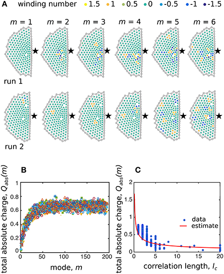
Figure 11. Topological defects drive disorder in m > 1 modes. (A) Winding number charge q_i for the soft modes of two independent simulation runs. Each SPP is colored according to its winding number and topological defects are centered on SPPs with q_i ≠ 0. In both simulation runs the number of topological defects increases with mode number. (B) The total absolute charge Q_abs plotted against mode number m for 10 independent simulation runs shows the number of defects increases with increasing mode number. (C) Scatterplot of the total absolute charge Q_abs vs. correlation length l_c for each mode of the 10 independent runs (circles) compared to the parameter-free predicted estimate from our geometric argument (line).

3.3. Collective Motion has Microscopic Structural Origins

Understanding collective motion in high-density crowds is motivated by an impetus to predict and prevent human disaster. Thus far, we have successfully linked individual trajectories to emergent collective motion through mode analysis. While the analysis provides insights such as the existence of soft spots and psuedo-Goldstone excitations, the specific locations and orientations of these phenomena depend on trajectory data. Consequently, these details can only be unlocked through an after the fact analysis, as opposed to the more-desirable goal of assessing risk in real-time. Nevertheless, it should still be possible to perform real-time risk assessment given that these collective motions ultimately depend on the microscopic self-organized structure of the crowd. The question remains: how do we make such an inference?

When we examine the structure of high-density crowds, it clearly deviates from the well-known hexagonal packing of 2D hard disks under uniform conditions. In the asocial model, these irregularities arise from a pressure gradient, which is calculated by averaging Equation (8) as a function of distance from the point of interest ${P}$ (Figure 12A). The structural irregularities created by this pressure gradient can be quantified by similarly computing the average number of interacting neighbors, also as a function of distance from ${P}$. Within the bulk of the crowd, this value is typically equal to six (Figure 12B, black line), which would be expected for homogeneous packing, while increasing to seven near ${P}$ due to the higher pressure (Figure 12B, dashed black line). If we now filter our averaging to examine just the bucklers within soft spots, we see the average number of interacting neighbors is measurably higher, suggesting that the local coordination number contains a signature of these potentially high-risk locations (Figure 12B, solid red line). Examining specific runs and comparing the local coordination number (Figure 12C) to the location of bucklers in soft spots (Figure 12D), we find a broad consistency between these two measures. The critical point here is that the coordination number can be extracted from a single “snap-shot” of the crowd, whereas soft spots are identified through the full machinery of mode analysis. Even if the mapping is not perfectly one-to-one, coordination number may provide a valuable correlate for predicting the location of high-risk areas before collective motions become excited.

FIGURE 12

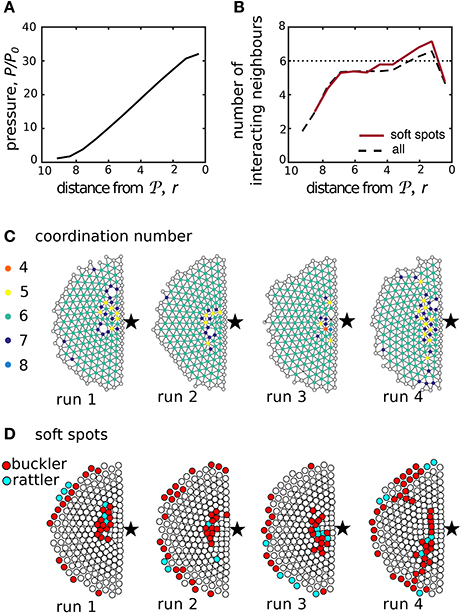
Figure 12. Local coordination number correlates with soft spots. (A) The average radial pressure normalized by $P_0=\mu v_0{(2\pi r_0)}^{-1}$ reveals a gradient within the aggregate. This pressure drives deviations (B) from homogenous hexagonal packing as measured by the average number of interacting neighbors at a distance r from the point of interest ${P}$. Hexagonal close packings of hard disks have six interacting neighbors, which is added as a dashed line for reference. (C) The local coordination number, shown here for 4 runs, can be computed from a snap shot of the system. Comparison with (D) shows the coordination number strongly correlates with the location of soft spots, which are found through more lengthy computations involving the identification of aggregated bucklers (red).

If soft spots are indeed a consequence of local structure, the mechanistic connection remains to be identified and understood. Therefore, we measure the two particle radial structure factor $g(d)={\left[(N-N_r)(N-N_r-1)\right]}^{-1}\sum _{i=1}^{N-N_r}\sum _{j\ne i}^{N-N_r}\delta (d-d_{ij})$, which quantifies the radial distribution of distances between neighboring agents. Unlike globally averaged properties, g(d) provides information about the local structure [38]. For the asocial model, it reveals that the overall structure has clear short range order (Figure 13, peaks for d < 3) but no periodic long range order (Figure 13, generally smooth distribution for d > 3). We see the position of the first peak centered at d = 0.8 suggests that, on average, the agents slightly overlap due to the self-propulsion forces. When we filter our measurement and reexamine g(d) strictly for the bucklers in soft spots, the data shows a new sub-peak around 0.5 ≲ d ≲ 0.8, while a second more prominent peak shifts to d ≈ 0.9. This seems to suggest the structure within a soft spot is asymmetrically squeezed with nearest-neighbors somewhat closer than average in one direction, presumably in the direction of ${P}$, while also somewhat further away than average from other neighbors. As a result, this irregular structure provides a microscopic mechanism for bucklers to easily displace when perturbed.

FIGURE 13

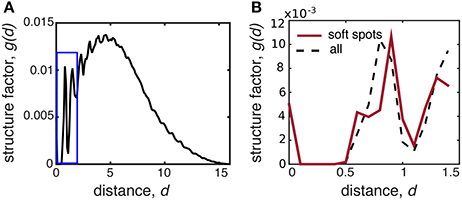
Figure 13. The structure factor g(d) helps explain why local coordination predicts location of soft spots. (A) The structure factor g(d) shows short range order (peaks for d ≲ 3), but generally no long-range order. (B) Zooming in on the blue boxed region from (A), we see differences in local structure between bucklers in soft spots (red solid line) and the averaged aggregate (black dashed line). All data is generating by averaging over 10 independent simulation runs.

In terms of high-density human crowds, motion can be thought of as the superposition of the most easily excited modes. When motion occurs, our analysis predicts that people in soft spots would be the ones displacing the most. We therefore interpret soft spots as posing the highest risk for tripping and subsequent trampling, especially if activated by a sudden and unexpected external perturbation. Qualitatively, this phenomenon has been observed in a number of crowd disasters, when sudden unexpected movements of the crowd cause individuals to trip and fall, resulting in injury or death due to trampling or compressive asphyxia [12, 48, 49]. Furthermore, the observation that these areas can be heuristically detected through heterogeneity in the local coordination number provides a potential target for real-time prediction and prevention.

3.4. The “Participation Ratio” and “Effective Coordination Number” Do Not Measure Collectiveness in the Asocial Model

While we were able to successfully co-localize soft spots with the local coordination number, there are two additional metrics we tested that were found to provide insufficiently detailed information. Nevertheless, because these metrics are more widely used to study densely-packed jammed systems, we provide an overview of our findings so that others may have our null results as a reference. Our main finding with these metrics is that they seem to detect a difference between high- and low-m modes with a transition around m ≈ 50, similar to the transition found when measuring the density of topological defects (Figure 11B). However, this says little about soft modes, the eigenvalue spectrum, the DOS, or auto-correlation length. Any deeper significance for active matter systems apparently requires further analysis.

A standard measure for the collectiveness of a mode is given by the participation ratio PR(m), which quantifies how many agents in the system move when a given mode is excited. In the literature there are several definitions of this metric [16, 21], and while we tested them all, we present results when PR(m) is calculated as

$\begin{array}{cc}\text{PR}(m)=\frac{{\left({\displaystyle {\sum }_{i=1}^N{\left|{\overrightarrow{e}}_m^i\right|}^2}\right)}^2}{N{{\displaystyle {\sum }_{i=1}^N\left|{\overrightarrow{e}}_m^i\right|}}^4},& (20)\end{array}$

which, respectively, takes values between 0 and 1 for fully localized and fully extended collective motion [21]. Plotting the participation ratio against mode number m provides a signature of the system and gives an overview of the collective nature of modes. In our case, we find the participation ratio for soft modes is lower than the random matrix RM_σ, and increases toward 1/2 with mode number m (Figure 14A). This occurs because the typical length of the displacements on the high-m modes are highly similar while their direction is random. Conversely, soft mode displacements are more variable in length but more correlated in direction. This seems to suggest that in the framework considered here, the participation ratio is not an appropriate measure for detecting collective behavior.

FIGURE 14

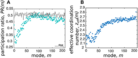
Figure 14. While consistent with our general findings, not all measures of structure explain collective motion. (A) The participation ratio PR(m) initially decreases as a function of mode number, but after m ~ 6 increases toward the random case (dotted line). (B) The effective coordination number z_eff(m) shows the lowest modes are under-constrained.

Another commonly used metric to characterize modes is the effective coordination number [21]:

$\begin{array}{cc}{z}_{\text{eff}}(m)=\frac{\left({\displaystyle {\sum }_{i=1}^N{z}_i|{\overrightarrow{e}}_i^m{|}^2}\right)}{{\displaystyle {\sum }_{i=1}^N|{\overrightarrow{e}}_i^m{|}^2}}-3,& (21)\end{array}$

where z_i is the number of neighbors interacting with the i^th agent defined as d_ij < 2r₀, and −3 is to remove degrees of freedom associated with global 2D rotational/translational symmetries. This expression calculates the average number of constraints per agent in each mode, weighted by their displacement on that mode. In jammed solids, its value depends on the amount of compression and affects the frequency ω of modes [21]. Here, we cannot precisely relate the eigenvalues to the energy of the system, therefore z_eff(m) simply helps identify over- or under-constrained modes. In particular, rigid stability requires z_eff(m) ≥ 3; in light of our results (Figure 14B), the system appears generally non-rigid.

4. Discussion

With an eye toward understanding, predicting, and preventing tragedies at mass gatherings, we view our main results as revealing mechanisms for the emergence of potentially dangerous collective motion. By first identifying these principles and outlining a quantitative framework for measuring their existence, we are now in position to test their real-world applicability using video data of concerts, pilgrimages, and sporting events. This next step is a straight-forward empirical data collection process, given the current availability of low-cost high-definition digital cameras and inexpensive cloud-computing resources for rapid image analysis. The only remaining obstacle, therefore, is to develop computer vision algorithms that robustly and automatically track individual trajectories in footage of high-density crowds. While this image analysis challenge is open-ended, it may be sufficient for our purposes to simply study coarse-grained fields of view that average motion over regional domains encompassing several people.

If the methods outlined here prove to be broadly predictive in describing high-density human collective motion when no disasters occur, then they will become a valuable starting point for developing conceptually new strategies that enhance safety at mass gatherings. In the long term, we hope our results will lead to practical tools for real-time monitoring and predictive diagnostics at mass events. We also note that while the techniques described here are motivated by human crowds, they provide an analytical framework for extracting key insights from other real-world problems such as the characterization of biological tissues, the dynamics of migrating cancer cells, animal collective motion, real-time material characterization, and self-monitoring industrial assembly-lines.

Author Contributions

AB and JS contributed equally to this work, and approved it for publication.

Funding

This work was independently funded. Open-access fees were partially provided by the Harvard Open-Access Publishing Equity (HOPE) Fund.

Conflict of Interest Statement

The authors declare that the research was conducted in the absence of any commercial or financial relationships that could be construed as a potential conflict of interest.

The reviewer AK declared a shared affiliation, with no collaboration, with one of the author JS, to the handling Editor.

Acknowledgments

The authors thank R. Sanchez and M. Smith for their inspirational contributions.

References

1. Holland JH. Complexity: A Very Short Introduction. Oxford: Oxford University Press (2014).

Google Scholar

2. Thaler RH, Sunstein CR. Nudge: Improving Decisions About Health, Wealth, and Happiness. Westminster: Penguin Books (2009).

Google Scholar

3. Thaler RH. Misbehaving: The Making of Behavioral Economics. New York, NY: W. W. Norton and Company (2016).

4. Hausman DM, Welch B. Debate: to nudge or not to nudge. J Polit Philos. (2010) 18:123–36. doi: 10.1111/j.1467-9760.2009.00351.x

CrossRef Full Text | Google Scholar

5. King R, Churchill EF, Tan C. Designing with Data: Improving User Experience with A/B Testing. Sebastopol, CA: O'Reilly Media (2017).

6. Kohavi R, Thomke S. The surprising power of online experiments. Harvard Bus Rev. (2017) 5:74–82. https://hbr.org/2017/09/the-surprising-power-of-online-experiments

7. Aven T. On the meaning of a black swan in a risk context. Safety Sci. (2013) 57:44–51. doi: 10.1016/j.ssci.2013.01.016

CrossRef Full Text | Google Scholar

8. Taleb NN. The Black Swan: The Impact of the Highly Improbable. Random House Trade Paperbacks (2010).

9. Milsten AM, Maguire BJ, Bissell RA, Seaman KG. Mass-gathering medical care: a review of the literature. Prehosp Disast Med. (2002) 17:151–62. doi: 10.1017/S1049023X00000388

PubMed Abstract | CrossRef Full Text | Google Scholar

10. Carley S, Mackway-Jones K, Donnan S. Major incidents in Britain over the past 28 years: The case for the centralised reporting of major incidents. J Epidemiol Commun Health (1998) 52:392–8. doi: 10.1136/jech.52.6.392

PubMed Abstract | CrossRef Full Text | Google Scholar

11. Wagner U, Fälker A, Wenzel V. Fatal incidents by crowd crush during mass events:(Un) preventable phenomenon. Anaesthesist Der. (2013) 62:39–46. doi: 10.1007/s00101-012-2124-z

PubMed Abstract | CrossRef Full Text | Google Scholar

12. Helbing D, Johansson A, Al-Abideen HZ. Dynamics of crowd disasters: an empirical study. Phys Rev E (2007) 75:046109. doi: 10.1103/PhysRevE.75.046109

PubMed Abstract | CrossRef Full Text | Google Scholar

13. Helbing D, Johansson A, Mathiesen J, Jensen MH, Hansen A. Analytical approach to continuous and intermittent bottleneck flows. Phys Rev Lett. (2006) 97:168001. doi: 10.1103/PhysRevLett.97.168001

PubMed Abstract | CrossRef Full Text | Google Scholar

14. Cristiani E, Piccoli B, Tosin A. Multiscale modeling of granular flows with application to crowd dynamics. Multiscale Model Sim. (2011) 9:155–82. doi: 10.1137/100797515

CrossRef Full Text | Google Scholar

15. Faure S, Maury B. Crowd motion from the granular standpoint. Math Mod Meth Appl S (2015) 25:463–93. doi: 10.1142/S0218202515400035

CrossRef Full Text | Google Scholar

16. Henkes S, Brito C, Dauchot O. Extracting vibrational modes from fluctuations: a pedagogical discussion. Soft Matter (2012) 8:6092–109. doi: 10.1039/c2sm07445a

CrossRef Full Text | Google Scholar

17. Brito C, Dauchot O, Biroli G, Bouchaud JP. Elementary excitation modes in a granular glass above jamming. Soft Matter (2010) 6:3013–22. doi: 10.1039/c001360a

CrossRef Full Text | Google Scholar

18. Ashton DJ, Garrahan JP. Relationship between vibrations and dynamical heterogeneity in a model glass former: extended soft modes but local relaxation. Eur Phys J E (2009) 30:303–7. doi: 10.1140/epje/i2009-10531-6

PubMed Abstract | CrossRef Full Text | Google Scholar

19. Manning ML, Liu AJ. Vibrational modes identify soft spots in a sheared disordered packing. Phys Rev Lett. (2011) 107:108302. doi: 10.1103/PhysRevLett.107.108302

PubMed Abstract | CrossRef Full Text | Google Scholar

20. Henkes S, Fily Y, Marchetti MC. Active jamming: self-propelled soft particles at high density. Phys Rev E (2011) 84:040301. doi: 10.1103/PhysRevE.84.040301

PubMed Abstract | CrossRef Full Text | Google Scholar

21. Xu N, Vitelli V, Liu A, Nagel S. Anharmonic and quasi-localized vibrations in jammed solids: modes for mechanical failure. Europhys Lett. (2010) 90:56001. doi: 10.1209/0295-5075/90/56001

CrossRef Full Text | Google Scholar

22. Charbonneau P, Corwin EI, Parisi G, Zamponi F. Jamming criticality revealed by removing localized buckling excitations. Phys Rev Lett. (2015) 114:125504. doi: 10.1103/PhysRevLett.114.125504

PubMed Abstract | CrossRef Full Text | Google Scholar

23. Bottinelli A, Sumpter DTJ, Silverberg JL. Emergent structural mechanisms for high-density collective motion inspired by human crowds. Phys Rev Lett. (2016) 117:228301. doi: 10.1103/PhysRevLett.117.228301

PubMed Abstract | CrossRef Full Text | Google Scholar

24. Silverberg JL, Bierbaum M, Sethna JP, Cohen I. Collective motion of humans in mosh and circle pits at heavy metal concerts. Phys Rev Lett. (2013) 110:228701. doi: 10.1103/PhysRevLett.110.228701

PubMed Abstract | CrossRef Full Text | Google Scholar

25. Vicsek T, Zafeiris A. Collective motion. Phys Rep. (2012) 517:71–140. doi: 10.1016/j.physrep.2012.03.004

CrossRef Full Text | Google Scholar

26. Sumpter DJ. Collective Animal Behavior. Princeton, NJ: Princeton University Press (2010).

Google Scholar

27. Helbing D, Molnar P. Social force model for pedestrian dynamics. Phys Rev E. (1995) 51:4282. doi: 10.1103/PhysRevE.51.4282

PubMed Abstract | CrossRef Full Text | Google Scholar

28. Helbing D. A mathematical model for the behavior of pedestrians. Behav Sci. (1991) 36:298–310. doi: 10.1002/bs.3830360405

CrossRef Full Text | Google Scholar

29. Vivek S, Yanni D, Yunker PJ, Silverberg JL. Anticipating and inoculating against hacks that exploit the emergent collective motion of autonomous vehicles. arXiv:170803791 (2017).

Google Scholar

30. Helbing D, Farkas I, Vicsek T. Simulating dynamical features of escape panic. Nature (2000) 407:487–90. doi: 10.1038/35035023

PubMed Abstract | CrossRef Full Text | Google Scholar

31. Moussaïd M, Helbing D, Theraulaz G. How simple rules determine pedestrian behavior and crowd disasters. Proc Natl Acad Sci USA. (2011) 108:6884–8. doi: 10.1073/pnas.1016507108

PubMed Abstract | CrossRef Full Text

32. Helbing D, Johansson A. Pedestrian, crowd, and evacuation dynamics. arXiv:13091609 (2013).

Google Scholar

33. Landau LD, Lifshitz E. Course of Theoretical Physics: Theory of Elasticity, Vol. 7. New York, NY: Elsevier (1986).

34. Van Hecke M. Jamming of soft particles: geometry, mechanics, scaling and isostaticity. J Phys Condens Matter (2009) 22:033101. doi: 10.1088/0953-8984/22/3/033101

CrossRef Full Text | Google Scholar

35. Majmudar T, Sperl M, Luding S, Behringer RP. Jamming transition in granular systems. Phys Rev Lett. (2007) 98:058001. doi: 10.1103/PhysRevLett.98.058001

PubMed Abstract | CrossRef Full Text | Google Scholar

36. Ashcroft NW, Mermin ND. Solid State Physics. Stamford, CT: Thomson Learning (1976).

Google Scholar

37. Wyart M, Nagel S, Witten T. Geometric origin of excess low-frequency vibrational modes in weakly connected amorphous solids. Europhys Lett. (2005) 72:486. doi: 10.1209/epl/i2005-10245-5

CrossRef Full Text | Google Scholar

38. Laird BB, Schober H. Localized low-frequency vibrational modes in a simple model glass. Phys Rev Lett. (1991) 66:636. doi: 10.1103/PhysRevLett.66.636

PubMed Abstract | CrossRef Full Text | Google Scholar

39. Silbert LE, Liu AJ, Nagel SR. Vibrations and diverging length scales near the unjamming transition. Phys Rev Lett. (2005) 95:098301. doi: 10.1103/PhysRevLett.95.098301

PubMed Abstract | CrossRef Full Text | Google Scholar

40. Nambu Y. Quasi-particles and gauge invariance in the theory of superconductivity. Phys Rev. (1960) 117:648. doi: 10.1103/PhysRev.117.648

CrossRef Full Text | Google Scholar

41. Goldstone J. Field theories with superconductor solutions. Il Nuovo Cimento (1961) 19:154–64.

Google Scholar

42. Sethna J. Statistical Mechanics: Entropy, Order Parameters, and Complexity. Oxford, UK: Oxford University Press (2006).

Google Scholar

43. Toner J, Tu Y, Ramaswamy S. Hydrodynamics and phases of flocks. Ann Phys. (2005) 318:170–244. doi: 10.1016/j.aop.2005.04.011

CrossRef Full Text | Google Scholar

44. Ramaswamy S. The mechanics and statistics of active matter. Annu Rev Condens Matter Phys. (2010) 1:323–45. doi: 10.1146/annurev-conmatphys-070909-104101

CrossRef Full Text | Google Scholar

45. Cavagna A, Cimarelli A, Giardina I, Parisi G, Santagati R, Stefanini F, et al. Scale-free correlations in starling flocks. Proc Natl Acad Sci USA (2010) 107:11865–70. doi: 10.1073/pnas.1005766107

PubMed Abstract | CrossRef Full Text | Google Scholar

46. Bialek W, Cavagna A, Giardina I, Mora T, Pohl O, Silvestri E, et al. Social interactions dominate speed control in poising natural flocks near criticality. Proc Natl Acad Sci USA (2014) 111:7212–7. doi: 10.1073/pnas.1324045111

PubMed Abstract | CrossRef Full Text | Google Scholar

47. Takatori S, Yan W, Brady J. Swim pressure: stress generation in active matter. Phys Rev Lett. (2014) 113:028103. doi: 10.1103/PhysRevLett.113.028103

PubMed Abstract | CrossRef Full Text | Google Scholar

48. Fruin JJ. The causes and prevention of crowd disasters. Eng Crowd Safety (1993) 1:10.

49. Krausz B, Bauckhage C. Loveparade 2010: automatic video analysis of a crowd disaster. Comput Vis Image Und. (2012) 116:307–19. doi: 10.1016/j.cviu.2011.08.006

CrossRef Full Text | Google Scholar