Uncertainty of Volatility Estimates from Heston Greeks

1. Introduction

Volatility of stock prices is a highly volatile time-process itself. This insight led to the introduction of volatility indices like the VIX (1993) and its off-springs, based on the work [1, 2], which make volatility a trademark in its own right subject to similar stochastic movements as stock prices. According to this view volatility seems to be responsible for several statistical properties of observed stock price processes. In particular, volatility clustering, i.e., large fluctuations are commonly followed by other large fluctuations and similarly for small changes [3]. Another feature is that, in clear contrast with price changes which show negligible autocorrelations, volatility autocorrelation is still significant for time lags longer than 1 year [3–8]. Additionally, there exists the so-called leverage effect, i.e., much shorter (few weeks) negative cross-correlation between current price change and future volatility [3, 9–11].

In stochastic volatility models, volatility is considered as a hidden process which can only be observed indirectly via its effect on stock price dynamics. Thus, in practice it has to be inferred from market data. In a previous paper [12], we have shown that daily stock returns in general provide only very limited information about volatility. Thus, there are intrinsic limits on how precisely volatility can be recovered from market data. Here, we consider a related question when recovering volatility from option price data. Instead of the fairly general treatment in Pfante and Bertschinger [12] we address in the present paper the question how much information the VIX, as very popular measure for implied volatility of the S&P 500, actually provide about volatility. More precisely, how much information about volatility is contained the constituents of the VIX, i.e., near- and next-term put and call options on the S&P 500 with more than 23 days and less than 37 days to expiration and non-vanishing bid. We tackle this question in terms of Fisher information. To this end, we choose Heston's stochastic volatility model [13] because the pricing formulae of the European Call and Put Options are analytically tractable in terms of Fourier transforms. Then, assuming that observed option prices are centered on the theoretical price provided by Heston's model perturbed by additive Gaussian noise we investigate the precision of volatility estimates. Since the VIX basket consist of a vast number of Call and Put options on the S&P 500 results from asymptotic statistics [14] apply: the maximum likelihood estimator is consistent, asymptotically efficient, and normally distributed and the variance is the inverse of the Fisher information. Hence, Fisher information quantifies the uncertainty of maximum likelihood volatility estimates—at least asymptotically—and relates them to the partial derivatives, i.e., the Greeks, of the Heston model. While the Fisher information is commonly used to access the precision of parameter estimates, to our knowledge, it has not been applied in the context of implied volatility estimation previously.

Overall, we find that in contrast to stock returns alone [12], that the options in the basket of the VIX provide substantial information about volatility making inferred volatility a precise estimator as long as volatilities are sufficiently high. The picture changes dramatically for very small volatilities because Vega, the derivative of the option price w.r.t. volatility and thereby the Fisher information, almost vanishes below a critical value of about 3%. This in turn leads to huge relative errors in small inferred volatilities. The VIX, being a variance swap on the average volatility over 30 days, is much more stable with a relative uncertainty never exceeding a few percent over the considered data set.

The paper is structured as follows: section 2 introduces Heston's model and associated pricing formulae. Further, we explain how the fractional fast Fourier transform allows an efficient computation of the Heston Greeks. In section 2.4 we state the formal definition and important properties of Fisher information. Section 3.1 illustrates how the Fisher information varies w.r.t. strike and maturity in the Heston model. Further, we discuss the role of Vega on the reliability of volatility estimation. Finally, in section 3.2 we compute the Fisher information for the volatility of the S&P 500 index as well as the VIX index.

2. Materials and Methods

2.1. Heston's Stochastic Volatility Model

Introducing Heston's model for pricing options we follow Rouah [15]. The Heston model assumes that the underlying stock price, S_t, follows a Black-Scholes-type stochastic process, but with a stochastic variance v_t that follows a Cox, Ingersoll, and Ross process. Hence, the Heston model is represented by the bivariate system of stochastic differential equations (SDEs)

$\begin{array}{l}d{S}_t=\mu S_{t}dt+\sqrt{v_t}{S}_{t}d{W}_{1,t}\\ d{v}_t=\kappa (\theta -v_t)dt+\sigma \sqrt{v_t}d{W}_{2,t}& (2.1)\end{array}$

with the instantaneous correlation dW_{1, t}dW_{2, t} = ρdt of the two Brownian motions. The parameters of the model are

drift of the stock                      μ

relaxation parameter                κ > 0

long-term mean of the variance θ > 0

leverage-effect parameter         ρ ∈ [0, 1]

volatility of the variance            σ > 0 .

Furthermore, the price at time t of a zero-coupon bond paying 1$ at maturity t + τ is

$\begin{array}{l}P(t,t+\tau )=e^{-\tau r}\end{array}$

with constant interest rate r. Neglecting volatility risk premium, change of measure yields the log-price x_t = log S_t and variance v_t

$\begin{array}{ll}d{x}_t& =\left(r-\frac{1}{2}{v}_t\right)dt+\sqrt{v_t}d{\tilde{W}}_{1,t}\\ d{v}_t& =\kappa (\theta -v_t)dt+\sigma \sqrt{v_t}d{\tilde{W}}_{2,t}\end{array}$

w.r.t. to the risk neutral measure ℚ, see Rouah [15] or Heston's original work [13] for a detailed derivation. If we include a continuous dividend yield q, the time drift of the log-price becomes r − q − 1/2v_t.

2.2. European Options

We present the price for a European call and put option in Heston's model in the formulation of Carr and Madan [16]. Henceforth, we abbreviate the log-price x_t = log S_t at time t simply by x and similarly the variance v_t at time t by v. We only consider the characteristic function f of the cumulative distribution $P^{\mathbb{Q}}(x_{t+\tau }>logK)$ w.r.t. the risk-neutral probability, that is,

$\begin{array}{l}{P}^{\mathbb{Q}}(x_{t+\tau }>k)=\frac{1}{2}+\frac{1}{\pi }{\displaystyle {\int }_0^{\infty }}\Re 𝔢\left[\frac{e^{-i\varphi k}f(\varphi ,x,v,\tau )}{i\varphi }\right]d\varphi .\end{array}$

with

$\begin{array}{l}f(\varphi ,x,v,\tau )=e^{(C(\varphi ,\tau )+D(\varphi ,\tau )v+i\varphi x)}\end{array}$

and the logarithmic strike k = log K. The little Heston Trap formulation [17] yields

$\begin{array}{l}C(\varphi ,\tau )=i(r-q)\varphi \tau +\frac{\kappa \theta }{{\sigma }^2}\left[(Q-d)\tau -2log\left(\frac{1-c{e}^{-d\tau }}{1-c}\right)\right]\\ D(\varphi ,\tau )=\frac{Q-d}{{\sigma }^2}\left(\frac{1-e^{-d\tau }}{1-c{e}^{-d\tau }}\right)\end{array}$

with

$\begin{array}{l}c=\frac{Q-d}{Q+d}\\ d=\sqrt{Q^2+{\sigma }^2(i\varphi +{\varphi }^2)}\\ Q=\kappa -i\rho \sigma \varphi .\end{array}$

We introduce

$\begin{array}{l}E(\epsilon ,x,v,r,\kappa ,\theta ,\rho ,\sigma ,k,\tau )\\ =\frac{e^{-\epsilon \sigma k}}{\pi }{\displaystyle {\int }_0^{\infty }\Re }e\left[e^{{}^{-ik\varphi }}\widehat{e}(\epsilon ,\varphi ,x,v,\tau )\right]d\varphi & (2.2)\end{array}$

with

$\begin{array}{l}ê(ϵ,\varphi ,x,v,\tau )=\frac{e^{-r\tau }f(\varphi -i(ϵ\alpha +1),x,v)}{{(ϵ\alpha )}^2+ϵ\alpha -{\varphi }^2+i\varphi (2ϵ\alpha +1)}.\end{array}$

where ϵ ∈ {1, −1} and α > 0 is a positive damping factor controlling the numerical stability of the integration. α can either be fixed or chosen according to an optimization scheme outlined in Carr and Madan [16]. We obtain the European call C(x, v, r, κ, θ, ρ, σ, k, τ) and put P(x, v, r, κ, θ, ρ, σ, k, τ) price, respectively, via

$\begin{array}{l}C(x,v,r,\kappa ,\theta ,\rho ,\sigma ,k,\tau )=E(1,x,v,r,\kappa ,\theta ,\rho ,\sigma ,k,\tau )\\ P(x,v,r,\kappa ,\theta ,\rho ,\sigma ,k,\tau )=E(-1,x,v,r,\kappa ,\theta ,\rho ,\sigma ,k,\tau ).& (2.3)\end{array}$

We refer to Carr and Madan [16] or the third chapter in Rouah's book [15] for a derivation of the formulae Equation (2.3). Furthermore, we have put-call parity, see Rouah [15],

$\begin{array}{r}P(x,v,r,\kappa ,\theta ,\rho ,\sigma ,k,\tau )=C(x,v,r,\kappa ,\theta ,\rho ,\sigma ,k,\tau )\\ +e^k{e}^{-r\tau }-e^x{e}^{-q\tau }.& (2.4)\end{array}$

The Heston Greeks in terms of the Carr-Madan formulation read

$\begin{array}{l}\frac{\partial }{\partial \gamma }E(ϵ,x,v,r,\kappa ,\theta ,\rho ,\sigma ,k,\tau )\\ =\frac{e^{-ϵ\alpha k}}{\pi }{\displaystyle {\int }_0^{\infty }\Re \mathfrak{e}}[e^{-ik\varphi }{\mathfrak{f}}_{\gamma }(\varphi -i(ϵ\alpha +1),x,v,\tau )\widehat{e}(ϵ,\varphi ,x,v,\tau )]d\varphi & (2.5)\end{array}$

where 𝔣_γ are different functions for $\gamma \in \left\{{\sigma }_0,\kappa ,\sqrt{\theta },\rho ,\sigma \right\}$ and ${\sigma }_0=\sqrt{v}$ denotes the volatility.

2.3. Fractional Fourier Transform

Since the call and put price in Equation (2.3) is expressed via a single Fourier integral we can apply a Fractional Fast Fourier Transform to achieve a simultaneous computation of the call and put prices Equation (2.3) for various strikes. We follow the outline in Rouah [15]. We approximate the Fourier integral in Equation (2.2) by Simpson's integration scheme over a truncated integration domain for ϕ, using N equidistant points

$\begin{array}{l}{\varphi }_j=j\eta \text{\hspace{1em} for }j=0,\dots ,N-1\end{array}$

where η is the increment. Simpson's rule approximates the integral Equation (2.5) as

$\begin{array}{l}\frac{\partial }{\partial \gamma }E(ϵ,x,v,r,\kappa ,\theta ,\rho ,\sigma ,k,\tau )\\ \approx \frac{e^{-ϵ\alpha k}\eta }{\pi }{\displaystyle \sum _{j=0}^{N-1}\Re \mathfrak{e}}[e^{i{\varphi }_{j}k}{\mathfrak{f}}_{\gamma }({\varphi }_j-i(ϵ\alpha +1),x,v,\tau )\widehat{e}(ϵ,{\varphi }_j,x,v,\tau )]w_j& (2.6)\end{array}$

with the weight w₀ = w_N−1 = 1/3, w_j = 4/3 iff j is odd and w_j = 2/3 otherwise. Since we are interested in strikes near the money the range for the log-strikes k needs to be centered on the log-price x. The strike range is, thus, discretized using N equidistant points

$\begin{array}{l}{k}_u=-b+u\lambda +x\text{\hspace{1em} for }u=0,\dots ,N-1\end{array}$

where λ is the increment and b = Nλ/2. This produces log-strikes over the range [log S − b, log S + b − λ]. For a log-strike on the grid k_u we can write the sum Equation (2.6) as

$\begin{array}{l}\frac{\partial }{\partial \gamma }E(k_u)\\ \approx \frac{e^{-ϵ\alpha k_u}\eta }{\pi }{\displaystyle \sum _{j=0}^{N-1}\Re \mathfrak{e}}[e^{i{\varphi }_j{k}_u}{\mathfrak{f}}_{\gamma }({\varphi }_j-i(ϵ\alpha +1),x,v,\tau )\widehat{e}(ϵ,{\varphi }_j,x,v,\tau )]w_j\\ =\frac{e^{-ϵ\alpha k_u}\eta }{\pi }{\displaystyle \sum _{j=0}^{N-1}\Re \mathfrak{e}}[e^{ij\eta (-b+u\lambda +x)}{\mathfrak{f}}_{\gamma }({\varphi }_j-i(ϵ\alpha +1),x,v,\tau )\\ \widehat{e}(ϵ,{\varphi }_j,x,v,\tau )]w_j\\ =\frac{e^{-ϵ\alpha k_u}\eta }{\pi }{\displaystyle \sum _{j=0}^{N-1}\Re \mathfrak{e}}[e^{i\eta \lambda uj}{e}^{i(b-x){\varphi }_j}{\mathfrak{f}}_{\gamma }({\varphi }_j-i(ϵ\alpha +1),x,v,\tau )\\ \widehat{e}(ϵ,{\varphi }_j,x,v,\tau )]w_j& (2.7)\end{array}$

for u = 1, …, N − 1. Applying a discrete Fast Fourier Transform (FFT) on Equation (2.7) imposes the restriction

$\begin{array}{rc}\lambda \eta =\frac{2\pi }{N}& (2.8)\end{array}$

on the choice of the increments λ and η which entails a trade off between the grid sizes. Hence, Chourdakis [18] introduced the Fractional Fast Fourier Transform (FRFT) to relax this important limitation of the discrete FFT. The term 2π/N in Equation (2.8) is replaced by a general term β and Equation (2.7) becomes

$\begin{array}{rc}{\widehat{x}}_u=E(k_u)\approx \frac{e^{-ϵ\alpha k_u}\eta }{\pi }{\displaystyle \sum _{j=0}^{N-1}}\Re 𝔢\left[e^{i\beta uj}{x}_j\right]& (2.9)\end{array}$

with

$\begin{array}{l}{x}_j=e^{i(b-x){\varphi }_j}{𝔣}_{\gamma }({\varphi }_j-i(ϵ\alpha +1),x,v,\tau )ê(ϵ,{\varphi }_j,x,v,\tau )w_j\\ j=1,\dots ,N-1.\end{array}$

The relationship between the grid sizes λ and η becomes λη = β. Thus, we can choose the grid size parameters η and λ freely. To implement the FRFT on the vector x = (x₀, …, x_N−1) we first define vectors

$\begin{array}{l}\mathbf{y}=\left({\left\{e^{-i\pi j^2\beta }{x}_j\right\}}_{j=0}^{N-1},{\left\{0\right\}}_{j=0}^{N-1}\right)\\ \mathbf{z}=\left({\left\{e^{i\pi j^2\beta }\right\}}_{j=0}^{N-1},{\left\{e^{i\pi {(N-j)}^2\beta }\right\}}_{j=0}^{N-1}\right).\end{array}$

Next, a discrete FFT of the vectors y and z yields $\widehat{\text{y}}=D(\text{y})$ and $\widehat{\text{z}}=D(\text{z})$ and we define the 2N dimensional vector

$\begin{array}{l}\widehat{\text{h}}=\widehat{\text{y}}\odot \widehat{\text{z}}={(y_j{z}_j)}_{j=0}^{2N-1}.\end{array}$

where ⊙ denotes pointwise multiplication.

Now, we apply the inverse FFT on $\widehat{\text{h}}$ and take the pointwise product of the result with the vector

$\begin{array}{l}e=\left({\left\{e^{-i\pi j^2\beta }\right\}}_{j=0}^{N-1},{\left\{0\right\}}_{j=0}^{N-1}\right)\end{array}$

to obtain

$\begin{array}{l}\widehat{\text{x}}=e\odot D^{-1}(\widehat{\text{h}})=e\odot D^{-1}(\widehat{\text{y}}\odot \widehat{\text{z}})=e\odot D^{-1}(D(\text{y})\odot D(\text{z})).\end{array}$

If we truncate the last N elements we obtain the desired vector x of Equation (2.9) with length N. Hence, the FRFT maps a vector of length N onto another vector of length N, even though it uses intermediate vectors of length 2N.

2.4. Fisher Information in Pricing Options

The outline on the Fisher information follows Cover and Thomas [19] and Ibragimov and Has'minskii [14]. We begin with a few definitions. Let $\left\{f(x;\Theta )\right\},\Theta =({\theta }_1,\dots ,{\theta }_m)\in {P}\subset {ℝ}^m$, denote an indexed family of densities $f:{X}\to {ℝ}_{\ge 0},\int f(x;\theta )dx=1$ for all $\Theta \in {P}$. Here ${P}$ is called the parameter set. The ij-th entry of the Fisher information matrix J(Θ) is defined by

$\begin{array}{l}J{(\Theta )}_{ij}=\int \frac{\partial }{\partial {\theta }_i}logf(x;\Theta )\frac{\partial }{\partial {\theta }_j}logf(x;\Theta )f(x;\Theta )dx\\ =𝔼\left[\frac{\partial }{\partial {\theta }_i}logf(x;\Theta )\frac{\partial }{\partial {\theta }_j}logf(x;\Theta )\right]\end{array}$

Fisher information has the following properties. First, as covariance matrix, the Fisher information matrix is positive semi-definite. Second, information is additive: the information yielded by two independent experiments is the sum of the information from each experiment separately:

$\begin{array}{l}{J}_{X,Y}(\Theta )=J_X(\Theta )+J_Y(\Theta )\end{array}$

Third, the Fisher information depends of the parametrization of the problem: suppose Θ and Λ are m-vectors which parametrize the estimation problem, and suppose Θ is a continuously differentiable function of Λ, then

$\begin{array}{rc}J(\Lambda )=D^{T}J(\Theta (\Lambda ))D& (2.10)\end{array}$

where the ij-th entry of the m × m Jacobian D is defined by D_ij = ∂θ_i/∂λ_j and D^T denotes the transpose of D.

The Fisher information matrix of a single option with price e is a way of measuring the amount of information that the observable option price e carries about the unknown parameters ${\sigma }_0,\kappa ,\sqrt{\theta },\rho ,\sigma$. Recall, σ₀ is the volatility, κ the relaxation parameter of the CIR process Equation (2.1), θ the long-term mean of the variance, σ the volatility of the diffusion process Equation (2.1), and ρ the leverage parameter, i.e., the instantaneous correlation between the two Brownian motions in Equation (2.1). While Heston's option price E(ϵ, x, v, r, κ, θ, ρ, σ, k, τ) is a function of the stated parameters, the observed price e might deviate from its theoretical value. Following standard practice in fitting the volatility smile, we consider the mean squared loss between the actually observed option price e and its theoretical value. In statistical terms, this corresponds to a noise model where the option price e is normally distributed around its theoretical mean value with variance $\widehat{v}$. The probability function for e, which is also the likelihood function for the parameter vector $\Theta =({\sigma }_0,\kappa ,\sqrt{\theta },\rho ,\sigma )$, is a function f(e; Θ); it is the probability mass (or probability density) of the random option price e conditional on the value of Θ. For a certain actual stock price S, strike K, and maturity τ we assume

$\begin{array}{l}f(e|\Theta )=\frac{1}{\sqrt{2\pi \widehat{v}}}exp\left(-\frac{{(e-E(ϵ,x,v,r,\kappa ,\theta ,\rho ,\sigma ,k,\tau ))}^2}{2\widehat{v}}\right)\end{array}$

where x = log S, k = log K, and $v={\sigma }_0^2$. We obtain the ij-th entry of the Fisher information matrix

$\begin{array}{rc}J{(\Theta )}_{ij}=\frac{1}{\widehat{v}}{\nabla }_{\Theta }E{({\nabla }_{\Theta }E)}^T& (2.11)\end{array}$

where

$\begin{array}{l}{\nabla }_{\Theta }E={\left(\frac{\partial }{\partial {\theta }_i}E(ϵ,x,v,r,\kappa ,\theta ,\rho ,\sigma ,k,\tau )\right)}_{i=1,\dots ,5}\end{array}$

is the gradient of the option price w.r.t. the parameters $({\theta }_1,\dots ,{\theta }_5)=({\sigma }_0,\kappa ,\sqrt{\theta },\rho ,\sigma )$.

Furthermore, we consider deviations of observed prices of options with different strikes and maturities from their respective theoretical prices as independent. Additivity of Fisher information yields

$\begin{array}{l}J(\Theta )=\frac{1}{\widehat{v}}{\displaystyle \sum _{\tau \in {T},k\in {K}}}{J}_{\tau ,k}(\Theta )\end{array}$

for simultaneously observed prices $\left\{E(ϵ,x,v,r,\kappa ,\theta ,\rho ,\sigma ,k,\tau ):\tau \in {T},k\in {K}\right\}$ of options with different maturities τ and log-strikes k.

Under weak regularity conditions, the maximum likelihood estimator is consistent, asymptotically efficient, and normally distributed and the variance is the inverse of the Fisher information [14]. Hence, we interpret the inverse of the Fisher information matrix J(Θ)⁻¹ in Equation (2.11) as the variance matrix of the maximum likelihood estimator T(E) of the parameters $\Theta =({\theta }_1,\dots ,{\theta }_5)=({\sigma }_0,\kappa ,\sqrt{\theta },\sigma ,\rho )$ from a single option price E. Note that this interpretation is strictly valid only asymptotically, i.e., when estimating from many option prices together. Indeed, we consider this scenario in section 3.2 where we compute the Fisher information based on all options underlying the VIX. The small observed estimation variances strongly suggest that our estimates are well within the asymptotic regime in this case.

Here, despite not being in the asymptotic regime, we also investigate the Fisher information when estimating from a single option price, as it first gives important insights on how the information behaves with respect to different parameters and second, by the additivity of Fisher information, carries over to estimates from many option prices. Accordingly, the diagonal elements ${\left[J{(\Theta )}^{-1}\right]}_{ii}$, with i = 1, 2, …, 5, of the inverse J(Θ)⁻¹ correspond to the variances of the estimates T(E)_i of the parameters θ_i from a single observed option price E. The diagonal entries ${\left[J{(\Theta )}^{-1}\right]}_{ii}$ can be lower bounded by the respective Fisher information $J{({\theta }_i)}^{-1}$. Note that J(θ_i) is the information obtained when estimating the parameter θ_i alone, i.e., considering all the other parameters as fixed. With this interpretation in mind the lemma below states that the variance of a joint estimator for all parameters Θ simultaneously is larger than estimating each parameter θ_i alone.

Lemma 2.1. We have

$\begin{array}{l}{\left[J{(\Theta )}^{-1}\right]}_{ii}\ge J{({\theta }_i)}^{-1}\end{array}$

for i = 1, …, 5.

Proof. Let A be an invertible n × n matrix and let denote A_ij the ij-th block A for i, j∈{1, 2}, i.e.,

$\begin{array}{l}\text{A}=\left[\begin{array}{cc}{\text{A}}_{11}& {\text{A}}_{12}\\ {\text{A}}_{21}& {\text{A}}_{22}\end{array}\right].\end{array}$

Then, the inverse of A can be expressed as, by the use of

$\begin{array}{l}{\text{C}}_1={\text{A}}_{11}-{\text{A}}_{12}{\text{A}}_{22}^{-1}{\text{A}}_{21}\\ {\text{C}}_2={\text{A}}_{22}-{\text{A}}_{21}{\text{A}}_{11}^{-1}{\text{A}}_{12},\end{array}$

as

$\begin{array}{l}{\text{A}}^{-1}={\left[\begin{array}{cc}{\text{A}}_{11}& {\text{A}}_{12}\\ {\text{A}}_{21}& {\text{A}}_{22}\end{array}\right]}^{-1}=\left[\begin{array}{cc}{\text{C}}_1^{-1}& -{\text{A}}_{11}^{-1}{\text{A}}_{12}{\text{C}}_2^{-1}\\ -{\text{C}}_2^{-1}{\text{A}}_{21}{\text{A}}_{11}^{-1}& {\text{C}}_2^{-1}\end{array}\right],\end{array}$

see equation 399 in Petersen and Pedersen [20]. Assume A = J(Θ) and

$\begin{array}{l}{\text{A}}_{11}=J{(\Theta )}_{11}=\frac{1}{\widehat{v}}{\left(\frac{\partial }{\partial {\theta }_1}E(x,k,\Theta ,\tau )\right)}^2.\end{array}$

Then

$\begin{array}{l}{\left[J{(\Theta )}^{-1}\right]}_{11}={(J{(\Theta )}_{11}-{\text{A}}_{12}{\text{A}}_{22}{\text{A}}_{21})}^{-1}\end{array}$

J(Θ) is positive semi-definite. This implies ${\text{A}}_{12}^T={\text{A}}_{21}$, A₂₂ is positive semi-definite as well and therefore A₁₂A₂₂A₂₁ ≥ 0. This yields the inequality for i = 1. Relabeling of the parameters yields the inequalities for the cases i = 2, 3, 4, 5 as well. □

3. Results

3.1. Inferring Hidden Parameters from a Single European Option

According to Equation (2.11), Fisher information matrix of a European option with Gaussian Noise centered on the theoretical price Equation (2.2) provided by Heston's model is entirely determined by the first-order derivative of the option Price w.r.t. to the volatility σ₀, and the parameters κ, θ, σ, and ρ, respectively. We study these derivatives: first, their dependency of strikes and maturities; second, we have a closer look on Vega, i.e., the derivative of the option price w.r.t. volatility σ₀, observing a drop of its value for small volatilities.

3.1.1. Greek-Surfaces

According to Equation (2.11) we have

$\begin{array}{l}{\left[J{(\Theta )}^{-1}\right]}_{ii}\ge \widehat{v}{\left(\frac{\partial }{\partial {\theta }_i}E\right)}^{-2}\mathrm{\text{ for }}i=1,\dots ,5.\end{array}$

Hence, the gradient ∇_ΘE of an option price Equation (2.2) does not only entirely determine J(Θ) but its components also provide first estimates on the uncertainty left about the parameters θ_i from an estimate T(E) derived from a single observation.

We computed the gradient for European call options for various strikes and maturities via the FRFT described in the previous section. We implemented the FRFT in Haskell for all our simulations. The choice of parameter values is consistent with the S&P 500 whose parameter set was estimated in Aït-Sahalia and Kimmel [21] with κ = 5.07, θ = 0.0457, ρ = −0.767, σ = 0.48, even though our study, according to its qualitative character, holds true for any reasonable choice of parameters. Furthermore, the values of the time dependent parameters r, q, v and x are in accordance with the data for the S&P 500 on March 3, 2014. The continuously-compounded zero-coupon interest rate is r = 0.167% with dividend yield q = 1.894%. We assumed the S&P 500 is quoted with 1,845.73 and a volatility $\sqrt{v}=10.4\%$ which was fitted on call prices. All data is obtained from the OPTION METRICS database. Furthermore, the parameters of the FRFT were fixed as N = 2¹¹, η = 0.4, and λ = 3.6549e−4 which yields strike increments of approximately 0.68 within in a range of 1,269.5 till 2,683.5. The damping factor is α = 1.5 throughout the paper.

Throughout this section, we do not consider the variance $\widehat{v}$ of the Gaussian Noise. Nevertheless, comparing the scales in Figures 1–5 allows to assess the relative uncertainty of parameter estimates as $\widehat{v}$ just corresponds to a global scaling of the Fisher information. Comparably little information is gained from observing a single call price about the relaxation parameter κ, the leverage parameter ρ, and the variance of the variance σ. The estimates of the volatility σ₀ and the long-term mean $\sqrt{\theta }$ of the volatility are about 100 times more precise, i.e., the standard deviation is about 10 times smaller. Interestingly, estimates of σ₀ from call data have an optimal time scale: Vega, the derivative of the call price w.r.t. the volatility attains a global maximum for at the money call options with approximately 1 month maturity. In general estimates for all parameters are best for at the money call options and uncertainty increases with the distance of the strike from the quoted price of the underlying asset. Due to put-call Parity all these results hold true for put options as well. Hence, in the interest of space their detailed exposure is skipped.

FIGURE 1

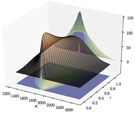
Figure 1. The derivative of Heston's call price w.r.t. the volatility σ₀.

FIGURE 2

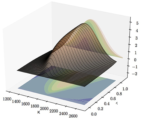
Figure 2. The derivative of Heston's call price w.r.t. the relaxation parameter κ.

FIGURE 3

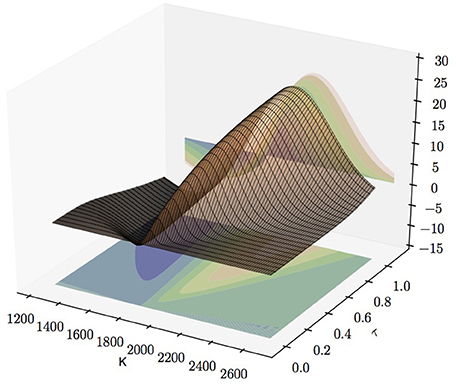
Figure 3. The derivative of Heston's call price w.r.t. the leverage parameter ρ.

FIGURE 4

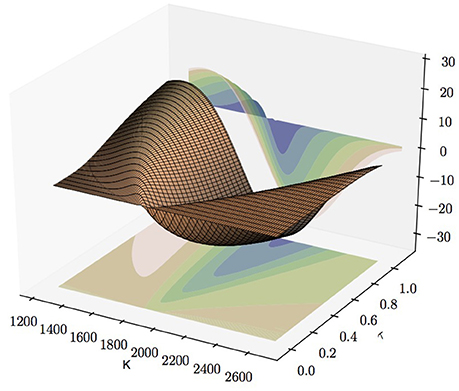
Figure 4. The derivative of Heston's call price w.r.t. the volatility of the variance process σ.

FIGURE 5

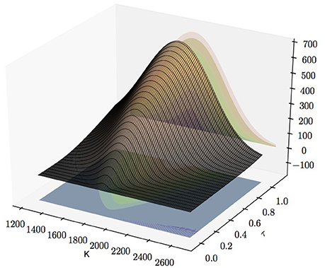
Figure 5. The derivative of Heston's call price w.r.t. the long-term mean of the volatility $\sqrt{\theta }$.

3.1.2. Vega-Drop

In general parameters are not estimated from a single option price but for various options over an entire time-period. An estimate over a time-period ${T}$ changes the picture in a twofold way. First, not only maturity and strikes vary but also volatility σ_t and the price of the underlying asset S_t. Second, since volatility σ_t needs to be estimated for every day $t\in {T}$ the parameter vector Θ is no longer $({\sigma }_0,\kappa ,\sqrt{\theta },\sigma ,\rho )$ but

$\begin{array}{rc}{({\sigma }_t)}_{t\in {T}}\oplus (\kappa ,\sqrt{\theta },\sigma ,\rho )& (3.1)\end{array}$

where ⊕ denotes concatenation. Consequently, the Fisher information matrix J(Θ) is an (m + 4) × (m + 4) matrix where $m=\left|{T}\right|$ is the number of days we consider. The first m diagonal elements of J(Θ)⁻¹ provide error variances on the estimates of volatilities ${({\sigma }_t)}_{{T}}$. According to lemma 2.1 these diagonal elements are lower bounded by

$\begin{array}{rc}\widehat{v}{\left(\frac{\partial }{\partial {\sigma }_t}{E}_t\right)}^{-2}\mathrm{\text{for}}t\in {T}& (3.2)\end{array}$

where E_t is an observed option price at time t. Hence, Vega, i.e., the first-order derivative of the option price w.r.t. volatility, plays a crucial role for error estimates for the majority of the parameters in Equation (3.1).

To investigate Vega in more detail, Figure 6 plots Vega of a European option traded on the S&P 500 over the same parameter set we have already applied for the explicit computation of the Greek-surfaces of the previous subsection: spot price S = 1,845.73, r = 0.167%, q = 1.894%, κ = 5.07, θ = 0.0457, σ = 0.48, ρ = −0.767, variance v = 0.0108, and maturity τ = 30 days, i.e., corresponding to a slice of the surface shown in Figure 1 at $\tau =\frac{30}{252}\approx 0.12$. As in the case of the classical Black Scholes Model, Vega is always positive, i.e., the value of an option increases with volatility, and Vega attains a maximum near the spot price of the underlying. Of greater importance is the dependency of Vega on the variance v if the strike is fixed.

FIGURE 6

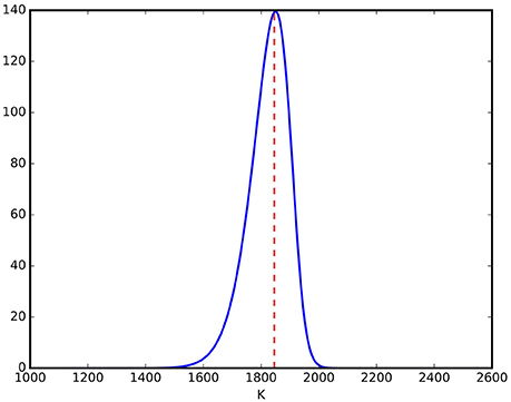
Figure 6. Vega for a European option priced by Heston's model over various strikes. It is strictly positive and has a global maximum near the spot price of the underlying asset (indicated by the red dashed line).

Figure 7 plots Vega in Heston's model for an at-the-money option over various variances for three different maturities: 23, 30, and 37 days; the range of maturities of the components of the VIX which is studied in the subsequent section. The curves for different maturities τ ∈ [23, 37] are located in the shaded region. One observes a fast drop of Vega for small variances v which is indicated by the dashed line corresponding to $\sqrt{v}=3\%$ corresponding to According to Equation (3.2) this fact sheds light on variance, and volatility estimates, respectively, from European options: if Vega decreases dramatically the error in estimating the volatility from options becomes large. In the subsequent section we show that this observed Vega-Drop is not only of theoretical but also practical interest if we investigate the quality of the VIX as a volatility proxy.

FIGURE 7

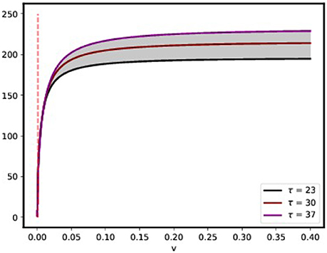
Figure 7. Vega for a European option price by Heston's model over various variances for a fixed strike K = 1,845.73 at the spot price of the underlying. Vega drops for small variances. The dashed line corresponds to $\sqrt{v}=3$%.

3.2. Fisher Information and the VIX

The S&P 500 is a major stock index which is calculated using the prices of approximately 500 component stocks of the biggest companies in the US. The S&P 500, like other indices, employs rules that govern the selection of the component securities and a formula to calculate index values. The VIX index measures 30-day expected volatility of the S&P 500 index and is comprised by options rather than stocks, with the price of each option reflecting the market's expectation of future volatility. Like conventional indices, the VIX calculation employs rules for selecting component options and a formula to calculate index values. Roughly, the selection filters near- and next-term put and call options with more than 23 days and less than 37 days to expiration and non-vanishing bid—see Chicago Board Options Exchange [22] for further details. With the aid of the OPTION METRICS database we are able to replicate the part of the portfolio¹ of options entering the calculation of the VIX from October 16th 2003 until August 31th 2015. Assuming that all prices of the VIX components are centered on the theoretical price Equation (2.3) in Heston's model disturbed by additive Gaussian Noise we address two questions to the data: first, how reliably can volatility be inferred from the VIX components; second, does the VIX really measure 30-day expected volatility if one considers the VIX index as a 30-day variance swap traded on the S&P 500? We tackle both questions in terms of Fisher information.

3.2.1. Inferring Volatility

We denote with ${{E}}_t={{C}}_t\cup {{P}}_t$ the set of all components of the VIX at day t where ${{C}}_t$ denotes the set of call options and ${{P}}_t$ the set of put options, respectively. We introduce the set ${T}=\left\{16/10/2003,17/10/2003,\dots ,31/08/2015\right\}$ of all trading days from October 16th 2003 until August 31th 2015. We assume that the price e_t of an option e in the set ${{E}}_t$ is normally distributed

$\begin{array}{l}p(e_t|ϵ,x_t,v_t,r_t,\kappa ,\theta ,\rho ,\sigma ,k_e,\tau )\\ =\frac{1}{\sqrt{2\pi \widehat{v}}}\exp \left(\frac{(e_t-E(ϵ,x_t,v_t,r_t,\kappa ,\theta ,\rho ,\sigma ,k_e,\tau ))}{2\widehat{v}}\right)\end{array}$

with a fixed variance $\widehat{v}$ and mean E(ϵ, x_t, v_t, r_t, κ_e, θ, ρ, σ, k, τ) provided by Equation (2.2) where x_t is the log-closing-price of the S&P 500 at day t, r_t the zero Coupon Bond yield at day t with maturity τ, and k_e the log-strike of the option. Beside the option prices, also the daily zero Coupon Bond yield r and the closing prices of the S&P 500 are provided by the OPTION METRICS database. Furthermore we adopt the estimate in Aït-Sahalia and Kimmel [21] for the parameters of the stochastic volatility process Equation (2.1).

$\begin{array}{rc}\kappa =5.07,\theta =0.0457,\sigma =0.48,\rho =-0.767& (3.3)\end{array}$

We fit the volatility with daily time-resolution on option data via a maximum likelihood estimate on the call option prices. That is, for every day $t\in {T}$, the variance v_t, and therefore volatility ${\sigma }_t=\sqrt{v_t}$, is determined as the maximum of the joint, negative log-likelihood function

$\begin{array}{l}-{\displaystyle \sum _{e\in {{E}}_t}}log(p(e_t|ϵ,x_t,v_t,r_t,\kappa ,\theta ,\rho ,\sigma ,k_c,\tau ))\end{array}$

which is equivalent to minimize the square-error

$\begin{array}{l}{\displaystyle \sum _{e\in {{E}}_t}}||e_t-E(ϵ,x_t,v_t,r_t,\kappa ,\theta ,\rho ,\sigma ,k_c,\tau )|{|}^2.\end{array}$

This procedure yields a time series ${(v_t)}_{t\in {T}}$ for the variance. Besides, the variance $\widehat{v}$ is obtained from maximizing the negative, joint log-likelihood function

$\begin{array}{l}{\displaystyle \sum _{t\in {T}}}{\displaystyle \sum _{e\in {{E}}_t}}log(p(e_t|ϵ,x_t,v_t,r_t,\kappa ,\theta ,\rho ,\sigma ,k_e,\tau ))\end{array}$

which yields the expression

$\begin{array}{l}\widehat{v}=\frac{1}{N}{\displaystyle \sum _{t\in {T}}}{\displaystyle \sum _{e\in {{E}}_t}}||e_t-E(ϵ,x,v_t,r,\kappa ,\theta ,\rho ,\sigma ,k_e,\tau )|{|}^2\end{array}$

where N is the cardinality of the union ${\bigcup }_{t\in {T}}{{E}}_t$. For our data set of options from October 16th 2003 until August 31st 2015 we obtain the value

$\begin{array}{l}\widehat{v}=0.2952.\end{array}$

corresponding to a standard deviation of about half a dollar.

We have assembled all necessary ingredients to tackle the following thought problem: how precisely can the volatlity ${({\sigma }_t)}_{t\in {T}}$, with ${\sigma }_t=\sqrt{v_t}$, and the parameters $\kappa ,\sqrt{\theta },\sigma$, and ρ be estimated from the components of the VIX? Since we are dealing with a lot of data, roughly several hundred option prices every day for estimating the daily volatility σ_t, and about three hundred thousand option prices are available for an estimation of the parameters $\kappa ,\sqrt{\theta },\sigma$ and ρ, we apply insights from asymptotic statistics [14] to quantifity the uncertainty left about the parameters

$\begin{array}{rc}\Theta ={({\sigma }_t)}_{t\in {T}}\oplus (\kappa ,\sqrt{\theta },\sigma ,\rho )& (3.4)\end{array}$

supposed they are fitted via a maximum likelihood estimate from the log-likelihood function

$\begin{array}{l}{\displaystyle \sum _{t\in {T}}}{\displaystyle \sum _{e\in {{E}}_t}}log(p(e_t|ϵ,x_t,v_t,r_t,\kappa ,\theta ,\rho ,\sigma ,k_e,\tau )).\end{array}$

Then, under fairly mild conditions, the maximum likelihood estimator is asymptotically normally distributed with mean Θ and covariance matrix J(Θ)⁻¹ where J(Θ) denotes the Fisher information matrix which adopts in the present context the block structure

$\begin{array}{rc}J(\Theta )=\frac{1}{\widehat{v}}\left(\begin{array}{cc}{\text{A}}_{11}& {\text{A}}_{12}\\ {\text{A}}_{21}& {\text{A}}_{22}\end{array}\right).& (3.5)\end{array}$

A₁₁ = (a_ij) is an m × m diagonal matrix, where m is the cardinality of ${T}$ s.t.

$\begin{array}{l}{a}_{ii}={\left({\partial }_{{\sigma }_{t_i}}{E}_i\right)}^2=4v_{t_i}{\left({\partial }_{v_{t_i}}{E}_i\right)}^2\end{array}$

where we write

$\begin{array}{rc}{E}_i={\displaystyle \sum _{e\in {{E}}_{t_i}}}E(ϵ,x_{t_i},v_{t_i},r_{t_i},\kappa ,\theta ,\rho ,\sigma ,k_e,\tau ).& (3.6)\end{array}$

A₁₂ is an m × 4 matrix,

$\begin{array}{l}{\text{A}}_{12}=\left(\begin{array}{cccc}{\partial }_{{\sigma }_{t_0}}{E}_0{\partial }_{\kappa }{E}_0& {\partial }_{{\sigma }_{t_0}}{E}_0{\partial }_{\sqrt{\theta }}{E}_0& {\partial }_{{\sigma }_{t_0}}{E}_0{\partial }_{\sigma }{E}_0& {\partial }_{{\sigma }_{t_0}}{E}_0{\partial }_{\rho }{E}_0\\ ⋮& ⋮& ⋮& ⋮\\ {\partial }_{{\sigma }_{t_m}}{E}_m{\partial }_{\kappa }{E}_m& {\partial }_{{\sigma }_{t_m}}{E}_m{\partial }_{\sqrt{\theta }}{E}_m& {\partial }_{{\sigma }_{t_m}}{E}_m{\partial }_{\sigma }{E}_m& {\partial }_{{\sigma }_{t_m}}{E}_m{\partial }_{\rho }{E}_m\end{array}\right),\end{array}$

and ${\text{A}}_{21}={\text{A}}_{12}^T$. Finally, A₂₂ is the 4 × 4 matrix

$\begin{array}{l}{\text{A}}_{22}={\displaystyle \sum _{i=1}^m}\nabla E_i\nabla E_i^T\end{array}$

where $\nabla E_i={({\partial }_{\kappa }{E}_i,{\partial }_{\theta }{E}_i,{\partial }_{\sigma }{E}_i,{\partial }_{\rho }{E}_i)}^T$ denotes the column gradient vector of E_i w.r.t. the parameters of the stochastic process Equation (2.1). If we assume that the previously fitted variance time-series ${(v_t)}_{t\in {T}}$ and the parameter set Equation (3.3) provide an estimator of Θ which is, like the maximum likelihood estimator, asymptotically normal with mean Θ and covariance matrix J(Θ)⁻¹, we can quantify the uncertainty left in our estimation in terms of the entries of the Fisher information matrix. Figure 8 presents the volatility time-series ${({\sigma }_t)}_{t\in {T}}$ obtained from the previously described fit on components entering the calculation of the VIX along with the uncertainty left.

FIGURE 8

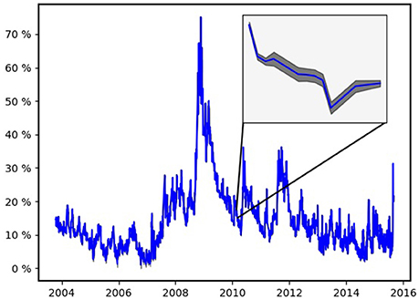
Figure 8. Volatility of the S&P 500. The close-up presents the volatility estimate along with its double standard deviation obtained from Fisher information matrix Equation (3.5).

Since the uncertainty left is negligible the shaded tube ${([{\sigma }_t-{\beta }_t,{\sigma }_t+{\beta }_t])}_{t\in {T}}$ (≈ 95% confidence interval) mantling the plot of the volatility time-series ${({\sigma }_t)}_{t\in {T}}$ is only visible in a close-up presented in Figure 8 as well. The close-up shows volatility from February 23rd 2010 until March 11th 2010 within a range from 13.5 till 18%. The boundaries ${({\beta }_t)}_{t\in {T}}$ of the confidence interval are obtained from the first m entries of the diagonal of the inverse $J{(\Theta )}^{-1}=({[J{(\Theta )}^{-1}]}_{ij})$ of the Fisher information matrix (Recall, m is the number of trading days we consider, i.e., the cardinality of the set ${T}$):

$\begin{array}{l}{\beta }_{t_i}=2\sqrt{{\left[J{(\Theta )}^{-1}\right]}_{ii}}\text{ for all }i=1,\dots ,m.\end{array}$

That is, in terms of asymptotic statistics, β_t is the double standard deviation of the asymptotically normal volatility estimate σ_t. On average the double standard deviation is

$\begin{array}{l}\overline{\beta }=\frac{1}{m}{\displaystyle \sum _{i=0}^m}{\beta }_{t_i}=0.0014.\end{array}$

The last four entries of the diagonal of $J{(\Theta )}^{-1}=({[J{(\Theta )}^{-1}]}_{ij})$ yield the variance of the estimates of the parameters $\kappa ,\sqrt{\theta },\sigma$ and ρ, respectively. Along with the parameter estimates of Aït-Sahalia and Kimmel [21] we obtain Table 1. Fitting the parameters $\kappa ,\sqrt{\theta },\sigma$, and ρ on options over a sufficiently long time-window yields fairly accurate estimates of them as well.

TABLE 1

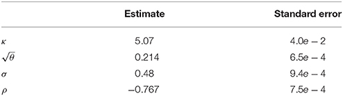
Table 1. The parameters of Heston's model along with their standard errors obtained from the Fisher information matrix if we assume they were estimated from the components of the VIX between October 16th 2003 until August 31st 2015.

Overall, estimates of hidden volatility and the parameters determining the stochastic process Equation (2.1) from option data appear reliable. Doubts are shed on these results if relative errors are considered instead of absolute ones. Figure 9 presents the relative uncertainty left, that is, the time-series ${({\beta }_t/{\sigma }_t)}_{t\in {T}}$. Apparently, the uncertainty becomes overwhelming, if the volatility drops. This is in accordance with the discussion in the previous section where we observed that Vega drops if volatility falls below a critical value. From the block structure Equation (3.5) of the Fisher information matrix and the proof of lemma 2.1 follows

$\begin{array}{l}{\left[J{(\Theta )}^{-1}\right]}_{ii}\ge \frac{\widehat{v}}{{({\partial }_{{\sigma }_{t_i}}{E}_i)}^2}\end{array}$

with E_i provided by Equation (3.6), and therefore

$\begin{array}{l}{\beta }_{t_i}\ge \frac{2\sqrt{\widehat{v}}}{{\partial }_{{\sigma }_{t_i}}{E}_i}\end{array}$

for all i = 1, …, m. Hence, there is a lower bound of the error of the volatility σ_t proportional to the inverse of a sum of Vegas. If this sum shrinks the error becomes large.

FIGURE 9

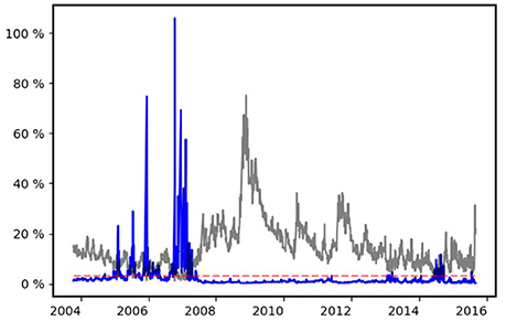
Figure 9. The relative error of the volatility estimate (blue line) and volatility itself (transparent black line). If volatility drops below 3% (dashed, transparent red line), option data yield little information about volatility.

3.2.2. The VIX as Variance Swap

The VIX is quoted in percentage points and translates, roughly, to the expected movement (with the assumption of a 68% likelihood, i.e., one standard deviation) in the S&P 500 index over the next 30-day period, which is then annualized. According to Carr and Wu [23] the VIX can also be considered as 30 day variance swap on the S&P 500. Recall Equation (2.1) that the variance of the Heston model is driven by the CIR process

$\begin{array}{l}d{v}_t=\kappa (\theta -v_t)dt+\sigma \sqrt{v_t}d{W}_t\end{array}$

and consequently, that the expected value of v_t conditional on v_s (s < t) is

$\begin{array}{l}𝔼\left[v_t|v_s\right]=v_s{e}^{-\kappa (t-s)}+\theta \left(1-e^{-\kappa (t-s)}\right)=(v_s-\theta )e^{-\kappa (t-s)}+\theta .\end{array}$

In the sequel, we make use of 𝔼[v_t|v_s] but with s = 0. It is useful to denote this quantity as ${\widehat{v}}_t$

$\begin{array}{l}{\widehat{v}}_t=𝔼\left[v_t|v_0\right]=(v_0-\theta )e^{-\kappa t}+\theta .\end{array}$

It is also useful to define the total (integrated) variance ŵ_t as

$\begin{array}{l}{ŵ}_t={\displaystyle {\int }_0^t}{v}_{s}ds=(v_0-\theta )\frac{1-e^{-\kappa t}}{\kappa }+\theta t.\end{array}$

As explained by Gatheral [24], a variance swap requires an estimate of the future variance over the (0, T) time period. This can be obtained as the conditional expectation of the integrated variance. A fair estimate of the total variance is therefore

$\begin{array}{l}𝔼\left[{\displaystyle {\int }_0^T}{v}_{t}dt|v_0\right]={\displaystyle {\int }_0^T}𝔼\left[v_t|v_0\right]dt\\ ={\displaystyle {\int }_0^T}(v_0-\theta )e^{-\kappa t}+\theta dt\\ =(v_0-\theta )\frac{1-e^{-\kappa T}}{\kappa }+\theta T\end{array}$

which is simply ŵ_T. Since this represents the total variance over (0, T), it must be scaled by T in order to represent a fair estimate of annual variance (assuming that T is expressed in years). Hence, the strike variance $K_{\mathrm{\text{var}}}^2$ for a variance swap is obtained by dividing this last expression by T

$\begin{array}{l}{K}_{\mathrm{\text{var}}}^2=(v_0-\theta )\frac{1-e^{-\kappa T}}{\kappa T}+\theta .\end{array}$

Returning to Carr's and Wu's [23] interpretation of the VIX the VIX-time series ${({\mathrm{\text{VIX}}}_t)}_{t\in {T}}$ is the time-series

$\begin{array}{l}{K}_{\mathrm{\text{var}},t}=\sqrt{(v_t-\theta )\frac{1-e^{-\kappa T}}{\kappa T}+\theta }\text{ for }t\in {T}\end{array}$

where ${(v_t)}_{t\in {T}}$ denotes the variance of the S&P 500 at day t and T = 30/365. Thus, Fisher information provides an uncertainty estimate on the VIX, considered as 30 days variance swap, estimated from its components, i.e., near- and next-term put and call options with more than 23 days and less than 37 days to expiration and non-vanishing bid. We only have to transform the Fisher information matrix already computed in the previous subsection according to the rules Equation (2.10). In terms of Equation (2.10) in section 2.1 we have

$\begin{array}{l}\Lambda ={(K_{\mathrm{\text{var}},t})}_{t\in {T}}\oplus (\kappa ,\sqrt{\theta },\sigma ,\rho )\\ \Theta ={({\sigma }_t)}_{t\in {T}}\oplus (\kappa ,\sqrt{\theta },\sigma ,\rho )\end{array}$

and

$\begin{array}{l}J(\Lambda )=D^{T}J(\Theta )D.\end{array}$

Hence, the transformation matrix D in Equation (2.10) adopts the block form

$\begin{array}{l}D=\left(\begin{array}{cc}{\text{A}}_{11}& {\text{A}}_{12}\\ {\text{A}}_{21}& {\text{A}}_{22}\end{array}\right).\end{array}$

A₁₁ is an m × m diagonal matrix with entries

$\begin{array}{l}{a}_{ii}=\frac{\partial {\sigma }_{t_i}}{\partial K_{\mathrm{\text{var}},t_i}}=\frac{\partial {\sigma }_{t_i}}{\partial v_{t_i}}\frac{\partial v_{t_i}}{\partial K_{\mathrm{\text{var}},t_i}}\\ =\frac{1}{2{\sigma }_{t_i}}\frac{\partial }{\partial K_{\mathrm{\text{var}},t_i}}\left(\frac{(K_{\mathrm{\text{var}},t_i}^2-\theta )\kappa T}{1-e^{-\kappa T}}+\theta \right)=\frac{1}{{\sigma }_{t_i}}\frac{K_{\mathrm{\text{var}},t_i}\kappa T}{1-e^{-\kappa T}}\end{array}$

for i = 1, …, m where m is the number of trading days $t_i\in {T}$ from October 16th 2003 until August 31st 2015. A₁₂ is an m × 4-matrix with entries

$\begin{array}{l}\left(\begin{array}{cccc}\frac{\partial {\sigma }_{t_0}}{\partial \kappa }& \frac{\partial {\sigma }_{t_0}}{\partial \sqrt{\theta }}& 0& 0\\ ⋮& ⋮& ⋮& ⋮\\ \frac{\partial {\sigma }_{t_m}}{\partial \kappa }& \frac{\partial {\sigma }_{t_m}}{\partial \sqrt{\theta }}& 0& 0\end{array}\right)\end{array}$

where

$\begin{array}{l}\frac{\partial {\sigma }_{t_i}}{\partial \kappa }=\frac{\partial {\sigma }_{t_i}}{\partial v_{t_i}}\frac{\partial v_{t_i}}{\partial \kappa }=\frac{(K_{\mathrm{\text{var}},t_i}^2-\theta )T}{2{\sigma }_{t_i}}\frac{\partial }{\partial \kappa }\left(\frac{\kappa }{1-e^{-\kappa T}}\right)\\ =\frac{(K_{\mathrm{\text{var}},t_i}^2-\theta )T}{2{\sigma }_{t_i}}\frac{1-(1+\kappa T)e^{-\kappa T}}{{(1-e^{-\kappa T})}^2}\\ \frac{\partial {\sigma }_{t_i}}{\partial \sqrt{\theta }}=\frac{\partial {\sigma }_{t_i}}{\partial v_{t_i}}\frac{\partial \theta }{\partial \sqrt{\theta }}\frac{\partial v_{t_i}}{\partial \theta }=\frac{\sqrt{\theta }}{{\sigma }_{t_i}}\left(1-\frac{\kappa T}{1-e^{-\kappa T}}\right).\end{array}$

Finally, ${\text{A}}_{21}={\text{A}}_{12}^T$ and A₂₂ is the 4 × 4 identity matrix. Similar to Figure 8 we plot Figure 10 the time-series ${(K_{\mathrm{\text{var}},t})}_{t\in {T}}$ along with its 95% confidence region [K_{var, t} − β_t, K_{var, t} + β_t] where

$\begin{array}{l}{\beta }_{t_i}=2\sqrt{{\left[J{(\Lambda )}^{-1}\right]}_{ii}}\text{ for }i=1,\dots ,m.\end{array}$

FIGURE 10

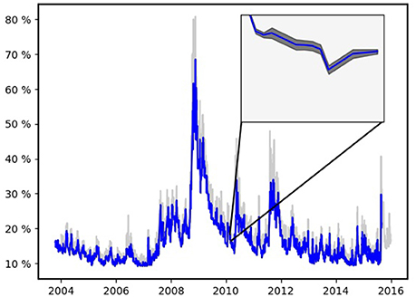
Figure 10. The time series ${(K_{\mathrm{\text{var}},t})}_{t\in {T}}$. The close-up shows the graph along with its 95% confidence region. The gray transparent line shows the historical VIX.

Furthermore, the historical VIX is plotted. The value K_{var, t} is systematically smaller than the realized VIX. This is most likely due to the fact that the formulae for the realized VIX computes implied volatilities using the Black-Scholes model whereas our estimate is derived from the Heston model which can replicate the volatility smile, i.e., does not systematically overestimate the volatility of out of the money options.

As for the volatility the error is negligible and on average we have

$\begin{array}{l}\bar{\beta }=\frac{1}{m}{\displaystyle \sum _{i=0}^m}{\beta }_{t_i}=8.9e-04.\end{array}$

Compared to the volatility estimates from options there is big difference if we consider the relative error, that is, the time-series β_t/K_{var, t} for $t\in {T}$ in Figure 11. The relative error never exceeds 3%.

FIGURE 11

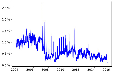
Figure 11. The time series ${({\beta }_t/K_{\mathrm{\text{var}},t})}_{t\in {T}}$, i.e., the relative error of the VIX estimate K_{var, t}.

4. Discussion

Here, we have addressed the question of how reliably volatility can be estimated from option price data. To this end, we computed the Fisher information matrix of Heston's stochastic volatility model. Thanks to the analytic tractability of Heston's model, the Fisher information can be expressed in Fourier integrals giving the Heston Greeks.

Our investigations lead to the following insights: First, volatility estimation from market data as exemplified on S&P 500 index options is reliable most of the time, with occasional large relative errors for very low volatilities. Low volatilities are hard to estimate as Vega almost vanishes in this case, making it impossible to extract information from option prices. Second, options at the money are most informative about volatility while almost no information can be obtained from options that are far out of the money. We might speculate that this could lead to overconfident estimates of portfolio risk especially in times of calm financial markets. Nevertheless, the VIX index itself, reflecting the average volatility over the next month, proves to be an accurate accessment of volatility.

Overall, this work complements our previous findings [12] regarding the low information content of stock returns. There we computed the mutual information between stock returns and their hidden volatility for a wide class of stochastic volatility models including Heston's. Our results showed that in general at least secondly quoted return data is necessary to infer volatility with a precision comparable to the VIX quoted at 0.01%. We speculated that option price data could lead to much more reliable volatility estimates as confirmed by the analysis presented here.

Author Contributions

The research was initiated by NB. Calculations and numerical studies were carried out by OP. Both authors have written and agreed on the final manuscript.

Funding

NB and OP thank Dr. h.c. Maucher for funding their positions.

Conflict of Interest Statement

The authors declare that the research was conducted in the absence of any commercial or financial relationships that could be constr ued as a potential conflict of interest.

Footnotes

1. ^The new VIX is computed based on S&P 500 options which strike dates are renewed in monthly intervals. In addition, weekly options, traded under a different ticker, are used to cover the remaining weeks. These later options are not available in our data base.

References

1. Brenner M, Galai D. New financial instruments for hedging changes in volatility. Finan Anal J. (1989) 45:61–5. doi: 10.2469/faj.v45.n4.61

CrossRef Full Text | Google Scholar

2. Brenner M, Galai D. Hedging volatility in foreign currencies. J Derivat. (1993) 1:53–9.

3. Bouchaud JP, Potters M. Theory of financial risk and derivative pricing. New York, NY: Cambridge University Press (2003). p. 379. doi: 10.1017/CBO9780511753893

CrossRef Full Text | Google Scholar

4. Perello J, Sircar R, Masoliver J. Option pricing under stochastic volatility: the exponential Ornstein-Uhlenbeck model. arXiv:08042589. (2008). p. 26. Available online at: http://arxiv.org/abs/0804.2589

Google Scholar

5. Muzy JF, Delour J, Bacry E. Modelling fluctuations of financial time series: from cascade process to stochastic volatility model. Eur Phys J B. (2000) 17:537–48. doi: 10.1007/s100510070131

CrossRef Full Text | Google Scholar

6. Lo AW. Long term memory in stock market prices. Econometrica (1991) 59:1279–313. doi: 10.2307/2938368

CrossRef Full Text | Google Scholar

7. Ding Z, Granger CWJ, Engle RF. A long memory property of stock market returns and a new model. J Empir Finance (1993) 1:83–106. doi: 10.1016/0927-5398(93)90006-D

CrossRef Full Text | Google Scholar

8. LeBaron B. Stochastic Voltility as a Simple Generator of apparent financial power laws and long memory. Quant Finance (2001) 6:627–31. doi: 10.1088/1469-7688/1/6/304

CrossRef Full Text

9. Bouchaud JP, Matacz a, Potters M. Leverage effect in financial markets: the retarded volatility model. Phys Rev Lett. (2001) 87:228701. doi: 10.1103/PhysRevLett.87.228701

PubMed Abstract | CrossRef Full Text | Google Scholar

10. Black F, Scholes M. The pricing of options and corporate liabilities. J Polit Econ. (1973) 81:637.

Google Scholar

11. Bollerslev T, Litvinova J, Tauchen G. Leverage and volatility feedback effects in high-frequency data. J Finan Econometr. (2006) 4:353–84. doi: 10.1093/jjfinec/nbj014

CrossRef Full Text | Google Scholar

12. Pfante O, Bertschinger N. Volatility inference and return dependencies in stochastic volatility models. arXiv:161000312 [q-finMF]. (2016).

Google Scholar

13. Heston SL. A closed-form solution for options with stochastic volatility with applications to bond and currency options. Rev Finan Stud. (1993) 6:327–43.

Google Scholar

14. Ibragimov IA, Has'minskii RZ. Statistical Estimation – Asymptotic Theory. New York, NY: Springer (1981).

Google Scholar

15. Rouah FD. The Heston Model and Its Extensions in Matlab and C#. Hoboken, NJ: Wiley (2013).

Google Scholar

16. Carr P, Madan D. Option valuation using the fast Fourier transform. J Comput Finance (1999) 2:61–73.

Google Scholar

17. Albrecher H, Mayer P, Schoutens W, Tistaert J. The little heston trap. Wilmott Mag. (2007) 83–92.

18. Chourdakis K. Option pricing using the fractional FFT. J Comput Finance (2005) 8:1–18. doi: 10.21314/JCF.2005.137

CrossRef Full Text | Google Scholar

19. Cover TM, Thomas JA. Elements of Information Theory, 2nd edn. Hoboken, NJ: Wiley-Interscience (2006).

20. Petersen KB, Pedersen MS. The Matrix Cookbook. (2012). Available online at: http://matrixcookbook.com

21. Aït-Sahalia Y, Kimmel R. Maximum likelihood estimation of stochastic volatility models. J Finan Econ. (2007) 83:413–52. doi: 10.1016/j.jfineco.2005.10.006

CrossRef Full Text | Google Scholar

22. Chicago Board Options Exchange. The CBOE Volatility Index - VIX. White Paper. (2004). Available online at: http://matrixcookbook.com

23. Carr P, Wu L. A Tale of Two Indices. NYU Working Paper No SC-CFE-04-01 (2014).

24. Gatheral J. The Volatility Surface: A Practitioner's Guide. Hoboken, NJ: John Wiley & Sons (2011).

Google Scholar