Exact Heat Kernel on a Hypersphere and Its Applications in Kernel SVM

1. Introduction

As the techniques for analyzing large data sets continue to grow, diverse quantitative sciences—including computational biology, observation astronomy, and high energy physics—are becoming increasingly data driven. Moreover, modern business decision making critically depends on quantitative analyses such as community detection and consumer behavior prediction. Consequently, statistical learning has become an indispensable tool for modern data analysis. Data acquired from various experiments are usually organized into an n × m matrix, where the number n of features typically far exceeds the number m of samples. In this view, the m samples, corresponding to the columns of the data matrix, are naturally interpreted as points in a high-dimensional feature space ℝⁿ. Traditional statistical modeling approaches often lose their power when the feature dimension is high. To ameliorate this problem, Lafferty and Lebanon proposed a multinomial interpretation of non-negative feature vectors and an accompanying transformation of the multinomial simplex to a hypersphere, demonstrating that using the heat kernel on this hypersphere may improve the performance of kernel support vector machine (SVM) [2–8]. Despite the interest that this idea has attracted, only approximate heat kernel is known to date. We here present an exact form of the heat kernel on a hypersphere of arbitrary dimension and study its performance in kernel SVM classifications of text mining, genomic, and stock price data sets.

To date, sparse data clouds have been extensively analyzed in the flat Euclidean space endowed with the L²-norm using traditional statistical learning algorithms, including KMeans, hierarchical clustering, SVM, and neural network [2–8]; however, the flat geometry of the Euclidean space often poses severe challenges in clustering and classification problems when the data clouds take non-trivial geometric shapes or class labels are spatially mixed. Manifold learning and kernel-based embedding methods attempt to address these challenges by estimating the intrinsic geometry of a putative submanifold from which the data points were sampled and by embedding the data into an abstract Hilbert space using a nonlinear map implicitly induced by the chosen kernel, respectively [9–11]. The geometry of these curved spaces may then provide novel information about the structure and organization of original data points.

Heat equation on the data submanifold or transformed feature space offers an especially attractive idea of measuring similarity between data points by using the physical model of diffusion of relatedness (“heat”) on curved space, where the diffusion process is driven by the intrinsic geometry of the underlying space. Even though such diffusion process has been successfully approximated as a discrete-time, discrete-space random walk on complex networks, its continuous formulation is rarely analytically solvable and usually requires complicated asymptotic expansion techniques from differential geometry [12]. An analytic solution, if available, would thus provide a valuable opportunity for comparing its performance with approximate asymptotic solutions and rigorously testing the power of heat diffusion for geometric data analysis.

Given that a Riemannian manifold of dimension d is locally homeomorphic to ℝ^d, and that the heat kernel is a solution to the heat equation with a point source initial condition, one may assume in the short diffusion time limit (t ↓ 0) that most of the heat is localized within the vicinity of the initial point and that the heat kernel on a Riemannian manifold locally resembles the Euclidean heat kernel. This idea forms the motivation behind the parametrix expansion, where the heat kernel in curved space is approximated as a product of the Euclidean heat kernel in normal coordinates and an asymptotic series involving the diffusion time and normal coordinates. In particular, for a unit hypersphere, the parametrix expansion in the limit t ↓ 0 involves a modified Euclidean heat kernel with the Euclidean distance ||x|| replaced by the geodesic arc length θ. Computing this parametrix expansion is, however, technically challenging; even when the computation is tractable, applying the approximation directly to high-dimensional clustering and classification problems may have limitations. For example, in order to be able to group samples robustly, one needs the diffusion time t to be not too small; otherwise, the sample relatedness may be highly localized and decay too fast away from each sample. Moreover, the leading order term in the asymptotic series is an increasing function of θ and diverges as θ approaches π, yielding an incorrect conclusion that two antipodal points are highly similar. For these reasons, the machine learning community has been using only the Euclidean diffusion term without the asymptotic series correction; how this resulting kernel, called the parametrix kernel [1], compares with the exact heat kernel on a hypersphere remains an outstanding question, which is addressed in this paper.

Analytically solving the diffusion equation on a Riemannian manifold is challenging [12–14]. Unlike the discrete analogs—such as spectral clustering [15] and diffusion map [16], where eigenvectors of a finite dimensional matrix can be easily obtained—the eigenfunctions of the Laplace operator on a Riemannian manifold are usually intractable. Fortunately, the high degree of symmetry of a hypersphere allows the explicit construction of eigenfunctions, called hyperspherical harmonics, via the projection of homogeneous polynomials [17, 18]. The exact heat kernel is then obtained as a convergent power series in these eigenfunctions. In this paper, we compare the analytic behavior of this exact heat kernel with that of the parametrix kernel and analyze their performance in classification.

2. Results

The heat kernel is the fundamental solution to the heat equation (∂_t − Δ_x)u(x, t) = 0 with an initial point source [19], where Δ_x is the Laplace operator; the amount of heat emanating from the source that has diffused to a neighborhood during time t > 0 is used to measure the similarity between the source and proximal points. The heat conduction depends on the geometry of feature space, and the main idea behind the application of hyperspherical geometry to data analysis relies on the following map from a non-negative feature space to a unit hypersphere:

Definition 1. A hyperspherical map $\phi :{ℝ}_{\ge 0}^n\backslash \{0\}\to S^{n-1}$ maps a vector x, with x_i ≥ 0 and $\sum _{i=1}^n{x}_i>0$, to a unit vector $\widehat{x}\in S^{n-1}$ where ${(\widehat{x})}_i\equiv \sqrt{x_i/\sum _{j=1}^n{x}_j}$.

We will henceforth denote the image of a feature vector x under the hyperspherical map as $\widehat{x}$. The notion of neighborhood requires a well-defined measurement of distance on the hypersphere, which is naturally the great arc length—the geodesic on a hypersphere. Both parametrix approximation and exact solution employ the great arc length, which is related to the following definition of cosine similarity:

Definition 2. The generic cosine similarity between two feature vectors x, y ∈ ℝⁿ\{0} is

$\cos \theta \equiv \frac{x·y}{\Vert x\Vert \Vert y\Vert },$

where ||·|| is the Euclidean L²-norm, and θ ∈ [0, π] is the great arc length on S^{n − 1}. For unit vectors $\widehat{x}=\phi (\text{x})$ and ŷ = φ(y) obtained from non-negative feature vectors $\text{x},\text{y}\in {ℝ}_{\ge 0}^n\backslash \{0\}$ via the hyperspherical map, the cosine similarity reduces to the dot product $cos\theta =\widehat{x}·\widehat{y}$; the non-negativity of x and y guarantees that θ ∈ [0, π/2] in this case.

2.1. Parametrix Expansion

The parametrix kernel K^prx previously used in the literature is just a Gaussian RBF function with $\theta =arccos\widehat{x}·\widehat{y}$ as the radial distance [1]:

Definition 3. The parametrix kernel is a non-negative function

$K^{\text{prx}}(\widehat{x},\widehat{y};t)={\text{e}}^{-\frac{{\arccos }^2\widehat{x}·\widehat{y}}{4t}}={\text{e}}^{-\frac{{\theta }^2}{4t}},$

defined for t > 0 and attaining global maximum 1 at θ = 0.

Note that this kernel is assumed to be restricted to the positive orthant. The normalization factor ${(4\pi t)}^{-\frac{n-1}{2}}$ is numerically unstable as t ↓ 0 and complicates hyperparameter tuning; as a global scaling factor of the kernel can be absorbed into the misclassification C-parameter in SVM, this overall normalization term is ignored in this paper. Importantly, the parametrix kernel K^prx is merely the Gaussian multiplicative factor without any asymptotic expansion terms in the full parametrix expansion G^prx of the heat kernel on a hypersphere [1, 12], as described below. The leading order term in the full parametrix expansion was derived in Berger et al. [12] and quoted in Lafferty and Lebanon [1]. For the sake of completeness, we include the details here and also extend the calculation to higher order terms.

The Laplace operator on manifold ${M}$ equiped with a Riemannian metric g_μν acts on a function f that depends only on the geodesic distance r from a fixed point as

$\begin{array}{ll}\Delta f(r)=f^{″}(r)+{\left(\log \sqrt{g}\right)}^{\prime }{f}^{\prime }(r),& (1)\end{array}$

where g ≡ det(g_μν) and ′ denotes the radial derivative. Due to the nonvanishing metric derivative in Equation (1), the canonical diffusion function

$\begin{array}{ll}G(r,t)={\left(\frac{1}{4\pi t}\right)}^{\frac{d}{2}}\exp \left(-\frac{r^2}{4t}\right)& (2)\end{array}$

does not satisfy the heat equation; that is, (Δ − ∂_t)G(r, t) ≠ 0 (Supplementary Material, section 2). For sufficiently small time t and geodesic distance r, the parametrix expansion of the heat kernel on a full hypersphere proposes an approximate solution

$K_p(r,t)=G(r,t)\left(u_0(r)+u_1(r)t+u_2(r)t^2+\cdots +u_p(r)t^p\right),$

where the functions u_i should be found such that K_p satisfies the heat equation to order t^p−d/2, which is small for t ≪ 1 and p > d/2; more precisely, we seek u_i such that

$\begin{array}{ll}(\Delta -{\partial }_t)K_p=G{t}^p\Delta u_p.& (3)\end{array}$

Taking the time derivative of K_p yields

$\begin{array}{l}{\partial }_t{K}_p=G·[\left(-\frac{d}{2t}+\frac{r^2}{4t^2}\right)\left(u_0+u_{1}t+u_2{t}^2+\cdots +u_p{t}^p\right)\\ +\left(u_1+2u_{2}t+\cdots +p{u}_p{t}^{p-1}\right)],\end{array}$

while the Laplacian of K_p is

$\begin{array}{l}\Delta K_p=\left(u_0+u_{1}t+\cdots +u_p{t}^p\right)\Delta G\\ +G\Delta \left(u_0+u_{1}t+\cdots +u_p{t}^p\right)\\ +2G^{\prime }{\left(u_0+u_{1}t+\cdots +u_p{t}^p\right)}^{\prime }.\end{array}$

One can easily compute

$\Delta G=\left[\left(-\frac{1}{2t}+\frac{r^2}{4t^2}\right)-\frac{r}{2t}{(\log \sqrt{g})}^{\prime }\right]G$

and

$G^{\prime }{\left(u_0+u_{1}t+\cdots \right)}^{\prime }=-\frac{r}{2t}\left(u_0^{\prime }+u_1^{\prime }t+\cdots \right)G.$

The left-hand side of Equation (3) is thus equal to G multiplied by

$\begin{array}{l}\left(u_0+\cdots +u_p{t}^p\right)\left[-\frac{r}{2t}(\log \sqrt{g}{)}^{\prime }+\frac{d-1}{2t}\right]+\Delta \left(u_0+\cdots +u_p{t}^p\right)+\\ -\frac{r}{t}\left(u_0^{\prime }+\cdots +u_p^{\prime }{t}^p\right)-\left(u_1+2u_{2}t+\cdots +p{u}_p{t}^{p-1}\right),\end{array}$

and we need to solve for u_i such that all the coefficients of t^q in this expression, for q < p, vanish.

For q = −1, we need to solve

$u_0\frac{r}{2}\left[-(\log \sqrt{g}{)}^{\prime }+\frac{d-1}{r}\right]=r{u}_0^{\prime },$

or equivalently,

${\left(\log u_0\right)}^{\prime }=-\frac{1}{2}(\log \sqrt{g}{)}^{\prime }+\frac{d-1}{2r}.$

Integrating with respect to r yields

$\log u_0=-\frac{1}{2}\left[\log \sqrt{g}-(d-1)\log r\right]+\text{const}.,$

where we implicitly take only the radial part of $log\sqrt{g}$. Thus, we get

$u_0=\text{const}.\times {\left(\frac{\sqrt{g}}{r^{d-1}}\right)}^{-\frac{1}{2}}\propto {\left(\frac{\sin r}{r}\right)}^{-\frac{d-1}{2}}$

as the zeroth-order term in the parametrix expansion. Using this expression of u₀, the remaining terms become

$\begin{array}{l}r\left[\left(u_1+u_{2}t+\cdots \right)(\log u_0{)}^{\prime }-\left(u_1^{\prime }+u_2^{\prime }t+\cdots \right)\right]+\\ +\left(\Delta u_0+t\Delta u_1+\cdots \right)-\left(u_1+2u_{2}t+\cdots \right),\end{array}$

and we obtain the recursion relation

$u_{k+1}(\log u_0{)}^{\prime }-u_{k+1}^{\prime }=-\frac{\Delta u_k-(k+1)u_{k+1}}{r}.$

Algebraic manipulations show that

$(\log r^{k+1}-\log u_0+\log u_{k+1}{)}^{\prime }{u}_{k+1}=r^{-1}\Delta u_k,$

from which we get

${\left(\frac{u_{k+1}{r}^{k+1}}{u_0}\right)}^{\prime }=r^{(k+1)-1}{u}_0^{-1}\Delta u_k.$

Integrating this equation and rearranging terms, we finally get

$\begin{array}{ll}{u}_{k+1}=r^{-(k+1)}{u}_0{\displaystyle {\int }_0^{r}d}\tilde{r}{\tilde{r}}^k{u}_0^{-1}\Delta u_k.& (4)\end{array}$

Setting k = 0 in this recursion equation, we find the second correction term to be

$\begin{array}{l}{u}_1=\frac{u_0}{r}{\displaystyle {\int }_0^{r}d}\tilde{r}{u}_0^{-1}\Delta u_0\\ =\frac{u_0}{r}{\displaystyle {\int }_0^{r}d}\tilde{r}{u}_0^{-1}\left(u_0^{″}+u_0^{\prime }(\log \sqrt{g}{)}^{\prime }\right).\end{array}$

From our previously obtained solution for u₀, we find

$u_0^{\prime }=\frac{1}{2}\left(\frac{d-1}{r}-\frac{g^{\prime }}{2g}\right)u_0,$

and

$u_0^{″}=\frac{1}{4}\left[\frac{(d-1)(d-3)}{r^2}-\frac{g^{\prime }(d-1)}{gr}-\frac{g^{″}}{g}+\frac{5}{4}{\left(\frac{g^{\prime }}{g}\right)}^2\right]u_0.$

Substituting these expressions into the recursion relation for u₁ yields

$u_1=\frac{u_0}{4r}{\displaystyle {\int }_0^{r}d}r\left[\frac{(d-1)(d-3)}{r^2}-\frac{g^{″}}{g}+\frac{3}{4}{\left(\frac{g^{\prime }}{g}\right)}^2\right].$

For the hypersphere S^d, where d ≡ n − 1 and g = const. × sin^{2(d − 1)}r, we have

$\frac{g^{\prime }}{g}=\frac{2(d-1)}{\tan r}$

and

$\frac{g^{″}}{g}=2(d-1)\left(\frac{2d-3}{{\tan }^{2}r}-1\right).$

Thus,

$\begin{array}{l}{u}_1=\frac{u_0}{4r}{\displaystyle {\int }_0^{r}d}\tilde{r}\left[\frac{(d-1)(d-3)}{{\tilde{r}}^2}-(d-1)\left(\frac{d-3}{{\tan }^2\tilde{r}}-2\right)\right]\\ =\frac{u_0(d-1)}{4r^2}\left[3-d+(d-1)r^2+(d-3)r\cot r\right].& (5)\end{array}$

Notice that u₁(r) = 0 when d = 1 and u₁(r) = u₀(r) when d = 3. For d = 2, u₁/u₀ is an increasing function in r and diverges to ∞ at r = π. By contrast, for d > 3, u₁/u₀ is a decreasing function in r and diverges to −∞ at r = π; u₁/u₀ is relatively constant for r < π and starts to decrease rapidly only near π. Therefore, the first order correction is not able to remove the unphysical behavior near r = 0 in high dimensions where, according to the first order parametrix kernel, the surrounding area is hotter than the heat source.

Next, we apply Equation (4) again to obtain u₂ as

$\begin{array}{l}{u}_2=\frac{u_0}{r^2}{\displaystyle {\int }_0^{r}d}\tilde{r}\tilde{r}{u}_0^{-1}\Delta u_1\\ =\frac{u_0}{r^2}{\displaystyle {\int }_0^{r}d}\tilde{r}\tilde{r}{u}_0^{-1}\left(u_0^{″}+u_1^{\prime }(\log \sqrt{g}{)}^{\prime }\right).\end{array}$

After some cumbersome algebraic manipulations, we find

$\begin{array}{l}\frac{u_2}{u_0}=\frac{d-1}{32}[{(d-3)}^3+\frac{(d-3)(d-5)(d-7)}{r^4}-\frac{{(d-3)}^2(d-5)}{r^3\tan r}\\ +\frac{2{(d-1)}^2(d-3)}{r\tan r}+\frac{(d+1)(d-3)(d-5)}{r^2\sin r}].& (6)\end{array}$

Again, d = 1 and d = 3 are special dimensions, where u₂(r) = 0 for d = 1, and u₂(r) = u₀/2 for d = 3; for other dimensions, u₂(r) is singular at both r = 0 and π. Note that on S¹, the metric in geodesic polar coordinate is g₁₁ = 1, so all parametrix expansion coefficients u_k(r) must vanish identically, as we have explicitly shown above.

Thus, the full G^prx defined on a hypersphere, where the geodesic distance r is just the arc length θ, suffers from numerous problems. The zeroth order correction term $u_0={(sin\theta /\theta )}^{-\frac{n-2}{2}}$ diverges at θ = π; this behavior is not a major problem if θ is restricted to the range $\left[0,\frac{\pi }{2}\right]$. Moreover, G^prx is also unphysical as θ ↓ 0 when (n − 2)t > 3; this condition on dimension and time is obtained by expanding ${\text{e}}^{-{\theta }^2/4t}=1-\frac{{\theta }^2}{4t}+{O}({\theta }^4)$ and ${(sin\theta /\theta )}^{-\frac{n-2}{2}}=1+\frac{{\theta }^2}{12}(n-2)+{O}({\theta }^3)$, and noting that the leading order θ² term in the product of the two factors is a non-decreasing function of distance θ when $\frac{n-2}{12}\ge \frac{1}{4t}$, corresponding to the unphysical situation of nearby points being hotter than the heat source itself. As the feature dimension n is typically very large, the restriction (n − 2)t < 3 implies that we need to take the diffusion time to be very small, thus making the similarity measure captured by G^prx decay too fast away from each data point for use in clustering applications. In this work, we further computed the first and second order correction terms, denoted u₁ and u₂ in Equations (5), (6), respectively. In high dimensions, the divergence of u₁/u₀ and u₂/u₀ at θ = π is not a major problem, as we expect the expansion to be valid only in the vicinity θ ↓ 0; however, the divergence of u₂/u₀ at θ = 0 (to −∞ in high dimensions) is pathological, and thus, we truncate our approximation to ${O}(t^2)$. Since u₁(θ) is not able to correct the unphysical behavior of the parametrix kernel near θ = 0 in high dimensions, we conclude that the parametrix approximation fails in high dimensions. Hence, the only remaining part of G^prx still applicable to SVM classification is the Gaussian factor, which is clearly not a heat kernel on the hypersphere. The failure of this perturbative expansion using the Euclidean heat kernel as a starting point suggests that diffusion in ℝ^d and S^d are fundamentally different and that the exact hyperspherical heat kernel derived from a non-perturbative approach will likely yield better insights into the diffusion process.

2.2. Exact Hyperspherical Heat Kernel

By definition, the exact heat kernel $G^{\text{ext}}(\widehat{x},\widehat{y};t)$ is the fundamental solution to heat equation ${\partial }_{t}u+{\widehat{L}}^{2}u=0$ where $-{\widehat{L}}^2$ is the hyperspherical Laplacian [13, 14, 19, 20]. In the language of operator theory, $G^{\text{ext}}(\widehat{x},\widehat{y};t)$ is an integral kernel, or Green's function, for the operator $exp\{-{\widehat{L}}^{2}t\}$ and has an associated eigenfunction expansion. Because ${\widehat{L}}^2$ and $exp\{-{\widehat{L}}^{2}t\}$ share the same eigenfunctions, obtaining the eigenfunction expansion of $G^{\text{ext}}(\widehat{x},\widehat{y};t)$ amounts to solving for the complete basis of eigenfunctions of ${\widehat{L}}^2$. The spectral decomposition of the Laplacian is in turn facilitated by embedding S^{n − 1} in ℝⁿ and utilizing the global rotational symmetry of Sⁿ⁻¹ in ℝⁿ. The Euclidean space harmonic functions, which are the solutions to the Laplace equation ∇²u = 0 in ℝⁿ, can be projected to the unit hypersphere Sⁿ⁻¹ through the usual separation of radial and angular variables [17, 18]. In this formalism, the hyperspherical Laplacian $-{\widehat{L}}^2$ on Sⁿ⁻¹ naturally arises as the angular part of the Euclidean Laplacian on ℝⁿ, and ${\widehat{L}}^2$ can be interpreted as the squared angular momentum operator in ℝⁿ [18].

The resulting eigenfunctions of ${\widehat{L}}^2$ are known as the hyperspherical harmonics and generalize the usual spherical harmonics in ℝ³ to higher dimensions. Each hyperspherical harmonic is equipped with a triplet of parameters or “quantum numbers” (ℓ, {m_i}, α): the degree ℓ, magnetic quantum numbers {m_i} and $\alpha =\frac{n}{2}-1$. In the eigenfunction expansion of $exp\{-{\widehat{L}}^{2}t\}$, we use the addition theorem of hyperspherical harmonics to sum over the magnetic quantum number {m_i} and obtain the following result:

Theorem 1. The exact hyperspherical heat kernel $G^{\text{ext}}(\widehat{x},\widehat{y};t)$ can be expanded as a uniformly and absolutely convergent power series

$G^{\text{ext}}(\widehat{x},\widehat{y};t)={\displaystyle \sum _{\ell =0}^{\infty }{\text{e}}^{-\ell (\ell +n-2)t}}\frac{2\ell +n-2}{n-2}\frac{1}{A_{S^{n-1}}}{C}_{\ell }^{\frac{n}{2}-1}(\widehat{x}·\widehat{y})$

in the interval $\widehat{x}·\widehat{y}\in \left[-1,1\right]$ and for t > 0, where $C_{\ell }^{\alpha }(w)$ are the Gegenbauer polynomials and $A_{S^{n-1}}=\frac{2{\pi }^{\frac{n}{2}}}{\Gamma (\frac{n}{2})}$ is the surface area of Sⁿ⁻¹. Since the kernel depends on $\widehat{x}$ and ŷ only through $\widehat{x}·\widehat{y}$, we will write $G^{\text{ext}}(\widehat{x},\widehat{y};t)=G^{\text{ext}}(\widehat{x}·\widehat{y};t)$.

A proof of similar expansions can be found in standard textbooks on orthogonal polynomials and geometric analysis, e.g., [17]. For the sake of completeness, we include a proof in Supplementary Material section 2.5.3.

Note that the exact kernel G^ext is a Mercer kernel re-expressed by summing over the degenerate eigenstates indexed by {m}. As before, we will rescale the kernel by self-similarity and define:

Definition 4. The exact kernel $K^{\text{ext}}(\widehat{x},\widehat{y};t)$ is the exact heat kernel normalized by self-similarity:

$K^{\text{ext}}(\widehat{x},\widehat{y};t)=\frac{G^{\text{ext}}(\widehat{x}·\widehat{y};t)}{G^{\text{ext}}(1;t)},$

which is defined for t > 0, is non-negative, and attains global maximum 1 at $\widehat{x}·\widehat{y}=1$.

Note that unlike $K^{\text{prx}}(\widehat{x},\widehat{y};t)$, $K^{\text{ext}}(\widehat{x},\widehat{y};t)$ explicitly depends on the feature dimension n. In general, SVM kernel hyperparameter tuning can be computationally costly for a data set with both high feature dimension and large sample size. In particular, choosing an appropriate diffusion time scale is an important challenge. On the one hand, choosing a very large value of t will make the series converge rapidly; but, then, all points will become uniformly similar, and the kernel will not be very useful. On the other hand, a too small value of t will make most data pairs too dissimilar, again limiting the applicability of the kernel. In practice, we thus need a guideline for a finite time scale at which the degree of “self-relatedness” is not singular, but still larger than the “relatedness” averaged over the whole hypersphere. Examining the asymptotic behavior of the exact heat kernel in high feature dimension n shows that an appropriate time scale is $t~{O}(logn/n)$; in this regime the numerical sum in Theorem 1 satisfies a stopping condition at low orders in ℓ and the sample points are in moderate diffusion proximity to each other so that they can be accurately classified (Supplementary Material, section 2.5.4).

Figure 1A illustrates the diffusion process captured by our exact kernel $K^{\text{ext}}(\widehat{x},\widehat{y};t)$ in three feature dimensions at time t = t*log3/3, for t* = 0.5, 1.0, 2.0. In Figure 1B, we systematically compared the behavior of (1) dimension-independent parametrix kernel K^prx at time t = 0.5, 1.0, 2.0 and (2) exact kernel K^ext on Sⁿ⁻¹ at t = t*logn/n for t* = 0.5, 1.0, 2.0 and n = 3, 100, 200. By symmetry, the slope of K^ext vanished at the south pole θ = π for any time t and dimension n. In sharp contrast, K^prx had a negative slope at θ = π, again highlighting a singular behavior of the parametrix kernel. The “relatedness” measured by K^ext at the sweet spot t = logn/n was finite over the whole hypersphere with sufficient contrast between nearby and far away points. Moreover, the characteristic behavior of K^ext at t = logn/n did not change significantly for different values of the feature dimension n, confirming that the optimal t for many classification applications will likely reside near the “sweet spot” t = logn/n.

FIGURE 1

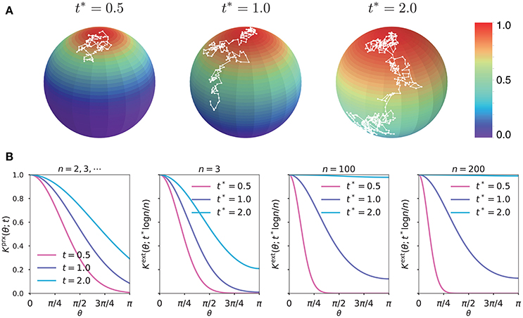
Figure 1. (A) Color maps of the exact kernel K^ext on S² at rescaled time t* = 0.5, 1.0, 2.0; the white paths are simulated random walks on S² with the Monte Carlo time approximately equal to t = t*log3/3. (B) Plots of the parametrix kernel K^prx and exact kernel K^ext on Sⁿ⁻¹, for n = 3, 100, 200, as functions of the geodesic distance.

2.3. SVM Classifications

Linear SVM seeks a separating hyperplane that maximizes the margin, i.e., the distance to the nearest data point. The primal formulation of SVM attempts to minimize the norm of the weight vector w that is normal to the separating hyperplane, subject to either hard or soft margin constraints. In the so-called Lagrange dual formulation of SVM, one applies the Representer Theorem to rewrite the weight as a linear combination of data points; in this set-up, the dot products of data points naturally appear, and kernel SVM replaces the dot product operation with a chosen kernel evaluation. The ultimate hope is that the data points will become linearly separable in the new feature space implicitly defined by the kernel.

We evaluated the performance of kernel SVM using the

1. linear kernel K^lin(x, y) = x · y,

2. Gaussian RBF K^rbf(x, y; γ) = exp{−γ|x − y|²},

3. cosine kernel $K^{\text{cos}}(\widehat{x},\widehat{y})=\widehat{x}·\widehat{y}$,

4. parametrix kernel $K^{\text{prx}}(\widehat{x},\widehat{y};t)$, and

5. exact kernel $K^{\text{ext}}(\widehat{x},\widehat{y};t)$,

on two independent data sets: (1) WebKB data of websites from four universities (WebKB-4-University) [21], and (2) glioblastoma multiforme (GBM) mutation data from The Cancer Genome Atlas (TCGA) with 5-fold cross-validations (CV) (Supplementary Material, section 1). The WebKB-4-University data contained 4,199 documents in total comprising four classes: student (1,641), faculty (1,124), course (930), and project (504); in our analysis, however, we selected an equal number of representative samples from each class, so that the training and testing sets had balanced classes. Table 1 shows the average optimal prediction accuracy scores of the five kernels for a varying number of representative samples, using 393 most frequent word features (Supplementary Material, section 1). The exact kernel outperformed the Gaussian RBF and parametrix kernel, reducing the error by 41 ~ 45% and by 1 ~ 7%, respectively. Changing the feature dimension did not affect the performance much (Table 2).

TABLE 1

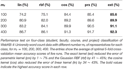
Table 1. WebKB-4-University Document Classification.

TABLE 2

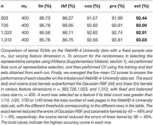
Table 2. WebKB-4-University Document Classification.

In the TCGA-GBM data, there were 497 samples, and we aimed to impute the mutation status of one gene—i.e., mutant or wild-type—from the mutation counts of other genes. For each imputation target, we first counted the number m_r of mutant samples and then selected an equal number of wild-type samples for 5-fold CV. Imputation tests were performed for top 102 imputable genes (Supplementary Material, section 1). Table 3 shows the average prediction accuracy scores for 5 biologically interesting genes known to be important for cancer [22]:

1. ZMYM4 (m_r = 33) is implicated in an antiapoptotic activity; [23, 24];

2. ADGRB3 (m_r = 37) is a brain-specific angiogenesis inhibitor [25–27];

3. NFX1 (m_r = 42) is a repressor of hTERT transcription [28] and is thought to regulate inflammatory response [29];

4. P2RX7 (m_r = 48) encodes an ATP receptor which plays a key role in restricting tumor growth and metastases [30–32];

5. COL1A2 (m_r = 61) is overexpressed in the medulloblastoma microenvironment and is a potential therapeutic target [33–35].

TABLE 3

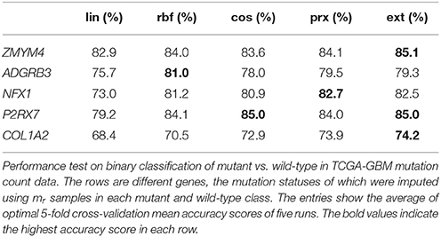
Table 3. TCGA-GBM Genotype Imputation.

For the remaining genes, the exact kernel generally outperformed the linear, cosine and parametrix kernels (Figure 2). However, even though the exact kernel dramatically outperformed the Gaussian RBF in the WebKB-4-University classification problem, the advantage of the exact kernel in this mutation analysis was not evident (Figure 2). It is possible that the radial degree of freedom $\sum _{i=1}^n{x}_i$ in this case, corresponding to the genome-wide mutation load in each sample, contained important covariate information not captured by the hyperspherical heat kernel. The difference in accuracy between the hyperspherical kernels (cos, prx, and ext) and the Euclidean kernels (lin and rbf) also hinted some weak dependence on class size m_r (Figure 2), or equivalently the sample size m = 2m_r. In fact, the level of accuracy showed much stronger correlation with the “effective sample size” $\tilde{m}$ related to the empirical Vapnik-Chervonenkis (VC) dimension [4, 7, 36–38] of a kernel SVM classifier (Figures 3A–E); moreover, the advantage of the exact kernel over the Guassian RBF kernel grew with the effective sample size ratio ${\tilde{m}}_{\text{cos}}/{\tilde{m}}_{\text{lin}}$ (Figure 3F, Supplementary Material, section 2.5.5).

FIGURE 2

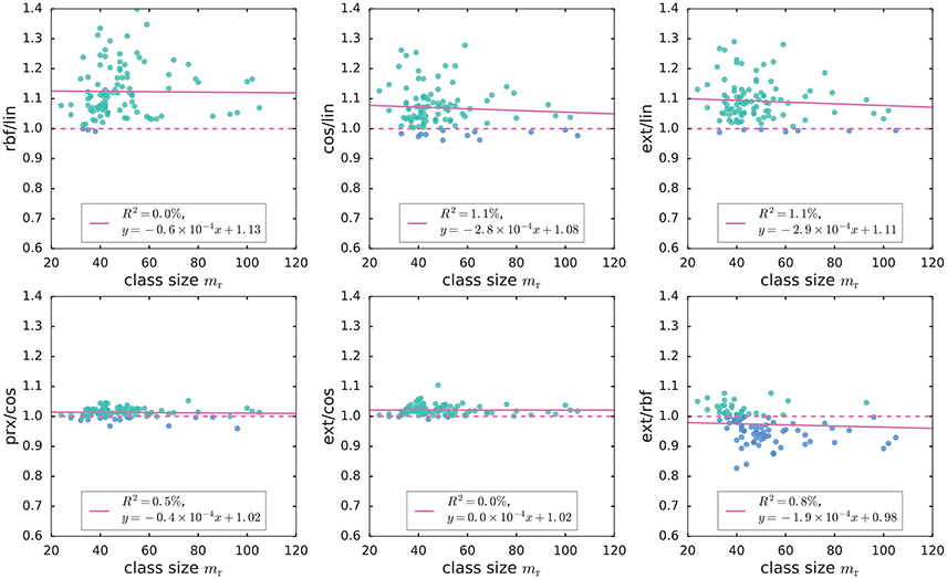
Figure 2. Comparison of the classification accuracy of SVM using linear (lin), cosine (cos), Gaussian RBF (rbf), parametrix (prx), and exact (ext) kernels on TCGA mutation count data. The plots show the ratio of accuracy scores for two different kernels. For visualization purpose, we excluded one gene with m_r = 250. The ratios rbf/lin, prx/cos, and ext/cos were essentially constant in class size m_r and greater than 1; in other words, the Gaussian RBF (rbf) kernel outperformed the linear (lin) kernel, while the exact (ext) and parametrix (prx) kernels outperformed the cosine (cos) kernel uniformly over all values of class size m_r. However, the more negative slope in the linear fit of cos/lin hints that the accuracy scores of cosine and linear kernels may depend on the class size m_r; the exact kernel also tended to outperform Gaussian RBF kernel when m_r was small.

FIGURE 3

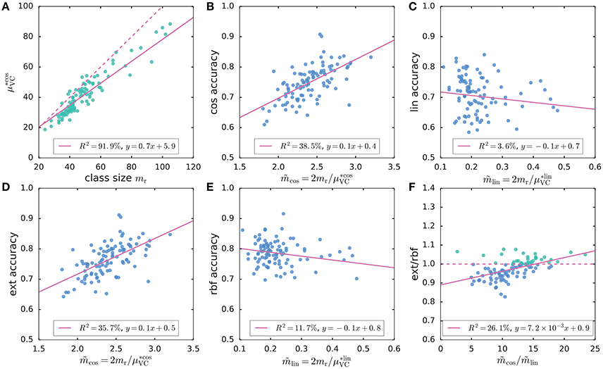
Figure 3. (A) A strong linear relation is seen between the VC-bound for cosine kernel ${\mu }_{\text{VC}}^{*cos}$ and class size m_r. The dashed line marks y = x; the VC-bound for linear kernel, however, was a constant ${\mu }_{\text{VC}}^{*\text{lin}}=439$. (B–E) The scatter plots of accuracy scores for cosine (cos), linear (lin), exact (ext), and Gaussian RBF (rbf) kernels vs. the effective sample size $\tilde{m}=2m_{\text{r}}/{\mu }_{\text{VC}}^{*}$; the accuracy scores of exact and cosine kernels increased with the effective sample size, whereas those of Gaussian RBF and linear kernels tended to decrease with the effective sample size. (F) The ratio of ext vs. rbf accuracy scores is positively correlated with the ratio ${\tilde{m}}_{\text{cos}}/{\tilde{m}}_{\text{lin}}$ of effective sample sizes.

By construction, our definition of the hyperspherical map exploits only the positive portion of the whole hypersphere, where the parametrix and exact heat kernels seem to have similar performances. However, if we allow the data set to assume negative values, i.e., the feature space is the usual ℝⁿ\{0} instead of ${ℝ}_{\ge 0}^n\backslash \{0\}$, then we may apply the usual projective map, where each vector in the Euclidean space is normalized by its L²-norm. As shown in Figure 1B, the parametrix kernel is singular at θ = π and qualitatively deviates from the exact kernel for large values of θ. Thus, when data points populate the whole hypersphere, we expect to find more significant differences in performance between the exact and parametrix kernels. For example, Table 4 shows the kernel SVM classifications of 91 S&P500 Financials stocks against 64 Information Technology stocks (m = 155) using their log-return instances between January 5, 2015 and November 18, 2016 as features. As long as the number of features was greater than sample size, n > m, the exact kernel outperformed all other kernels and reduced the error of Gaussian RBF by 29 ~ 51% and that of parametrix kernel by 17 ~ 51%.

TABLE 4

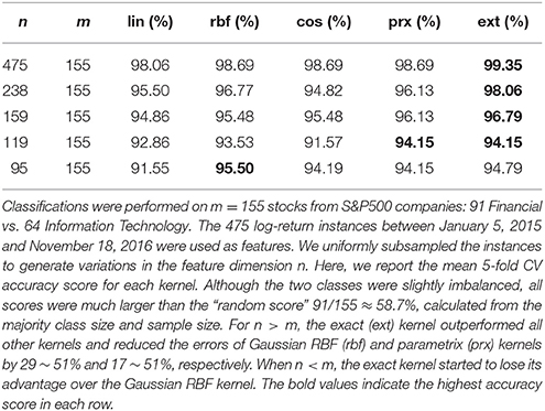
Table 4. S&P500 Stock Classification.

3. Discussion

This paper has constructed the exact hyperspherical heat kernel using the complete basis of high-dimensional angular momentum eigenfunctions and tested its performance in kernel SVM. We have shown that the exact kernel and cosine kernel, both of which employ the hyperspherical maps, often outperform the Gaussian RBF and linear kernels. The advantage of using hyperspherical kernels likely arises from the hyperspherical maps of feature space, and the exact kernel may further improve the decision boundary flexibility of the raw cosine kernel. To be specific, the hyperspherical maps remove the less informative radial degree of freedom in a nonlinear fashion and compactify the Euclidean feature space into a unit hypersphere where all data points may then be enclosed within a finite radius. By contrast, our numerical estimations using TCGA-GBM data show that for linear kernel SVM, the margin M tends to be much smaller than the data range R in order to accommodate the separation of strongly mixed data points of different class labels; as a result, the ratio R/M was much larger than that for cosine kernel SVM. This insight may be summarized by the fact that the upper bound on the empirical VC-dimension of linear kernel SVM tends to be much larger than that for cosine kernel SVM, especially in high dimensions, suggesting that the cosine kernel SVM is less sensitive to noise and more generalizable to unseen data. The exact kernel is equipped with an additional tunable hyperparameter, namely the diffusion time t, which adjusts the curvature of nonlinear decision boundary and thus adds to the advantage of hyperspherical maps. Moreover, the hyperspherical kernels often have larger effective sample sizes than their Euclidean counterparts and, thus, may be especially useful for analyzing data with a small sample size in high feature dimensions.

The failure of the parametrix expansion of heat kernel, especially in dimensions n ≫ 3, signals a dramatic difference between diffusion in a non-compact space and that on a compact manifold. It remains to be examined how these differences in diffusion process, random walk and topology between non-compact Euclidean spaces and compact manifolds like a hypersphere help improve clustering performance as supported by the results of this paper.

Author Contributions

JS conceived the project and supervised CZ who performed the calculations and analyses. CZ and JS wrote the manuscript.

Funding

This research was supported by a Distinguished Scientist Award from Sontag Foundation and the Grainger Engineering Breakthroughs Initiative.

Conflict of Interest Statement

The authors declare that the research was conducted in the absence of any commercial or financial relationships that could be construed as a potential conflict of interest.

Acknowledgments

We thank Alex Finnegan and Hu Jin for critical reading of the manuscript and helpful comments. We also thank Mohith Manjunath for his help with the TCGA data.

Supplementary Material

The Supplementary Material for this article can be found online at: https://www.frontiersin.org/articles/10.3389/fams.2018.00001/full#supplementary-material

References

1. Lafferty J, Lebanon G. Diffusion kernels on statistical manifolds. J. Mach. Learn. Res. (2005) 6:129–63.

2. Hastie T, Tibshirani R, Friedman J. The Elements of Statistical Learning. Data Mining, Inference, and Prediction. Springer Science and Business Media (2013). Available online at: http://books.google.com/books?id=yPfZBwAAQBAJ&printsec=frontcover&dq=The+elelment+of+statistical+learning&hl=&cd=4&source=gbs_api

3. Evgeniou T, Pontil M. Support vector machines: theory and applications. In: Machine Learning and Its Applications. Berlin, Heidelberg: Springer (2001). p. 249–57. Available online at: http://link.springer.com/10.1007/3-540-44673-7_12

4. Boser BE, Guyon IM, Vapnik VN. A Training Algorithm for Optimal Margin Classifiers. New York, NY: ACM (1992). Available online at: http://portal.acm.org/citation.cfm?doid=130385.130401

5. Cortes C, Vapnik V. Support-vector networks. Mach Learn. (1995) 20:273–97. doi: 10.1007/BF00994018

CrossRef Full Text

6. Freund Y, Schapire RE. Large margin classification using the perceptron algorithm. Mach Learn. (1999) 37:277–96. doi: 10.1023/A:1007662407062

CrossRef Full Text

7. Guyon I, Boser B, Vapnik V. Automatic capacity tuning of very large VC-dimension classifiers. In: Advances in Neural Information Processing Systems. (1993). p. 147–55. Available online at: https://pdfs.semanticscholar.org/4c8e/d38dff557e9c762836a8a80808c64a8dc76e.pdf

8. Kaufman L, Rousseeuw PJ. Finding groups in data. In: Kaufman L, Rousseeuw PJ, editors. An Introduction to Cluster Analysis. Hoboken, NJ: John Wiley & Sons (2009). Available online at: http://doi.wiley.com/10.1002/9780470316801.

9. Belkin M, Niyogi P, Sindhwani V. Manifold regularization: a Geometric framework for learning from labeled and unlabeled examples. J Mach Learn Res. (2006) 7:2399–434.

10. Aronszajn N. Theory of reproducing kernels. Trans Am Math Soc. (1950) 68:337. doi: 10.1090/S0002-9947-1950-0051437-7

CrossRef Full Text | Google Scholar

11. Paulsen VI, Raghupathi M. An Introduction to the Theory of Reproducing Kernel Hilbert Spaces (Cambridge Studies in Advanced Mathematics). Cambridge University Press (2016). Available online at: http://books.google.com/books?id=rEfGCwAAQBAJ&printsec=frontcover&dq=intitle:An+introduction+to+the+theory+of+reproducing+kernel+Hilbert+spaces&hl=&cd=1&source=gbs_api

Google Scholar

12. Berger M, Gauduchon P, Mazet E. Le Spectre d'une Variété Riemannienne. Springer (1971). Available online at: http://scholar.google.com/scholar?q=related:bCbU4y_3CgsJ:scholar.google.com/&hl=en&num=20&as_sdt=0,5

13. Hsu EP. Stochastic analysis on manifolds, Volume 38 of Graduate Studies in Mathematics. American Mathematical Society (2002). Available online at: http://scholar.google.com/scholar?q=related:r70JUPP2G14J:scholar.google.com/&hl=en&num=20&as_sdt=0,5.

14. Varopoulos NT,. Random Walks Brownian Motion on Manifolds. Symposia Mathematica (1987). Available online at: http://scholar.google.com/scholar?q=related:oap-nC2spI8J:scholar.google.com/&hl=en&num=20&as_sdt=0,5

15. Ng A, Jordan M, Weiss Y, Dietterich T, Becker S. Advances in Neural Information Processing Systems, 14, Chapter On spectral clustering: analysis and an algorithm (2002). Available online at: http://scholar.google.com/scholar?q=related:N4YMyham6pUJ:scholar.google.com/&hl=en&num=20&as_sdt=0,5

16. Coifman RR, Lafon S. Diffusion maps. Appl Comput Harmon Anal. (2006) 21:5–30. doi: 10.1016/j.acha.2006.04.006

CrossRef Full Text | Google Scholar

17. Atkinson K, Han W. Spherical Harmonics and Approximations on the Unit Sphere: An Introduction. Springer Science & Business Media (2012). Available online at: http://books.google.com/books?id=RnZ8SMAb6T8C&printsec=frontcover&dq=intitle:Spherical+harmonics+and+approximations+on+the+unit+sphere+an+introduction&hl=&cd=1&source=gbs_api

Google Scholar

18. Wen ZY, Avery J. Some properties of hyperspherical harmonics. J Math Phys. (1985) 26:396–9. doi: 10.1063/1.526621

CrossRef Full Text | Google Scholar

19. Stone M, Goldbart P. Mathematics for Physics: A Guided Tour for Graduate Students. Cambridge: Cambridge University Press (2009). Cambridge University Press. Available online at: http://ebooks.cambridge.org/ref/id/CBO9780511627040

Google Scholar

20. Grigor'yan A. Analytic and geometric background of recurrence and non-explosion of the Brownian motion on Riemannian manifolds. Bull Am Math Soc. (1999) 36:135–249. doi: 10.1090/S0273-0979-99-00776-4

CrossRef Full Text

21. Craven M, McCallum A, PiPasquo D, Mitchell T. Learning to extract symbolic knowledge from the World Wide Web. In: Proceedings of the National Conference on Artificial Intelligence. (1998). p. 509–16. Available online at: http://oai.dtic.mil/oai/oai?verb=getRecord&metadataPrefix=html&identifier=ADA356047

22. Hanahan D, Weinberg RA. Hallmarks of cancer: the next generation. Cell (2011) 144:646–74. doi: 10.1016/j.cell.2011.02.013

CrossRef Full Text

23. Smedley D,. SHORT COMMUNICATION Cloning Mapping of Members of the MYM Family. (1999). Available online at: http://ac.els-cdn.com/S0888754399959189/1-s2.0-S0888754399959189-main.pdf?_tid=fd1183ce-9ae9-11e6-901c-00000aacb362&acdnat=1477424224_0985e54b94244b55ec1558e901cb6211

24. Shchors K, Yehiely F, Kular RK, Kotlo KU, Brewer G, Deiss LP. Cell death inhibiting RNA (CDIR) derived from a 3'-untranslated region binds AUF1 and heat shock protein 27. J Biol Chem. (2002) 277:47061–72. doi: 10.1074/jbc.M202272200

CrossRef Full Text

25. Zohrabian VM, Nandu H, Gulati N. Gene Expression Profiling of Metastatic Brain Cancer. Oncology Reports. (2007) Available online at: https://www.spandidos-publications.com/or/18/2/321/download

26. Kaur B, Brat DJ, Calkins CC, Van, Meir EG. Brain angiogenesis inhibitor 1 is differentially expressed in normal brain and glioblastoma independently of p53 expression. Am J Pathol. (2010) 162:19–27. doi: 10.1016/S0002-9440(10)63794-7

CrossRef Full Text

27. Hamann J, Aust G, Araç, D, Engel FB, Formstone C, Fredriksson R, et al. International union of basic and clinical pharmacology. XCIV. adhesion G protein-coupled receptors. Pharmacol Rev. (2015) 67:338–67. doi: 10.1124/pr.114.009647

CrossRef Full Text

28. Yamashita S, Fujii K, Zhao C, Takagi H, Katakura Y. Involvement of the NFX1-repressor complex in PKC-δ-induced repression of hTERT transcription. J Biochem. (2016) 160:309–13. doi: 10.1093/jb/mvw038

CrossRef Full Text

29. Song Z, Krishna S, Thanos D, Strominger JL, Ono SJ. A novel cysteine-rich sequence-specific DNA-binding protein interacts with the conserved X-box motif of the human major histocompatibility complex class II genes via a repeated Cys-His domain and functions as a transcriptional repressor. J Exp Med. (1994) 180:1763–74. doi: 10.1084/jem.180.5.1763

CrossRef Full Text

30. Adinolfi E, Capece M, Franceschini A, Falzoni S. Accelerated tumor progression in mice lacking the ATP receptor P2X7. Cancer Res. (2015) 75:635–44. doi: 10.1158/0008-5472.CAN-14-1259

CrossRef Full Text

31. Gómez-Villafuertes R, García-Huerta P, Díaz-Hernández JI, Miras-Portugal MT. PI3K/Akt signaling pathway triggers P2X7 receptor expression as a pro-survival factor of neuroblastoma cells under limiting growth conditions. Nat Publ Group (2015) 5:1–15. doi: 10.1038/srep18417

CrossRef Full Text

32. Liñán-Rico A, Turco F, Ochoa-Cortes F, Harzman A, Needleman BJ, Arsenescu R, et al. Molecular signaling and dysfunction of the human reactive enteric glial cell phenotype. Inflam Bowel Dis. (2016) 22:1812–34. doi: 10.1097/MIB.0000000000000854

CrossRef Full Text

33. Anderton JA, Lindsey JC. Global analysis of the medulloblastoma epigenome identifies disease-subgroup-specific inactivation of COL1A2. Neuro Oncol. (2008) 10:981–94. doi: 10.1215/15228517-2008-048

CrossRef Full Text

34. Liang Y, Diehn M, Bollen AW, Israel MA, Gupta N. Type I collagen is overexpressed in medulloblastoma as a component of tumor microenvironment. J Neuro Oncol. (2007) 86:133–41. doi: 10.1007/s11060-007-9457-5

CrossRef Full Text

35. Schwalbe EC, Lindsey JC, Straughton D, Hogg TL, Cole M, Megahed H, et al. Rapid diagnosis of medulloblastoma molecular subgroups. Clin Cancer Res. (2011) 17:1883–1894. doi: 10.1158/1078-0432.CCR-10-2210

CrossRef Full Text

36. Vapnik VN. The Nature of Statistical Learning Theory. Springer Science & Business Media (2013). Available online at: http://books.google.com/books?id=EoDSBwAAQBAJ&printsec=frontcover&dq=intitle:The+nature+of+statistical+learning+theory&hl=&cd=1&source=gbs_api

37. Vapnik V, Levin E, Le, Cun Y. Measuring the VC-dimension of a learning machine. Neural Comput. (1994) 6:851–76. doi: 10.1162/neco.1994.6.5.851

CrossRef Full Text

38. Paliouras G, Karkaletsis V, Spyropoulos CD. Machine Learning and Its Applications. Springer (2003). Available online at: http://books.google.com/books?id=pm5rCQAAQBAJ&pg=PR4&dq=intitle:Machine+learning+and+its+applications+advanced+lectures&hl=&cd=1&source=gbs_api