Locating Decision-Making Circuits in a Heterogeneous Neural Network

Introduction

When a group of separate entities, such as ants in a colony, people in a society, or neurons in a brain, collaborate to make a decision which affects the whole group, they engage in collective decision-making. The system transitions from a state in which multiple options are possible to a state in which the system is committed to one option. This process can be broken into two separate steps: deliberation and commitment [1]. Each individual contributes to this process by both gathering information and sharing it with others. Details of these interactions differ across systems: Supreme Court members persuade one another using verbal language [2]; rock ants physically pick one another up to indicate a new preferred nesting site [3]. Determining which aspects of individual-level dynamics (for instance, the strength and density of interactions) control qualitative aspects of decision-making (for instance, the speed and consensus of the resulting decision) is key to understanding adaptive collective behavior.

A particularly well-studied example of collective decision-making comes from neuroscience. In this experimental paradigm, a monkey watches dots move on a screen and decides if more dots are moving left or right. During the task, collections of cells in the cortex accumulate information and are involved in dynamics that lead to a decision [4–6]. Spike-rate time series data taken from many neurons simultaneously has revealed that these neurons display two distinct phases during decision-making [7]. First is an aggregation phase, during which information is integrated in a distributed fashion over many neurons. Later, during a consensus phase immediately before the decision action is taken, many neurons arrive at consensus and thus redundantly encode the same information.

This binary decision-making process has been modeled in other previous work both at a very detailed level, using spiking neural models that implement attractors representing two decision states [8–10], and at a very abstract level, using one-dimensional stochastic dynamics that diffuse until they reach a preset decision boundary [11–15]. Here, we aim for a parsimonious understanding of the mechanisms that connect the dynamics of individual elements to good decision-making performance at the collective level. We therefore take a middle road between these two extremes, using a minimally complicated model amenable to analysis using dynamical systems theory, but one that still incorporates the dynamics of many individual component neurons.

Such a minimal model has been shown in previous work to explain the two phases of decision-making in terms of a transition that produces two decision state attractors [7]. Connection strengths between neurons are tuned closer to the transition during the first phase, allowing the system to slowly aggregate information from noisy sources. Moving further from the transition in the second phase allows for amplification of the decision information, leading to a strong, unambiguous decision state. In the simplest case, with identical neurons coupled all-to-all with identical connection strengths, the transition is simple to find analytically by varying a single parameter controlling the connection strength [7].

In this work, we elaborate on this previous model, identifying the transition as a symmetry-breaking pitchfork bifurcation. We use this understanding to generalize to a more realistic case, drawing on existing theory [16] to numerically locate appropriate bifurcations in a system with strong heterogeneity in interaction strengths between neurons.

We also make an analogy with statistical physics to analyze informational properties of the transition. Typically in statistical physics, microscopic dynamics are assumed to be fast enough that we can treat the system as being in equilibrium. In this case, continuous phase transitions have been shown to coincide with peaks in the Fisher Information [17–19], a generalized measure of sensitivity of a system. We develop an analogous measure of informational sensitivity that characterizes the collective properties of these dynamical, out-of-equilibrium transitions.

Methods

Neural Rate Model

A typical minimal model of neuronal activity [7, 20, 21] assumes that the state of a synapse can be represented as its membrane potential x_i ∈ ℝ and that the time derivative of x_i is the sum of external input current, leak current proportional to x_i, and input from other neurons in the system. Input from each other neuron is assumed to be proportional to its relative firing rate r_j ∈ ℝ, a dimensionless number that represents deviation from a baseline firing rate and is assumed to be a sigmoidal function of its membrane potential: r_j = g(x_j). This yields

$\begin{array}{ll}{\tau }_i\frac{d{x}_i}{dt}=I_i(t)-x_i+\xi +\frac{1}{M-1}{\displaystyle \sum _{j\ne i}}{J}_{ij}g(x_j),& (1)\end{array}$

where M is the total number of neurons, τ_i ∈ ℝ sets the timescale (in milliseconds) of the neuron returning to equilibrium in the absence of other input currents, I_i(t)/τ_i represents an external input current applied to cell i, the weights J_ij represent relative synaptic connection strengths (with units of voltage), and ξ is a Gaussian random variable representing both intrinsic synaptic noise and noise in the input I, with mean zero and variance rate Γ (with units of squared voltage per unit time). We use here g(x) = tanh(x). Example dynamics for the case of I_i(t) = 0 and homogeneous J_ij = J for all i, j is shown in Figure 1A.

FIGURE 1

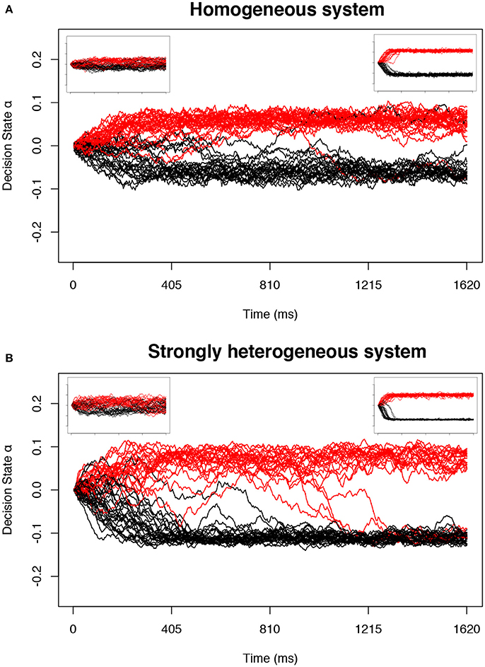
Figure 1. Example trials in the decision-making model near predicted transitions. The collective decision state of an ensemble of neurons is measured by α (Equation 17) in the stochastic model defined by Equation (1). For appropriate parameters c and a, the decision state gradually approaches one of two stable fixed point attractors as a function of time. Each simulation is plotted as one trajectory. Trajectories with positive α at the end of the stimulus (t_end = 810 ms) are interpreted as a decision for one option and colored red, and negative α as a decision for the second option and colored black. The main plot for each system shows d tuned near the point of longest-lived sensitivity; the left inset is tuned nearer to the bistable transition (d positive and small) and right inset far above the bistable transition (d positive and large). (A) The homogeneous system at the transition controlled by c alone. (B) A strongly heterogeneous system at a transition identified using our proposed method.

In the simplest case, I_i(t) = sB(t), where s ∈ ℝ is a dimensionless input signal for which positive values correspond to one of two decision states and negative values correspond to the other. We assume that the input signal is zero except between times t_start and t_end, during which it takes a constant value, making B(t) a simple boxcar function (with units of voltage). This corresponds to the typical primate experimental setup in which the relevant sensory input is presented for a limited time [4]. We set individual neuron timescales to a single typical value (τ_i = τ = 10 ms for all i) but include heterogeneity in the strengths of connection between neurons J_ij, with J_ij = c + ζ_ij where ζ_ij is a matrix of Gaussian random variables with mean zero and standard deviation γ (giving c and γ units of voltage). This moves us toward a more realistic model of individual neurons, which typically display large variance in behavior.

Our goal is to show that heterogeneity in connection strengths does not change the qualitative behavior observed in the simple homogeneous case (with γ = 0) that was proposed in Daniels et al. [7]. We expect that locating a transition in the heterogeneous case will require that we tune two parameters, since we are looking for cusp bifurcations, which are of codimension 2. We choose to vary c and a second constant input a to all neurons, which we imagine could be controlled by, for instance, neurons outside of the ones that we model. We will calculate the direction (linear combination of neurons) $\widehat{q}$ to which we expect the heterogeneous system to be most sensitive, arriving at an optimal input

$\begin{array}{ll}{I}_i(t)=a+s{q}_{i}B(t),& (2)\end{array}$

where a has units of voltage and q_i are the unitless components of the unit vector $\widehat{q}$.

The Pitchfork Bifurcation in Decision-Making

A version of the model defined in Equation (1) with homogeneous connection strengths was found to have two stable collective states when connection strengths are large enough [7]. As a model of binary decision-making, each of the two stable fixed point attractors represent a possible decision. Below a critical value of the connection strength, the two decision states merge and become indistinguishable, and near the transition, long timescales characterize dynamics between the two attractors.

In the study of nonlinear dynamics, this transition is known as a supercritical pitchfork bifurcation. At such a bifurcation, varying a control parameter causes one stable fixed point to split into three, leading to two stable fixed points on two sides of a single unstable fixed point. Pitchfork bifurcations arise more generally from “codimension 2” cusp bifurcations, in which two parameters must typically be tuned to locate the transition [16].

What is the advantage to the collective of being near such a transition instead of a bifurcation that requires tuning only one parameter? Given an existing stable fixed point, a saddle-node bifurcation can yield a second stable fixed point attractor that could be used as an alternate decision state. Yet, if only a single parameter can be varied, the two fixed points will typically be separated by fast dynamics that quickly bring the system to one state or the other, overriding slower dynamics that can gradually integrate information. This also requires that the system be separately reset to an appropriate starting value for each decision or trial. With two parameters to vary, the collective can tune to a pitchfork bifurcation that (1) contains a stable fixed point in the correct initial state that equally weights the two possible decision states in the absence of an input signal, and (2) has a slow timescale of integration near the transition.

Supercritical pitchfork transitions are analogous to continuous phase transitions in statistical physics, in which the collective state changes continuously when moving from one side of the transition to the other. In statistical physics, continuous phase transitions are understood in terms of symmetry breaking. Symmetry breaking occurs when a system transitions from inhabiting some set of collective states with equal probability (which makes the system's behavior symmetric up to a relabeling of the different states, hence the name) to inhabiting only one of those states. In the context of decision-making, symmetry breaking can be used to understand the formation of “self-organized” collective states that can represent useful information.

Procedure for Locating Pitchfork Bifurcation Parameter Values

We use the theory of bifurcations [16] to numerically locate pairs of parameter values c and a that produce pitchfork bifurcations, which have desirable properties with regard to decision-making. We start by varying $\overrightarrow{x}$ with fixed c and a to find a fixed point where the deterministic part of the dynamics are stationary in time. We then vary $\overrightarrow{x}$ and c to locate a codimension 1 bifurcation by following a curve of fixed points, and finally vary $\overrightarrow{x}$, c, and a simultaneously to locate a codimension 2 bifurcation by following a curve of codimension 1 bifurcations. This procedure is depicted graphically in Figure 2 and is described in detail below. For connections to broader dynamical systems theory, see Kuznetsov [16].

FIGURE 2

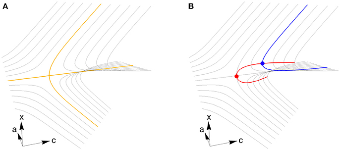
Figure 2. A cusp bifurcation and an algorithm for finding it. (A) At a supercritical pitchfork bifurcation, one stable fixed point (tracing out the yellow line to the left) splits into three fixed points (three yellow lines to the right), with two stable emerging from one unstable. The stable fixed points correspond to decision states. When a second control parameter is varied (in this case a), the fixed points vary to trace the surface that defines a cusp bifurcation (gray lines). (B) To find a codimension 1 bifurcation (blue dot), we start by varying x to find the fixed point surface, then use Equations (4–7) to follow the surface while varying x and c and keeping a fixed (blue curve). The bifurcation happens where the blue curve is vertical. To locate the codimension 2 cusp bifurcation (red dot), we start at the blue dot and use Equations (8–15) to follow the curve of codimension 1 bifurcations (red curve), allowing x, c, and a to vary. The parameter axes depicted here correspond to a system with homogeneous connectivity. Close enough to any cusp bifurcation, including those we locate in strongly heterogeneous systems, the geometry is locally equivalent to what is shown here, but is generally not aligned in the same way with respect to c and a.

Finding a Fixed Point

First, we wish to find fixed points of the deterministic part of the dynamic system in Equation (1). For ease of notation, we will call the deterministic, zero input (s = 0) part of the right hand side of Equation (1) F:

$\begin{array}{ll}{F}_i(\overrightarrow{x},c,a)\equiv a-x_i+\frac{1}{M-1}{\displaystyle \sum _{j\ne i}}{J}_{ij}g(x_j),& (3)\end{array}$

where the constant a is defined in Equation (2) and, as detailed above, J_ij = c + ζ_ij with ζ_ij a matrix of Gaussian random variables with mean zero and standard deviation γ, g(x) = tanh(x), and M is the total number of neurons. We first find a fixed point at which the set of neural states $\overrightarrow{x}$ does not change in time (with Γ = 0 and s = 0) by looking for states $\overrightarrow{x}$ at which F_i = 0 ∀ i. For a given set of model parameters c and a, we can locate fixed points numerically using a standard root-finding algorithm.

Finding a Bifurcation of Codimension 1

As we vary parameters c and a, fixed points move, and since the function F depends on these parameters in a smooth way, we can track this change along a continuous curve. Starting from one fixed point, we vary one parameter, in this case the mean neuron connection strength c, and solve for the curve along which c and $\overrightarrow{x}$ change while F remains zero. This curve is defined by

$\begin{array}{ll}\frac{d\overrightarrow{y}(\ell )}{d\ell }={\overrightarrow{v}}_y(\ell )& (4)\end{array}$

$\begin{array}{ll}{\overrightarrow{\nabla }}_y{F}_i\left(\overrightarrow{y}(\ell )\right)·{\overrightarrow{v}}_y(\ell )=0\forall i& (5)\end{array}$

$\begin{array}{ll}\left|{\overrightarrow{v}}_y(\ell )\right|=1& (6)\end{array}$

$\begin{array}{ll}\overrightarrow{y}(\ell =0)={\overrightarrow{y}}_0,& (7)\end{array}$

where $\overrightarrow{y}=\left\{x_1,x_2,\dots x_M,c\right\}$, $\overrightarrow{v}$ is the corresponding normalized velocity vector tangent to the curve, ℓ measures arclength along the curve, and the initial condition ${\overrightarrow{y}}_0$ is set at a fixed point ($F_i({\overrightarrow{y}}_0)=0\forall i$). Starting at a fixed point, we wish to perturb c and compensate by changing $\overrightarrow{x}$ in a way that keeps $F_i(\overrightarrow{y}(\ell ))=0\forall i$. This is precisely what Equation (5) accomplishes, in differential form: we choose the direction to move, ${\overrightarrow{v}}_y$, by forcing its dot product with the gradient to be zero, which keeps us on a level curve of F_i.

We find a bifurcation by following the fixed point curve defined by Equations (4–7) until the stability of the fixed point changes. A change in stability is indicated by a change in the sign of the determinant of the Jacobian, the matrix of first derivatives ${\overrightarrow{\nabla }}_x{F}_i=d{F}_i/d{x}_j$. We therefore numerically calculate the determinant as a function of ℓ along the fixed point curve and use a root-finding algorithm to locate zeros. At each corresponding codimension 1 bifurcation, we record $\overrightarrow{x}$, c, and the eigenvector of the Jacobian ${\widehat{q}}_0$ corresponding to the zero eigenvalue.

Finding a Bifurcation of Codimension 2

Starting from a bifurcation of codimension 1 that we found in the previous step, we now allow an additional parameter to vary (in this case an overall external input a) and find the curve along which $\overrightarrow{x}$, c, and a vary as the determinant of the Jacobian remains zero. To do this, we follow the same procedure as in the codimension 1 case (to keep the system at a fixed point), and in addition allow the bifurcation direction $\widehat{q}$ to vary. This constrains the system to keep the derivative along $\widehat{q}$ equal to zero:

$\begin{array}{ll}\frac{d\overrightarrow{z}(\ell )}{d\ell }={\overrightarrow{v}}_z(\ell )& (8)\end{array}$

$\begin{array}{ll}\frac{d\widehat{q}(\ell )}{d\ell }={\overrightarrow{v}}_q(\ell )& (9)\end{array}$

$\begin{array}{ll}{\overrightarrow{\nabla }}_z{F}_i\left(\overrightarrow{z}(\ell )\right)·{\overrightarrow{v}}_z(\ell )=0\forall i& (10)\end{array}$

$\begin{array}{ll}{\nabla }_{xz}^2{F}_i\left(\overrightarrow{z}(\ell )\right)·{\overrightarrow{v}}_z(\ell )·\widehat{q}(\ell )+{\overrightarrow{\nabla }}_x{F}_i\left(\overrightarrow{z}(\ell )\right)·{\overrightarrow{v}}_q(\ell )=0\forall i& (11)\end{array}$

$\begin{array}{ll}|{\overrightarrow{v}}_z(\ell )+{\overrightarrow{v}}_q(\ell )|=1& (12)\end{array}$

$\begin{array}{ll}\left|\widehat{q}(\ell )\right|=1& (13)\end{array}$

$\begin{array}{ll}\overrightarrow{z}(\ell =0)={\overrightarrow{z}}_0& (14)\end{array}$

$\begin{array}{ll}\widehat{q}(\ell =0)={\widehat{q}}_0,& (15)\end{array}$

where $\overrightarrow{z}=\left\{x_1,x_2,\dots x_M,c,a\right\}$ and the initial condition ${\overrightarrow{z}}_0$ is set at a codimension 1 bifurcation. ${\nabla }_{xz}^2$ represents the second-derivative operator $\frac{{\partial }^2}{\partial x_j\partial z_k}$.

The codimension 2 bifurcation happens when the second derivative of F with respect to $\overrightarrow{x}$ is zero along the vector $\widehat{q}$. We numerically calculate this second derivative as a function of ℓ and use a root-finding algorithm to locate zeros. We analyze the resulting codimension 2 bifurcation points to identify cusp bifurcations that produce supercritical pitchfork bifurcations as described above.

The parameter values at the resulting cusp bifurcation points ℓ* characterize each transition: $\overrightarrow{y}({\ell }^{*})$ contains the equilibrium neural states ${\overrightarrow{x}}^{*}$ and the critical parameters c* and a* at the transition; the zero mode unit vector ${\widehat{q}}^{*}$ gives the direction with which the two decision states emerge from the original single fixed point; and the two-dimensional unit vector

$\begin{array}{ll}\widehat{d}=\frac{(dc/d\ell ,da/d\ell )}{\left|(dc/d\ell ,da/d\ell )\right|}|{}_{\ell ={\ell }^{*}}& (16)\end{array}$

defines the direction in parameter space along which the pitchfork bifurcation occurs. To recover the simple homogeneous case explored in Daniels et al. [7], set ${\overrightarrow{x}}^{*}=0$, c* = 1, a* = 0, ${\widehat{q}}^{*}=\overrightarrow{1}/\left|\overrightarrow{1}\right|$ (where $\overrightarrow{1}$ is the vector of all ones, equally weighting every neuron), and $\widehat{d}=(1,0)$.

The pitchfork bifurcation can be used as a decision-making circuit by initializing the system at ${\overrightarrow{x}}_{\text{init}}={\overrightarrow{x}}^{*}$. If we vary c and a simultaneously in the direction $\widehat{d}$, such that $\overrightarrow{d}=(d_1,d_2)=d\widehat{d}$ with d having units of voltage, $c=c^{*}+d_1$, and $a=a^{*}+d_2$, then x_init is a stable fixed point when d < 0. Adjusting d then tunes the degree of bistability: small positive d corresponds to slow integration of information and larger positive d to corresponds to strong consensus.

Quantifying Decision-Making Performance

The decision-making properties of a collective of neurons tuned to a particular transition (specified by $J_{ij},a,\widehat{q},\Gamma ,$ and x_init) can be quantified by measuring both its sensitivity to the input s, the duration of that sensitivity, and the degree to which the decision state persists in time.

Collective Memory

A supercritical pitchfork bifurcation produces two stable fixed points that we consider decision states, and these fixed points emerge at ${\overrightarrow{x}}^{*}$ along the direction $\widehat{q}$. We assume that the input signal is applied along this direction in order to most effectively bias the system toward the appropriate attractor. We then identify the decision by determining whether the final neural state $\overrightarrow{x}(t_{\text{final}})$ is on the $+\widehat{q}$ or $-\widehat{q}$ side of ${\overrightarrow{x}}^{*}$. We measure distance along this dimension using the scalar decision variable

$\begin{array}{ll}\alpha =(\overrightarrow{x}-{\overrightarrow{x}}^{*})·\widehat{q},& (17)\end{array}$

so that α > 0 corresponding to one decision, and α < 0 to the other. In the case of homogeneous connection strengths, with ${\overrightarrow{x}}^{*}=0$ and $\widehat{q}\propto \overrightarrow{1}$, α is simply a rescaled version of the mean neuron state. In the heterogeneous case we must instead consider a specific linear combination $\widehat{q}$.

(We include two parenthetical remarks that could be useful in applying this analysis to real-world data. First, note that if we have increased d substantially we could potentially do better by incorporating the actual locations of the fixed points at a given d, which are only locally approximated by their values at d = 0. Second, in Daniels et al. [7], an analogous vector is found via Linear Discriminant Analysis on the neural firing data, empirically determining the most informative direction in neural firing space. Note that the experimentally measurable analog of α would be $(g(\overrightarrow{x})-g({\overrightarrow{x}}^{*}))·\widehat{v}$, where $g(\overrightarrow{x})$ represents neural firing rates. The vector $\widehat{v}$ is generally distinct from $\widehat{q}$, but could be computed in our framework. For simplicity we use $\widehat{q}$ for this paper.)

To quantify the collective memory of a system, we calculate the probability that the system is in the same decision state at time t_final as it was at the time the signal ended t_end. This measures the stability of the decision, the degree to which the system “remembers” what it has decided¹.

Collective Sensitivity

The Fisher information is particularly useful as a generalized measure of sensitivity in collective behavior [18, 19]. Fisher information can be interpreted as an information theoretic measure of the sensitivity of a system's output to its input.

In our system, we interpret the final states of neurons as the output and the stimulus as input. We are thus interested in the sensitivity of $p({\overrightarrow{x}}_{\text{final}})$(or $p({\overrightarrow{x}}_f)$) to the input stimulus s. Using notation that we explicitly define below, we want to measure $\frac{\partial }{\partial s}p({\overrightarrow{x}}_{\text{final}}|s)$. We can use the fact that the Fisher information is equal to the curvature of the KL-divergence D_KL in order to estimate it numerically:

$\begin{array}{l}\frac{\partial }{\partial s}p({\overrightarrow{x}}_f|s)\equiv -{\displaystyle \int }p({\overrightarrow{x}}_f|s)\frac{{\partial }^{2}logp({\overrightarrow{x}}_f|s)}{\partial s^2}d{\overrightarrow{x}}_f\\ ={\displaystyle \underset{\Delta s\to 0}{lim}}-{\displaystyle \int }p({\overrightarrow{x}}_f|s)\left[\frac{logp({\overrightarrow{x}}_f|s+\Delta s)-2logp({\overrightarrow{x}}_f|s_0)+logp({\overrightarrow{x}}_f|s-\Delta s)}{{(\Delta s)}^2}\right]d{\overrightarrow{x}}_f\\ ={\displaystyle \underset{\Delta s\to 0}{lim}}\frac{D_{\text{KL}}(p({\overrightarrow{x}}_f|s)||p({\overrightarrow{x}}_f|s+\Delta s))+D_{\text{KL}}(p({\overrightarrow{x}}_f|s)||p({\overrightarrow{x}}_f|s-\Delta s))}{{(\Delta s)}^2}.& (18)\end{array}$

Note that the second equality is guaranteed if $p({\overrightarrow{x}}_f|s)\frac{{\partial }^{2}logp({\overrightarrow{x}}_f|s)}{\partial s^2}$ is bounded, by the bounded convergence theorem in real analysis. While we cannot check analytically whether the function is bounded, we expect that this is true due to the smoothness of dynamics in Equation (1) and the fact that ${\overrightarrow{x}}_f$ stays bounded in our problem. Furthermore, since ${\overrightarrow{x}}_f$ is high-dimensional, it is difficult to estimate $p({\overrightarrow{x}}_f)$ directly. We instead estimate the distribution of final decision variables α. In doing this we assume that only information in the $\widehat{q}$ direction is used to make the decision. After running the simulation many times for each of three input cases (s = s₀, s₀ − Δs, and s₀ + Δs), we can estimate the resulting probability distributions over α and integrate numerically to get our desired sensitivity measure.

Results

Given a particular matrix of random connection strengths ζ_ij, we first verify that we can locate pitchfork bifurcations by varying only the two parameters c and a. By numerically solving Equations (4–7) and (8–15), we locate potentially many cusp bifurcations. Using these same equations, we trace out the locations of fixed points as a function of $\overrightarrow{d}$ (the particular linear combination of c and a defined in Equation 16) near the transition (Figure 3). These indeed display the pitchfork shape that we expect, both with weak heterogeneity (γ = 0.75), where the transition looks very similar to the homogeneous case, and with strong heterogeneity (γ = 49), where the transition appears more complicated but shares the same fundamental structure.

FIGURE 3

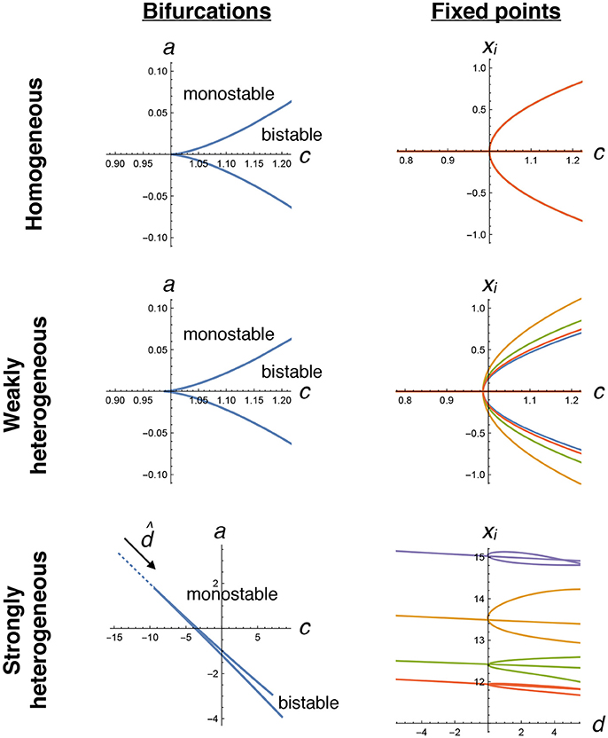
Figure 3. Pitchfork bifurcations in the decision-making model. We numerically trace the locations of bifurcations (left plots, Equations 8–15) and fixed points for four selected neurons (right plots, Equations 4–7) as a function of tuning parameters c and a. In the homogeneous case (top row), a straightforward pitchfork bifurcation happens at c = 1, with bistability that creates two stable collective states when c > 1, corresponding to positive and negative x_i values that are equal for all neurons. With weak heterogeneity, a similar transition occurs, now with each neuron having slightly different fixed point values. With strong heterogeneity, two tuning parameters need to be simultaneously varied, along the dotted line in the direction $\widehat{d}$, to find the transition. Note that each neuron's fixed point value $x_i^{*}$ can be very different. There are many possible transitions for a given ζ_ij in the strongly heterogeneous case; the one plotted here is the same example as used in other figures.

After locating these transitions, we ask whether they have the same decision-making properties that characterize the simple homogeneous-case transition. The collective properties of the system in the presence of strong noise are not analytically tractable, even in the homogeneous case, so we instead rely on numerical simulation.

First, we look at the stochastic dynamics of Equation (1) in the homogeneous case with M = 50 neurons. Example dynamics of the aggregate decision state α are shown in Figure 1A. Recapitulating the results of Daniels et al. [7], we find that the network can successfully retain collective memory of a binary decision above the transition (Figure 4A), and near the transition this information encoding is more distributed and decision dynamics happen over a longer timescale (Figures 4B,C). We extend the results of Daniels et al. [7] in the homogeneous case by showing that the collective sensitivity, measured as the Fisher information with respect to a delayed input signal, also peaks near the transition (Figure 4D).

FIGURE 4

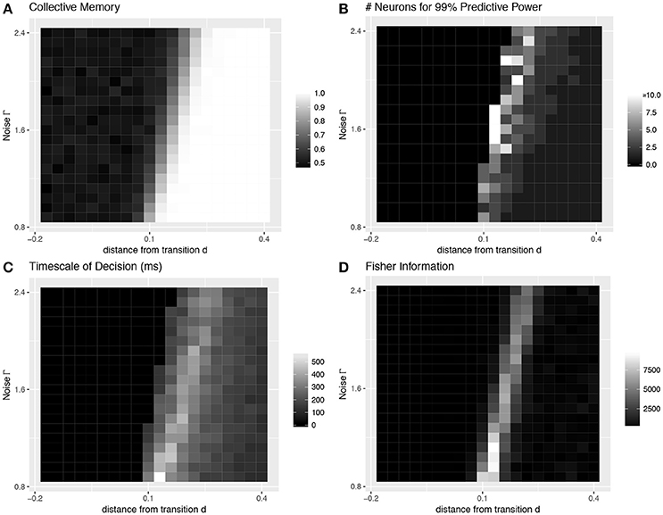
Figure 4. Collective behavior at the transition: homogeneous case. Four values characterize the collective decision-making properties of a model of neural dynamics, which we plot as a function of the distance d above a pitchfork bifurcation and the amount of noise Γ. (A) The degree of collective memory, calculated as the proportion of trials for which the final collective state correctly reflects the decision state at the end of the sensory stimulus. The system acts as a stable memory when it is far enough above the transition to bistability to overcome noise. (B) The degree to which decision information is distributed over multiple neurons peaks near the transition. Distributedness is measured by the smallest subset of neurons needed to correctly predict the same decision state to an accuracy 99% of that of the entire collective. (C) The timescale over which the decision is made, which also peaks near the transition, is measured as the time at which the entire ensemble first reaches 99% of the final predictive power. (D) The sensitivity to a perturbation applied midway through the trial (at 202.5 ms), quantified using a Fisher information measure, also peaks sharply near the transition. (A–C are a recapitulation of Figure 7 in [7]).

Most importantly, even with strong heterogeneity, we find transitions with the same decision-making properties as the simple homogeneous case (Figures 1B, 5). We again see a transition from low to high collective memory (Figure 5A), though this now requires varying two parameters (c and a) simultaneously along the vector $\overrightarrow{d}$. Near the transition, we again find that decision information is distributed over more neurons, the decision timescale is longer, and collective sensitivity is larger (Figures 5B–D).

FIGURE 5

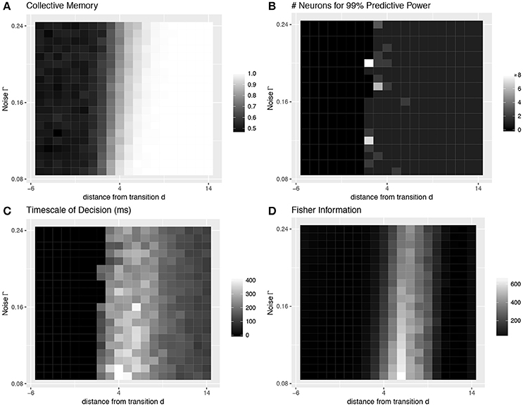
Figure 5. Collective behavior at the transition: heterogeneous case. Even with strong heterogeneity in connection strengths, we are able to locate transitions with the same decision-making properties as the simple homogeneous case in Figure 4. This figure characterizes the same heterogeneous transition depicted in the bottom row of Figure 3. See Figure 4 caption for more details.

Finally, we examine dynamical properties of our sensitivity measure. Because we initialize the system at ${\overrightarrow{x}}^{*}$, which changes in stability at the pitchfork bifurcation, we expect the sensitivity to initial perturbations to increase even as we move past the transition into the regime of strong bistability. This is intuitive: ever smaller perturbations will push the system into one of the two stable attractors when starting at an increasingly unstable fixed point. Measuring the sensitivity to delayed perturbations, we find that being near the collective transition produces the longest-lived sensitivities (Figure 6).

FIGURE 6

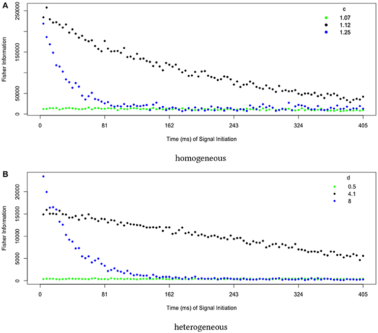
Figure 6. Collective sensitivity is longest-lived near the transition to stable memory. We quantify sensitivity using a Fisher information metric that measures how the final distribution of decision states depends on perturbations earlier in the trial. Close to the transition (green points), noise overwhelms the system and the sensitivity remains small. Far above the transition in a regime of strong bistability (blue points), small fluctuations are quickly magnified to push the system into an attractor, leaving it insensitive to perturbations applied later in the trial. At intermediate d (black points), the system remains highly sensitive over a long timescale. The behavior is qualitatively the same for transitions located in (A) homogeneous and (B) heterogeneous networks. In both figures, values are averages over 10 runs, each estimating the Fisher information using 1000 trials.

Discussion

We have developed a dynamical framework for binary decision-making that functions even in networks with highly heterogeneous connectivity. With this framework, we are able to start with a randomly-wired neural network and locate a useful transition by tuning two parameters. These parameters control the timescale over which the decision happens and the probability of falling into each decision state. The resulting circuit can be tuned by moving along a line that induces a pitchfork bifurcation. Below the bifurcation, the system maintains an uncommitted state; above but near the bifurcation, the system acts as an information integrator with timescale that depends on distance from the bifurcation; and farther from the bifurcation, the system retains a stable memory of the chosen decision.

In order to make use of such a critical transition in decision making, neural mechanisms must be capable of tuning system dynamics in specific ways that we have identified. First, two parameters must be varied to locate an appropriate bifurcation. In our example, we chose to vary the baseline constant for degree of coupling between neurons (c) and an externally-driven input into each neuron (a), which could originate from, for example, a separate set of neurons triggering a decision. We expect this framework to generalize to other pairs of tunable parameters. Second, each cusp bifurcation is associated with a specific pitchfork transition, which creates two decision states that are separated along a specific direction ${\widehat{q}}^{*}$ in state space. This means that the direction of the input signal $\widehat{q}$ needs to at least roughly match ${\widehat{q}}^{*}$ in order to perturb neurons toward the appropriate decision states.

The homogeneous version of the model in Equation (1) already recapitulates some qualitative dynamical features of observed neural decision-making dynamics [7]. Here, we have extended the analysis to a more general and more biologically realistic case by incorporating heterogeneity in connection strength between neurons. In experiments, neurons vary by orders of magnitude in both their typical firing rates and the amount of information they carry about the eventual decision [7]. The framework we present here explicitly includes these heterogeneities while remaining interpretable due to the analytical tractability of the underlying nonlinear dynamical model.

These results are linked to multiple existing frameworks in the literature of neural networks and network theory more generally. We can relate our model to Hopfield networks [22] in the limit of scaling the connection strengths J_ij to be large, or equivalently being far from the bifurcations we locate. In the Hopfield formalism, different attractors correspond to different memories; in this sense, a decision-making system might be said to be “remembering the future.” The number and stability of attractors has been extensively studied in Hopfield networks [24, 25], and is likely related to the number of potential decision bifurcation “circuits” identified by our method. In the same spirit, in the long-time equilibrium limit, our model of random interactions also shares aspects with the study of spin glasses and spin glass transitions. A variety of well-studied phase transitions in heterogeneous networks are likely related, including spin glass transitions [26] (in the long-time equilibrium limit) and percolation transitions [27, 28] (in the sense of increasing connections until consensus percolates across the entire network). Finally, our approach that starts with random connections and produces specific desired adaptive behavior shares the spirit of reservoir computing [29, 30]. The idea of constraining the behavior of a random network using a few control parameters has also been recently explored in the context of low-rank perturbations of random matrices [31].

Future empirical work will be useful to establish whether the collective sensitivity of primate cortical neurons matches with the predictions of our model. Specifically, does our Fisher information-based sensitivity measure decay as expected both as a function of time (Figure 6) and as a function of changing distance from the transition (Figure 5D)? This distance d, which we assume changes over the course of each decision process, could be estimated from the degree to which decision information is distributed over multiple neurons (using a measure similar to that shown in Figure 5B).

Our approach may also offer insight into other aspects of sensory integration, such as odor coding in the olfactory system of insects and vertebrates. In these systems, input from sensory receptor neurons must be integrated to identify specific odor sources against a noisy and variable olfactory background [32].

Beyond the brain, analyzing complicated heterogeneous dynamics by identifying specific bifurcations could be useful in the study of adaptive decision-making more generally. In the neural system discussed here, we do not expect that transmission and processing time delays produce significant effects², but they may become significant in other systems [33]. Our framework could be extended to include variation in processing and transmission time, as well as explicit heterogeneity among the individuals in the collective. During an organism's development, collective decision-making takes on an added complexity in that the developmental process actively modifies the components of the network (and thus its dynamics) at each step of the process. By incorporating such temporal effects, our approach could be made applicable to a wide variety of collective decision-making systems, such as site selection in social insect colonies and formation of quorums and biofilms in populations of microbes.

Our results add to the growing body of literature in biological collective behavior that highlight the concept of criticality and critical transitions [18, 19, 34–38, Daniels et al. in preparation]. Understanding the role such transitions play in real-world collective decision-making will be an important next step in the study of adaptive collective behavior.

Author Contributions

EA, TJ, and BD contributed to model analysis and wrote and edited the paper. BD conceptualized the research.

Conflict of Interest Statement

The authors declare that the research was conducted in the absence of any commercial or financial relationships that could be construed as a potential conflict of interest.

Acknowledgments

We thank the organizers and participants of the Data-Driven Modeling of Collective Behavior and Emergent Phenomena in Biology (DDM-Bio) Workshop, particularly Jason Graham and Simon Garnier, for providing the environment out of which this work grew. We also thank Anna Harris for helpful early discussion.

This material was based upon work partially supported by the National Science Foundation under Grant DMS-1638521 to the Statistical and Applied Mathematical Sciences Institute. Any opinions, findings, and conclusions or recommendations expressed in this material are those of the author(s) and do not necessarily reflect the views of the National Science Foundation.

Footnotes

1. ^This measure of collective memory was called “collective predictive power” in Daniels et al. [7], where the focus was on the ability of experimentally measured firing rates to predict the upcoming decision. The concept of collective memory, in which a population carries information about its past at an aggregate level, has been explored extensively in neuroscience (e.g., population codes in Hopfield networks [22]) as well as in social systems (e.g., [23]).

2. ^In the neural context, the timescale of decision-making is of the order of hundreds of milliseconds, much larger than the typical timescale of information processing of individual neurons set by τ = 10 ms, so we expect variations in τ not to qualitatively affect the dynamics. Second, neural transmission speeds are typically about 10–100 m/s, easily spanning an entire brain in the typical 10 ms neural timescale.

References

1. Gold JI, Shadlen MN. The neural basis of decision making. Annu Rev Neurosci. (2007) 30:535–74. doi: 10.1146/annurev.neuro.29.051605.113038

PubMed Abstract | CrossRef Full Text | Google Scholar

2. Lee ED, Broedersz CP, Bialek W. Statistical mechanics of the US supreme court. J Stat Phys. (2015) 160:275–301. doi: 10.1007/s10955-015-1253-6

CrossRef Full Text | Google Scholar

3. Pratt SC, Mallon EB, Sumpter DJT, Franks NR. Quorum sensing, recruitment, and collective decision-making during colony emigration by the ant Leptothorax albipennis. Behav Ecol Sociobiol. (2002) 52:117–27. doi: 10.1007/s00265-002-0487-x

CrossRef Full Text | Google Scholar

4. Shadlen MN, Newsome WT. Neural basis of a perceptual decision in the parietal cortex (area LIP) of the rhesus monkey. J Neurophysiol. (2001) 86:1916–36. doi: 10.1152/jn.2001.86.4.1916

PubMed Abstract | CrossRef Full Text | Google Scholar

5. Fetsch CR, Kiani R, Newsome WT, Shadlen MN. Effects of cortical microstimulation on confidence in a perceptual decision. Neuron (2014) 83:797–804. doi: 10.1016/j.neuron.2014.07.011

PubMed Abstract | CrossRef Full Text | Google Scholar

6. Kiani R, Cueva CJ, Reppas JB, Peixoto D, Ryu SI, Newsome WT. Natural grouping of neural responses reveals spatially segregated clusters in prearcuate cortex. Neuron (2015) 86:1–15. doi: 10.1016/j.neuron.2015.02.014

CrossRef Full Text | Google Scholar

7. Daniels BC, Flack JC, Krakauer DC. Dual coding theory explains biphasic collective computation in neural decision-making. Front Neurosci. (2017) 11:1–16. doi: 10.3389/fnins.2017.00313

PubMed Abstract | CrossRef Full Text | Google Scholar

8. Wang XJ. Probabilistic decision making by slow reverberation in cortical circuits. Neuron (2002) 36:955–68. doi: 10.1016/S0896-6273(02)01092-9

PubMed Abstract | CrossRef Full Text | Google Scholar

9. Lo CC, Wang XJ. Cortico-basal ganglia circuit mechanism for a decision threshold in reaction time tasks. Nat Neurosci. (2006) 9:956–63. doi: 10.1038/nn1722

PubMed Abstract | CrossRef Full Text | Google Scholar

10. Wang XJ. Decision making in recurrent neuronal circuits. Neuron (2008) 60:215–34. doi: 10.1016/j.neuron.2008.09.034

PubMed Abstract | CrossRef Full Text | Google Scholar

11. Usher M, McClelland JL. The time course of perceptual choice: the leaky, competing accumulator model. (2001) 108:550–92. doi: 10.1037/0033-295X.108.3.550

PubMed Abstract | CrossRef Full Text | Google Scholar

12. Ratcliff R, Smith PL. A comparison of sequential sampling models for two-choice reaction time. Psychol Rev. (2004) 111:333–67. doi: 10.1037/0033-295X.111.2.333

PubMed Abstract | CrossRef Full Text | Google Scholar

13. Ratcliff R, McKoon G. The diffusion decision model: theory and data for two-choice decision tasks. Neural Comput. (2008) 20:873–922. doi: 10.1162/neco.2008.12-06-420

PubMed Abstract | CrossRef Full Text | Google Scholar

14. Kiani R, Hanks TD, Shadlen MN. Bounded integration in parietal cortex underlies decisions even when viewing duration is dictated by the environment. J Neurosci. (2008) 28:3017–29. doi: 10.1523/JNEUROSCI.4761-07.2008

PubMed Abstract | CrossRef Full Text | Google Scholar

15. Ratcliff R, Smith PL, Brown SD, McKoon G. Diffusion decision model: current issues and history. Trends Cogn Sci. (2016) 20:260–81. doi: 10.1016/j.tics.2016.01.007

PubMed Abstract | CrossRef Full Text | Google Scholar

16. Kuznetsov YA. Elements of Applied Bifurcation Theory. New York, NY: Springer-Verlag (1995). doi: 10.1007/978-1-4757-2421-9

CrossRef Full Text | Google Scholar

17. Prokopenko M, Lizier JT, Obst O, Wang XR. Relating fisher information to order parameters. Phys Rev E (2011) 84:041116. doi: 10.1103/PhysRevE.84.041116

PubMed Abstract | CrossRef Full Text | Google Scholar

18. Daniels BC, Ellison CJ, Krakauer DC, Flack JC. Quantifying collectivity. Curr Opin Neurobiol. (2016) 37:106–13. doi: 10.1016/j.conb.2016.01.012

PubMed Abstract | CrossRef Full Text | Google Scholar

19. Daniels BC, Krakauer DC, Flack JC. Control of finite critical behaviour in a small-scale social system. Nat Commun. (2017) 8:14301. doi: 10.1038/ncomms14301

PubMed Abstract | CrossRef Full Text | Google Scholar

20. Hopfield JJ. Neurons with graded response have collective computational properties like those of two-state neurons. Proc Natl Acad Sci USA (1984) 81:3088–92. doi: 10.1073/pnas.81.10.3088

PubMed Abstract | CrossRef Full Text | Google Scholar

21. Beer RD. On the dynamics of small continuous-time recurrent neural networks. Adapt Behav. (1995) 3:469–3509. doi: 10.1177/105971239500300405

CrossRef Full Text | Google Scholar

22. Hopfield JJ. Neural networks and physical systems with emergent collective computational abilities. Proc Natl Acad Sci USA (1982) 79:2554–58. doi: 10.1073/pnas.79.8.2554

PubMed Abstract | CrossRef Full Text | Google Scholar

23. Lee ED, Daniels BC, Krakauer DC, Flack JC. Collective memory in primate conflict implied by temporal scaling collapse. J R Soc Interf. (2017) 14:20170223. doi: 10.1098/rsif.2017.0223

PubMed Abstract | CrossRef Full Text | Google Scholar

24. Amit DJ, Gutfreund H, Sompolinsky H. Spin-glass models of neural networks. Phys Rev A (1985) 32:1007–18. doi: 10.1103/PhysRevA.32.1007

PubMed Abstract | CrossRef Full Text | Google Scholar

25. Gutfreund H, Toulouse G. In: Stein DL, editor. The Physics of Neural Networks. World Scientific (1992). p. 7–59. Available online at: http://www.worldscientific.com/doi/abs/10.1142/9789814415743_0002

Google Scholar

26. Stein DL. (ed.). Spin Glasses and Biology. Singapore: World Scientific (1992).

Google Scholar

27. Stauffer D, Aharony A. Introduction to Percolation Theory. London, UK: CRC Press (1994).

Google Scholar

28. Callaway DS, Newman MEJ, Strogatz SH, Watts DJ. Network robustness and fragility: percolation on random graphs. Phys Rev Lett. (2000) 85:5468–71. doi: 10.1103/PhysRevLett.85.5468

PubMed Abstract | CrossRef Full Text | Google Scholar

29. Schrauwen B, Verstraeten D, Van Campenhout J. An overview of reservoir computing: theory, applications and implementations. In: Proceedings of the 15th European Symposium on Artificial Neural Networks. Bruges. (2007), p. 471–82.

Google Scholar

30. Sussillo D, Abbott LF. Generating coherent patterns of activity from chaotic neural networks. Neuron (2009) 63:544–57. doi: 10.1016/j.neuron.2009.07.018

PubMed Abstract | CrossRef Full Text | Google Scholar

31. Mastrogiuseppe F, Ostojic S. Linking connectivity, dynamics and computations in recurrent neural networks. (2017). arXiv 1711.09672. Available online at: http://arxiv.org/abs/1711.09672

Google Scholar

32. Pitkow X, Angelaki D. Inference in the brain: statistics flowing in redundant population codes. Neuron (2017) 94:943–53. doi: 10.1016/j.neuron.2017.05.028

PubMed Abstract | CrossRef Full Text | Google Scholar

33. Shang Y. On the delayed scaled consensus problems. Appl Sci. (2017) 7:713. doi: 10.3390/app7070713

CrossRef Full Text | Google Scholar

34. Beggs JM. The criticality hypothesis: how local cortical networks might optimize information processing. Philos Trans Ser A Math Phys Eng Sci. (2008) 366:329–43.

PubMed Abstract | Google Scholar

35. Mora T, Bialek W. Are biological systems poised at criticality? J Stat Phys. (2011) 144:268–302. doi: 10.1007/s10955-011-0229-4

CrossRef Full Text | Google Scholar

36. Beggs JM, Timme N. Being critical of criticality in the brain. Front Physiol. (2012) 3:163. doi: 10.3389/fphys.2012.00163

PubMed Abstract | CrossRef Full Text | Google Scholar

37. Cavagna A, Conti D, Creato C, Del Castello L, Giardina I, Grigera TS, et al. Dynamic scaling in natural swarms. Nat Phys. (2017) 13:914–918. doi: 10.1038/nphys4153

CrossRef Full Text | Google Scholar

38. Muñoz MA. Colloquium: criticality and dynamical scaling in living systems. arXiv 171204499 (2017).

Google Scholar