Sensor Placement for Structural Monitoring of Transmission Line Towers

Introduction

Transmission line towers form a significant part of the total cost of power transmission infrastructure. Generally, most of the transmission line towers employ steel lattice structures. Lattice towers are presently designed using traditional stress calculations obtained from linear elastic idealized truss analysis in which nodes are assumed to be concentrically loaded and members are pin connected. However, there are many discrepancies between the actual measurements obtained from full-scale prototype testing and the analytical results. Factors, such as joint eccentricity, connection rigidity, geometric and material non-linearities, uneven foundation, etc., are some of the reasons for variations in these results. Most structures are analyzed, typically using finite element software, by creating simplified models. However, real transmission line tower structures differ from idealized conditions in several aspects. Most of the lattice towers employ angle sections as members. These members that are connected with bolted connections introduce eccentricities between the line of action of the load/force and the longitudinal principal axis of the member. Zhang et al. (2013) point out that there are discrepancies in the structural behavior between the idealized model and the model with joint eccentricities included. Similarly, geometric non-linearity leads to significant differences in the displacement values (Vinay et al., 2014). Generally, truss element connections are assumed to be either pinned or rigid. However, usually semirigid connections exist (Bjorhovde et al., 1990; Kartal et al., 2010). Prasad Rao and Kalyanaraman (2001) have performed non-linear finite element analysis taking into account the effects, such as member joint eccentricity, rigidity of joints, and material non-linearity. It was found that the current methods of design based on the forces obtained from a linear analysis are not consistent with test results.

Engineers are interested in experimental results in order to determine the deviation of measured values from the predictions of analysis models. However, it may not be practical to measure the strains or deflections on each and every member. Hence, it is important to select the best locations for placing the sensors such that the real behavior of the structure is adequately explained. This issue had been investigated as early as 1978 (Shah and Udwadia, 1978). In this work, sensor placement was formulated as an optimization problem in order to minimize the error in the parameter estimates. Over the years, several methods have been proposed by various authors. Kammar and Yao (1994) proposed an iterative method called the Effective Independence method, based on the maximization of the determinant of the Fisher information matrix for optimal sensor placement. Meo and Zumpano (2005) considered the problem of locating sensors on a bridge structure with the aim of maximizing the data information so that dynamic structural behavior can be fully characterized. Some of the above techniques are developed specifically for vibration (dynamic) measurements. Vibration measurements are generally more expensive than static measurements using strain gages.

Generic sensor placement methods that can be applied to static measurements are also found in the literature. Selvaraj et al. (2013) conducted experimental analysis on the composite transmission tower using strain gages. This work did not consider the effects of modeling and measurement errors. In addition to that, uncertainties were not considered, which subsequently led to discrepancies between simulation and experimental results.

Papadimitriou (2004) addressed the theoretical and computational issues in the selection of the optimal sensor configuration for parameter estimation in structures. He proposed to quantify the uncertainty in the parameter estimates using information entropy. The concept of information entropy (H) was introduced by Shannon (1948) and is defined as

$H=-{\displaystyle {\sum }_{\text{i}}{P}_i}\left(x\right){\text{log}}_2{P}_i\left(x\right)$ (1)

where P_i(x) = probability of finding a value x within an interval i.

A uniform probability distribution gives the maximum value for the entropy. If all the values of a variable lie in the same interval, the entropy of that variable has the minimum value of 0. Hence, the entropy reflects the inhomogeneity, uncertainty, or disorder in a system. In the work of Papadimitriou (2004), among all sensor configurations, the optimal sensor configuration is selected as the one that minimizes the information entropy.

Other authors have also used entropy as a criterion for selecting optimal sensor locations. Lam et al. (2011) minimized the information entropy measure so that the uncertainty in the identification results was lower. They concluded that the top and the middle of the tower are generally good locations for sensor placement. Robert-Nicoud et al. (2005) proposed a different approach using the same concept of entropy. They chose the location and type of measurement devices such that the entropy of predictions (output variables) of candidate models is the maximum. Here, candidate models represent possible variations in the values of model parameters which are uncertain, such as support conditions and material properties. In this work, sensors are used to falsify models whose predictions do not match measurements and the approach is called “model falsification,” in order to contrast it with the optimization approach which is more common.

In the model falsification approach, the goal is to identify the candidate models that reasonably explain observations. A model is selected to be a candidate if its predictions match the measurements at each and every sensor location within the threshold of modeling and measurement errors. Measurement errors are estimated using the sensor precision data provided by manufacturers. Estimating modeling errors is more complex and involves specific knowledge about the domain (Vernay et al., 2015). The falsification process starts with generating a discrete population of model instances, which are created by randomly (or systematically) assigning values to parameters of a model class that have uncertainties. Since a large number of combinations of parameter values are possible and it is computationally expensive to evaluate each and every combination, a representative population is selected as the initially model set. The prediction of each model in the population is compared with the measurement at each sensor location and if the difference is greater than the error threshold, the model is eliminated from the set. The remaining models are accepted as the set of candidates. The process does not aim to select a single “correct” model; instead a set of models whose predictions are consistent with the measurements are selected. These models are used to predict the ranges of values of output variables at other unmeasured locations.

In order to support model falsification, the best measurement system should produce maximum separation between candidate models. The degree of separation between model predictions is evaluated using the entropy function. Maximum disorder exists when parameter values show wide dispersion. An ideal measurement system results in maximum variation in predicted responses of candidate models at the measured locations. Therefore, the location and type of measurement devices are determined such that the entropy of the set of model predictions is the maximum.

Model falsification approach has been applied to many full-scale structures details of which can be found in Goulet and Smith (2013a,b), Goulet et al. (2014), etc. This approach was also used for the analysis of wind flow around buildings using CFD by Papadopoulou et al. (2014). They replaced entropy with “joint entropy” in order to avoid selection of sensors with duplicate information content.

Wang et al. (2009) compared the performance of four existing criteria for an optimal sensor layout, namely maximum entropy of the measured variables, minimum residual entropy of the system state variables given the sensor measurements, maximum mutual information between the state variables that have not been measured and the sensor measurements; and maximum information coverage of the sensor measurements. They found out that there is no criterion that gives the best predictive results for all the environmental models tested.

Another class of methods for sensor placement uses the concept of probability updating (Beck, 2010). Flynn and Todd (2010) present a flexible sensor placement strategy within a detection theory framework, which considers the maximization of probability of detection along with minimization of costs, thus supporting decision making. They propose a Bayes risk-based performance metric to evaluate the optimal sensor configuration such that it includes both cost and detection probability. Genetic algorithm is used with one of the two criteria, i.e., either global detection rate or global false alarm rate as the fitness function to determine the best configuration. Azarbayejani et al. (2008) demonstrated a methodology to establish the probability distribution function that identifies the optimal sensor locations such that damage detection is enhanced. The approach used the weights of a neural network trained from simulations using a priori knowledge about damage locations and damage severities to generate a normalized probability distribution function for optimal sensor allocation. Even if one or more sensors fail, additional sensors are available as redundant sensors. These additional sensors were found out by computing the significant factor of each sensor and then sensors with high magnitudes are considered as critical sensors.

One of the difficulties with Bayesian updating is in estimating a priori probabilities. The results are sensitive to the probability distributions and correlations. Therefore, the model falsification approach (Robert-Nicoud et al., 2005; Goulet and Smith, 2013b) appears to be more robust. This approach is adopted in this work.

Objectives and Methodology

The overall goal of this work is to develop a generic methodology to determine optimal sensor locations for the system identification of transmission line towers. Design engineers are interested in assessing the actual stress levels in transmission line towers. However, it will be costly to place sensors on each and every member of a tower structure since transmission towers typically consist of a few hundred members and joints. Therefore, a scientific methodology for determining sensor locations is required so that the real behavior of the structure can be explained with minimum number of sensors. Since the probabilities are difficult to establish, Bayesian updating procedures are not considered for system identification. Instead, the model falsification approach is adopted and an entropy-based sensor placement strategy is used. In order to bring out the advantages of this strategy, the performance of the optimal sensor configuration is evaluated by comparing it with a traditional intuitive method. The traditional rule of thumb is to place sensors where the stresses are the maximum. In many experimental methods, this rule of thumb is followed and no systematic sensor placement method is followed. Therefore, in this work, we aim to show that the maximum stress criterion is not appropriate for identifying the best sensor locations.

The research methodology consists of the following steps:

1. Selection of a case study

2. Generation and analysis of model instances

3. Identification of optimal sensor locations using entropy-based sensor placement strategy

4. Computation of the performance metric for the optimal sensor configuration

5. Computation of the performance metric for the intuitive sensor configuration

6. Comparison of results from steps 4 and 5. These steps are described in more detail below.

Case Study

A typical 220-kV transmission tower with square base configuration is modeled (Figure 1). The structural analysis software STAAD Pro V6 was used for the analysis. Design data is summarized in Table 1. Force calculations are performed as per the Indian standard code IS 802 and one critical load combination was chosen for illustration. This loading condition involves one broken earth line resulting in asymmetric loading. The details of the loading are summarized in Table 2.

FIGURE 1

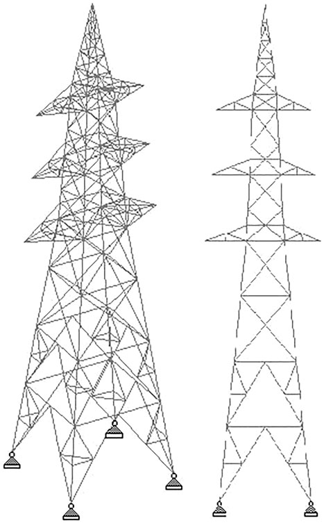
Figure 1. Views of the transmission tower selected as case study.

TABLE 1

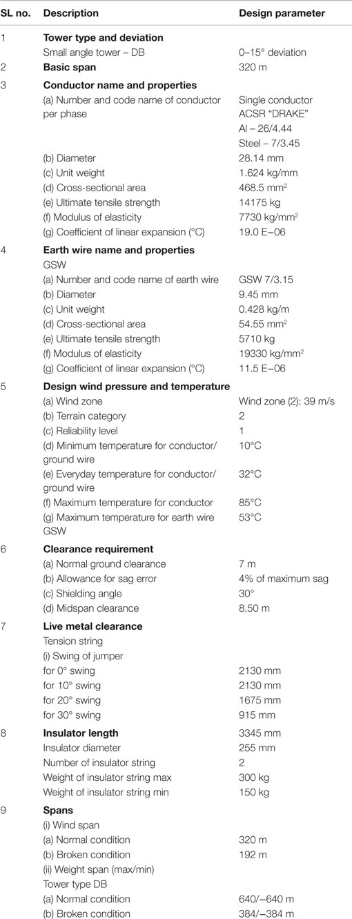
Table 1. Design data for a typical 220-kV transmission tower.

TABLE 2

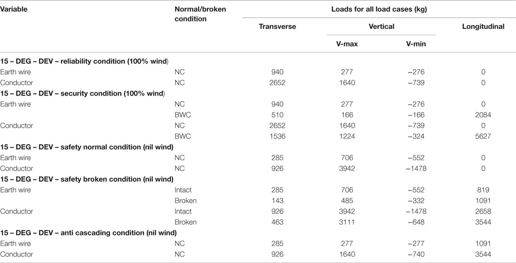
Table 2. Summary of input loading for analysis of transmission tower.

From Table 2, a load case with security loading along with earth wire broken condition is considered while conductors remain intact. Then the combination load case is formulated by considering the dead weight of the structure and the above mentioned primary load case. This combination load case is considered for the linear analysis of transmission tower. These point loads are applied at each node of six conductors and one at earth wire node accordingly.

Generation of Model Instances

Application of the model falsification approach involves generating multiple model instances by selecting different combination of values of model parameters that are uncertain. One model instance represents one set of combination of values of parameters and the corresponding results of the analysis. Linear static analysis of the transmission tower is performed. Uncertainties, such as support settlements, variations in material properties of steel, variations in joint connection rigidity, and support fixity conditions are modeled by selecting a range of values for the model parameters representing these effects. A series of model instances are generated by taking different combinations of values of these parameters as given in Table 3.

TABLE 3

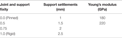
Table 3. Variables and their values for generating models.

Four conditions of connections are used, namely, pinned, rigid, and partial moment resisting connections of 50 and 75% rigidity. In a model, all the joint connections have the same fixity condition except at the supports. Assuming the same type of connections for all the joints is justified because all the connections involve similar design details and are fabricated using standard mechanized procedure. Different combinations of fixity conditions are used for the four supports. Four values of support settlements are used, namely 1, 1.5, 2, and 2.5 mm. Each value of support settlement is used for each support that is assumed to have settled. Different combinations of the four supports are assumed to have settled in different model instances. Two extreme variations of Young’s modulus for steel are used. They are 180 and 220 GPa.

By taking different combinations of the above variables, 555 model instances are generated. The model responses considered are strains in the members of the transmission line tower in the axial direction. Then for each model instance, different strain values are tabulated for different members in the tower. All the members are considered as probable locations where sensors could be placed. In total, 320 probable sensor locations are considered.

Identification of Optimal Sensor Locations

The entropy function is used to evaluate the degree of separation between the model predictions. Putting sensors at locations where model predictions have the maximum variation helps to eliminate maximum number of candidate models after a measurement is taken. Hence, sensor configuration is selected such that the entropy of the set of model predictions is the maximum. A greedy algorithm is adopted in which sensors are added one at a time based on maximum entropy. This is a variation of the joint entropy algorithm used by Papadopoulou et al. (2014). The algorithm is described in pseudocode below:

Step 1: Initialize a list to store the sensor locations that have been selected. To start with, this list is empty. Initialize a list to store sets of model instances that cannot be separated further with the current sensor configuration. To start with, the list contains a single element, which is the initial set of model instances.

Step 2: Loop over each model set i in the list of non-separable model sets.

Step 2.1: Loop over each sensor location j that has not been selected so far.

Step 2.1.1: Compute the histogram of predictions of all the models in the current set at the current sensor location.

Step 2.1.2: Compute the entropy of E(i, j) of the ith model set for the jth location.

Step 2.1.3: Move to the next sensor location and continue the loop 2.1.1.

Step 2.2: Select the next model set and continue the loop 2.1.

Step 3: Select the sensor location j with the highest entropy E(i⋅j) among all the model subsets i. Add this location to the list of selected sensor locations.

Step 4: Loop over all the sets in the list of non-separable model sets. Divide each set into subsets that cannot be separated further using the sensors that are currently selected. Remove the parent set from the list and add the subsets into the list if the number of model instances in the subset is more than one.

Step 5: If there is any more sensor location that has not been selected, repeat from Step 2.

Additional details about these steps are provided in the following sections.

Creating Histograms of Predictions

In order to compute the entropy of predictions at a given location, a histogram needs to be created. The interval width of the histogram is chosen based on this principle: when the measured value is at the midpoint of an interval, all the model predictions that are within the threshold of errors should lie within that interval. Thus, the half width of the interval is equal to the error threshold. There are errors in modeling as well as measurements. Finite element analysis does not give accurate results because of effects that are not modeled and the assumptions involved in formulating the mathematical model. Similarly, there are errors in measurements because of the precision and resolution of sensors. Hence, the error threshold is computed as the sum of the measurement and modeling errors. This is taken as the half width of the histogram.

In order to create the histogram, the range of predictions (y_min, y_max) of all the model instances at the current location is computed. This range is divided into a number of intervals using the error threshold (e) as follows:

$w=\frac{y_{\text{max}}-y_{\text{min}}}{e}$ (2)

where w is the width of the interval. The range (y_min, y_max) is divided into intervals of equal width w. Then, each model instances is assigned to one interval according to the predicted value at this location. The number of model instances that lie within an interval (N_i) is divided by the total number model instances (N) to compute the probability of the interval P_i(x) as follows:

$P_{\text{i}}\left(x\right)=\frac{N_{\text{i}}}{N}$ (3)

The probability P_i(x) is used to compute entropy as given by Eq. 1.

In order to estimate modeling errors, effects due to eccentricity and P-Delta effect are considered. Separate analysis was conducted with and without these effects and a rough estimate of modeling errors was made. Mean variation due to eccentric connections was found to be 6.73% and that due to P-Delta effect was found to be 7.05%. Measurement errors depend on the accuracy of sensors used. Here, HBM strain gage sensors are used with an accuracy of 0.1%. The total error is estimated as the sum of the absolute values of modeling and measurement errors (Vernay et al., 2015). Therefore, the error threshold is taken as 13.88%. It is emphasized that this is only a rough estimate and there are other sources of errors which have not been included. For example, there are inherent errors in the mathematical model based on Bernoulli beam hypothesis that is used to calculate the strain due to eccentric connections. Since the interval width of the histogram depends on the estimate of errors, the results are likely to be affected by the errors that are not considered. For example, if the errors are underestimated, the candidate models which are placed in adjacent intervals might be wrongly classified as separable. On the other hand, if the errors are overestimated, many candidates will be placed in the same interval and more sensors are required to separate them. The sensitivity to the error threshold is a limitation of the present work.

Dividing Model Instances into Subsets

After a sensor is chosen, the measurement from that sensor can be used to eliminate model instances whose predictions lie within other intervals. The model instances whose predictions lie within the same interval as the measurement cannot be separated with this sensor. Therefore, each set of model instances is further subdivided after a sensor is selected. Since the measured value could be within any interval, one new subset is created for each interval which contains more than one model instance. Since the initial set of model instances is hierarchically divided after each new sensor is added, this procedure automatically takes care of redundant sensor information (mutual information between sensors). That is, only those model instances that cannot be separated by the previous sensor configuration are subdivided by the new sensor. Since the entropy is calculated separately for each subset, it is conceptually the same as the joint entropy calculation used in Papadopoulou et al. (2014).

Computation of the Performance Metric

There are many possible ways of evaluating the performance of a sensor configuration. Here, the objective is to identify the state of the system. Hence, the metric chosen is the number of models that cannot be separated with the sensor configuration. An ideal configuration should be able to separate all the models and the number of non-separable models should be 0. However, this may not be possible in practice because of the low accuracy of sensors and uncertainties in modeling. In general, the number of non-separable models decreases with the addition of a new sensor. Hence, the performance of the sensor configuration can be compared only for a fixed number of sensors. The lower the number of non-separable models with a specified number of sensors, the better is the sensor configuration.

In practice, there are many other criteria that are important for selecting sensor types and their locations. Cost and feasibility of installation are important considerations. These criteria are not included in the present work.

Validation of Results

Proposed optimal sensor placement methodology is compared with the intuitive method of sensor placement, that is, by locating members having maximum stress. This comparison is performed as follows:

1. Sensors are added one by one according to the optimal sensor placement algorithm. For each configuration, the number of non-separable models is computed.

2. The locations having maximum stress are selected one by one. By placing a sensor on each of these members, the number of non-separable models using the intuitive method is computed.

3. The number of non-separable models using the two methods is compared for the same number of sensors selected.

Results

The histograms for the two locations 38 and 84 are shown in Figures 2 and 3 in order to illustrate the advantage of entropy calculations. The location 38 has the highest entropy value of 2.77 among all the locations. It can be seen that the models are fairly uniformly distributed among all the intervals. It means that once a measurement is taken, all the models in other intervals can be falsified, and it results in better identification. In contrast, at location 84 (Figure 3), most models lie within one interval. If the measured value lies within this interval (which has the highest probability), it is able to falsify only six models which are in the other intervals. The entropy at this location is close to 0, and it means that it is not a good location to place the sensor.

FIGURE 2

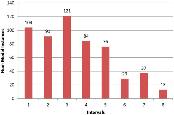
Figure 2. Frequency histogram for location 38. The prediction range at this location is divided into intervals of equal width according to the estimate of error threshold. The horizontal axis represents the interval number and the vertical axis the number of models lying in the interval.

FIGURE 3

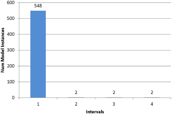
Figure 3. Frequency histogram for location 84. The prediction range at this location is divided into intervals of equal width according to the estimate of error threshold. The horizontal axis represents the interval number and the vertical axis the number of models lying in the interval.

In the first iteration of optimal sensor placement, the entropy is computed for all the locations. The first 10 locations in decreasing order of entropy are shown in Table 4.

TABLE 4

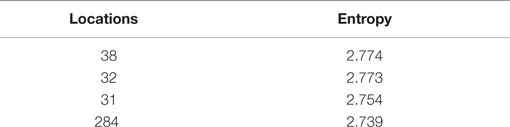
Table 4. Locations in order of decreasing entropy function.

In Table 4, location 38 has the highest entropy value of 2.774. Hence, this location is chosen as the first optimal sensor location. The above four locations are represented in the transmission tower as shown in Figure 4. All the four locations appear to be below the waist of transmission tower.

FIGURE 4

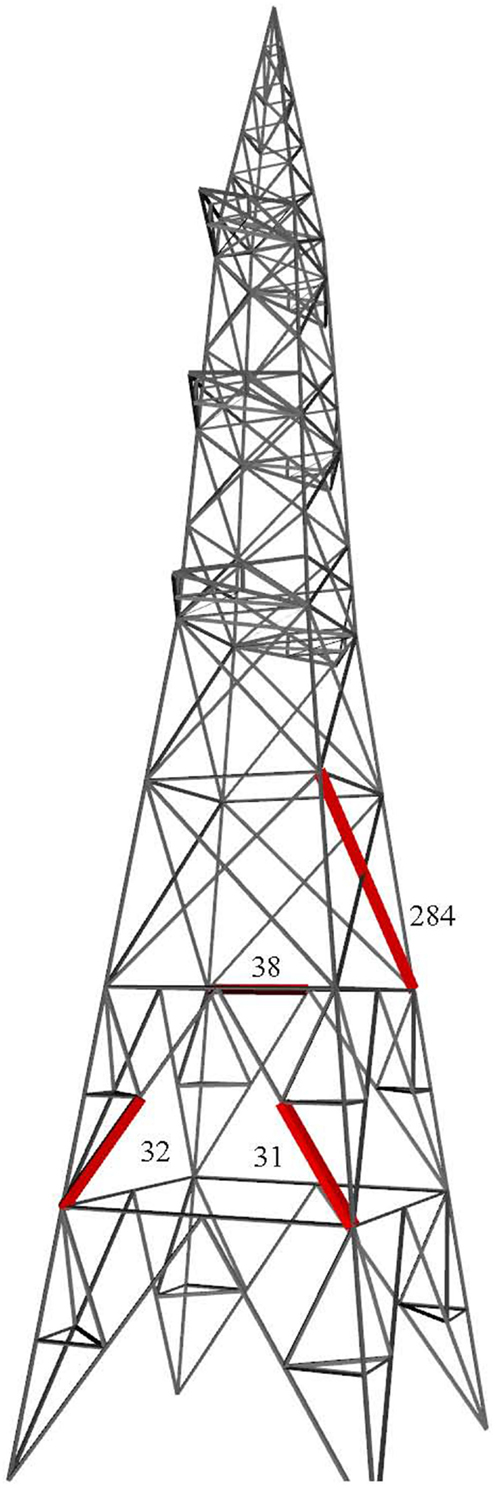
Figure 4. Locations showing first the four highest values of entropy.

Repeating the steps, the best locations selected subsequently are the members 253, 257, 201, 34, and 1. The maximum number of non-separable models decreases to two, after selecting six sensors. It does not decrease further after adding more sensors. This is summarized in Table 5 and the locations are shown in Figure 5.

TABLE 5

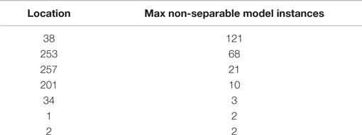
Table 5. Optimal sensor locations.

FIGURE 5

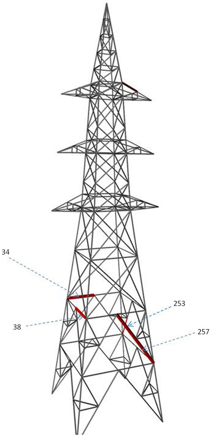
Figure 5. Optimal sensor locations.

The first three sensor locations are on the second segment of the transmission tower from the bottom. The first sensor is on a transverse bracing and the other two on a K-bracing. The fourth sensor location is at the top of the tower, where the wires are supported. The fifth sensor location is again on the second segment, where the first three sensors are located. The sixth sensor is on a leg that is connected to the foundation. This configuration of six sensors is able to separate out the model instances in the initial set such that there are at most two model instances in a subset. It should be noted that all the locations in Table 4 having highest entropy values are not selected. This is because the second location with the highest entropy duplicates information contained in the first location. The process of hierarchical separation of models automatically eliminates sensor locations with duplicate information content.

Generally, engineers would choose sensor locations by considering either maximum forces or stress values or both. Table 6 lists out the members in the ascending order of axial forces.

TABLE 6

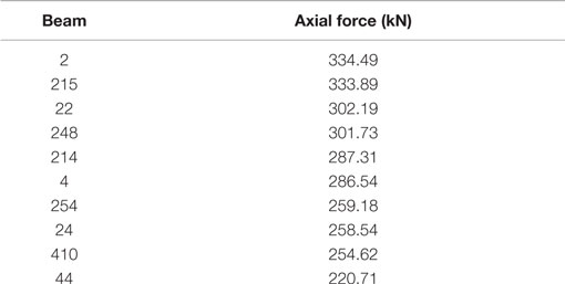
Table 6. Intuitive method of placing sensors by maximum forces.

The heavily loaded members in a transmission tower are generally leg members. Hence, when we place sensors based on maximum forces, possible locations will be at leg members as shown in Figure 6. This is completely different from the locations identified by the proposed sensor placement methodology.

FIGURE 6

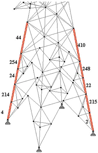
Figure 6. Intuitive method of placing sensors by maximum forces.

The performance of the intuitive method is evaluated using the metric of the maximum number of model instances that cannot be separated. It is compared with that of the optimal sensor placement methodology. For each selected number of sensors, the metrics for the two algorithms are plotted in Figure 7. It can be seen that the maximum number of non-separable models is much higher using the intuitive method compared to the optimal method. For example, with five sensors, the intuitive method results in a maximum of 13 non-separable models, while the optimal algorithm results in just three. This shows that the optimal algorithm has superior performance over the intuitive method. The gap between the two methods seems to reduce as more sensors are added. This is because some of the sensors in the optimal configuration having high model separation potential get selected at later stages of the intuitive method. However, since the intuitive method has no mechanism to detect duplicate and redundant information provided by sensors, it will require more sensors to achieve the same level of model separation.

FIGURE 7

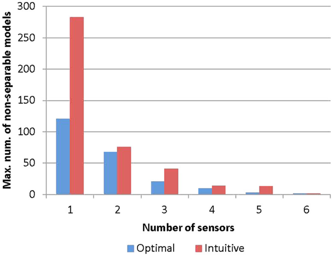
Figure 7. Maximum number of non-separable models for the two sensor placement methods.

The conclusion related to the superiority of the optimal sensor placement algorithm is based on a single case study. By repeating the study using towers with different geometries and loading conditions, the generality of the conclusion could be verified. However, it is expected that the present sensor placement strategy will have superior performance since it has firm foundations on information theory, whereas the intuitive method lacks scientific basis. Future work involves comparing the performance of other sensor placement strategies and conducting full-scale experiments to validate the results.

Summary and Conclusion

This paper presented a methodology for the placement of sensors on transmission line towers for explaining its actual structural behavior. The methodology is based on the concepts of entropy and model falsification. Sensor locations are selected based on maximum entropy such that there is maximum separation of model instances that represent different possible combinations of parameter values that are uncertain. Thus, the optimal combination of sensor locations helps to narrow down to a few possible explanations of structural behavior.

The performance of the proposed algorithm is compared to that of an intuitive method in which sensor locations are selected where the forces are maximum. It is shown that the intuitive method results in much higher number of non-separable models compared to the optimal sensor placement algorithm, especially when fewer sensors are used. The following are the specific conclusions made from the present study:

• Shannon’s entropy function is a useful tool which can identify the variability between the candidate models at possible sensor locations.

• The methodology using the entropy function provides support for sensor placement in the condition assessment of transmission towers.

• The part below the waist of the transmission tower is prone to significant variations under the considered modeling assumptions, which is evident from the fact that the top sensor locations are almost always below the waist of the tower.

• Proposed method of placing sensors helps to identify behavior models that can explain the real behavior of transmission towers, which cannot be expected from the conventional method.

• This methodology can minimize unnecessary data collection and interpretation by avoiding redundant sensors that provide no additional information.

The limitations of the present study are summarized as follows:

• Factors such as cost and ease of installation have not been included.

• The interval width of the histogram depends on estimates of modeling and measurement errors; hence, the optimality of the proposed sensor network is sensitive to the accuracy of these estimates.

• The conclusions are drawn using a single case study.

• Other sensor placement algorithms have not been compared.

• Actual experiments have not been carried out and the results are based purely on theoretical analysis.

Despite these limitations, the proposed methodology is expected to be a valuable tool to engineers in their decision-making process.

Author Contributions

The first author proposed the methodology used in the research and supervised the graduate student. The second author collected the data and performed the analysis.

Conflict of Interest Statement

The authors declare that the research was conducted in the absence of any commercial or financial relationships that could be construed as a potential conflict of interest.

Acknowledgments

The authors wish to thank the help provided by Mr. K. S. Ranjith and other colleagues at the institute.

Funding

The postgraduate study of the second author is supported by funding from Larson and Toubro (L&T).

References

Azarbayejani, M., El-Osery, A. I., Choi, K. K., and Reda Taha, M. M. (2008). A probabilistic approach for optimal sensor allocation in structural health monitoring. Smart Mater. Struct. 17, 55019. doi: 10.1088/0964-1726/17/5/055019

CrossRef Full Text | Google Scholar

Beck, J. L. (2010). Bayesian system identification based on probability logic. Struct. Contr. Health Monit. 17, 825–847. doi:10.1002/stc.424

CrossRef Full Text | Google Scholar

Bjorhovde, R., Colson, A., and Brozzetti, J. (1990). Classification system for beam to column connections. J. Struct. Eng. 116, 3059–76. doi:10.1061/(ASCE)0733-9445(1990)116:11(3059)

CrossRef Full Text | Google Scholar

Flynn, E. B., and Todd, M. D. (2010). A Bayesian approach to optimal sensor placement for structural health monitoring with application to active sensing. Mech. Syst. Signal Process. 24, 891–903. doi:10.1016/j.ymssp.2009.09.003

CrossRef Full Text | Google Scholar

Goulet, J. A., and Smith, I. F. C. (2013a). Predicting the usefulness of monitoring for identifying the behavior of structures. J. Struct. Eng. 139, 1716–1727. doi:10.1061/(ASCE)ST.1943-541X.0000577

CrossRef Full Text | Google Scholar

Goulet, J.-A., and Smith, I. F. C. (2013b). Structural identification with systematic errors and unknown uncertainty dependencies. Comput. Struct. 128, 251–258. doi:10.1016/j.compstruc.2013.07.009

CrossRef Full Text | Google Scholar

Goulet, J.-A., Texier, M., Michel, C., Smith, I. F. C., and Chouinard, L. (2014). Quantifying the effects of modeling simplifications for structural identification of bridges. J. Bridge Eng. 19, 59–71. doi:10.1061/(ASCE)BE.1943-5592.0000510

CrossRef Full Text | Google Scholar

Kammer, D. C., and Yao, L. (1994). Enhancement of on-orbit modal identification of large space structures through sensor placement. J Sound Vibration 171, 119–139.

Google Scholar

Kartal, M. E., Basaga, H. B., Bayraktar, A., and Muvafık, M. (2010). Effects of semi-rigid connection on structural responses. Electron. J. Struct. Eng. 10, 22–35.

Google Scholar

Lam, H. F., Yang, J. H., and Hu, Q. (2011). How to install sensors for structural model updating? Proc. Eng. 14, 450–459. doi:10.1016/j.proeng.2011.07.056

CrossRef Full Text | Google Scholar

Meo, M., and Zumpano, G. (2005). On the optimal sensor placement techniques for a bridge structure. Eng. Struct. 27, 1488–1497. doi:10.1016/j.engstruct.2005.03.015

CrossRef Full Text | Google Scholar

Papadimitriou, C. (2004). Optimal sensor placement methodology for parametric identification of structural systems. J. Sound Vib. 278, 923–947. doi:10.1016/j.jsv.2003.10.063

CrossRef Full Text | Google Scholar

Papadopoulou, M., Raphael, B., Smith, I., and Sekhar, C. (2014). Hierarchical sensor placement using joint entropy and the effect of modeling error. Entropy 16, 5078–5101. doi:10.3390/e16095078

CrossRef Full Text | Google Scholar

Prasad Rao, N., and Kalyanaraman, V. (2001). Non-linear behaviour of lattice panel of angle towers. J. Construct. Steel Res. 57, 1337–1357. doi:10.1016/S0143-974X(01)00054-2

CrossRef Full Text | Google Scholar

Robert-Nicoud, Y., Raphael, B., and Smith, I. F. C. (2005). Configuration of measurement systems using Shannon’s entropy function. Comput. Struct. 83, 599–612. doi:10.1016/j.compstruc.2004.11.007

CrossRef Full Text | Google Scholar

Selvaraj, M., Kulkarni, S., and Babu, R. R. (2013). Analysis and experimental testing of a built-up composite cross arm in a transmission line tower for mechanical performance. Compos. Struct. 96, 1–7. doi:10.1016/j.compstruct.2012.10.013

CrossRef Full Text | Google Scholar

Shah, P. C., and Udwadia, F. E. (1978). Methodology for optimal sensor locations for identification of dynamic systems. J. Appl. Mech. Trans. ASME. 45, 188–196. doi:10.1115/1.3424225

CrossRef Full Text | Google Scholar

Shannon, C. E. (1948). A mathematical theory of communication. Bell Syst. Tech. J. 27, 379–423. doi:10.1145/584091.584093

CrossRef Full Text | Google Scholar

Vernay, D. G., Raphael, B., and Smith, I. F. C. (2015). A model-based data-interpretation framework for improving wind predictions around buildings. J. Wind Eng. Ind. Aerod. 145, 219–228. doi:10.1016/j.jweia.2015.06.016

CrossRef Full Text | Google Scholar

Vinay, R., Ranjith, A., and Bharath, A. (2014). Optimization of transmission line towers: P-delta analysis. Eng. Technol. 3, 14563–14569.

Google Scholar

Wang, X. R., Mathews, G., Price, D., and Prokopenko, M. (2009). “Optimising sensor layouts for direct measurement of discrete variables,” in SASO 2009 – 3rd IEEE International Conference on Self-Adaptive and Self-Organizing Systems (San Francisco, CA: IEEE), 92–102.

Google Scholar

Zhang, H. W., Wang, P., and Chen, H. B. (2013). Effect of bolt slippage and joint eccentricity on the response of lattice structure with non-uniform settlement. Appl. Mech. Mater. 483, 289–296.

Google Scholar