Extended Rayleigh Damping Model

Introduction

With the recent improvements in computer performance and simulation methods, a large number of response analyses using finite element methods (FEM) with a scale of many thousands of elements have been conducted, including Onimaru et al. (2012) and Nakamura et al. (2012).

Various materials for soil and buildings were used in these analyses. This study investigated the damping models used for these materials.

In general, the internal damping of a material does not depend on the frequency. A damping model with frequency independence is called a hysteretic damping (or structural damping) model. In frequency domain analysis, a complex damping model is often used because it satisfies the condition that the damping is independent of the frequency. The complex stiffness of such a model is described as K(1 + 2h⋅i), where i is an imaginary unit, h is the damping ratio, and K is the stiffness. Therefore, h is constant with ω, as shown in Figure 1.

FIGURE 1

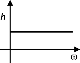
Figure 1. Complex damping model available for frequency domain analysis only.

However, this method can only be used when the entire structure is linear; it cannot be used if even a single non-linear element is present. To consider the effects of the non-linearity of a structure, time history response analyses of complete models must be performed, even if most of the elements remain in a linear condition. The objective of this study is to propose a novel damping model that can be applied to the linear elements, which are used with non-linear elements in a model.

The Rayleigh damping model is often used for such cases. This model has a mass proportional part and a stiffness proportional part. In this model, h can be defined for two frequencies, and it is approximately constant between these frequencies. This model is therefore able to express limited frequency independence. Furthermore, the computational cost of the model is small. Other formulations of damping are able to define a greater range of values of h, e.g., Chopra (2001). However, these damping matrices [C] are complete, which greatly increase the computational cost, making them seldom used.

Many recent studies have reported the effects of Rayleigh damping on inelastic response history analysis. Hall (2006) studied the problems of Rayleigh damping and noted that the damping force can become unrealistically large and the analysis response too small when during non-linear analysis softening occurs. He suggested that the causes lie in both parts. In the mass proportional part, the damping force becomes too large when the actual resonant frequencies decrease from the initial frequencies due to a reduction in stiffness. In the stiffness proportional part, when the restoring force is limited, the damping force becomes unrealistically large compared with the restoring force.

To address these problems, he proposed a capped viscous damping model that uses only a stiffness proportional damping part with an initial stiffness and a force limiter. Tangent stiffness proportional damping is not recommended because it produces a large change in the damping force and may cause convergence difficulties.

Ryan and Polanco (2008) also studied the problems of the Rayleigh damping model for a base-isolated building and recommended the use of only stiffness proportional damping.

Charney (2008) reported that excessive damping force can be created when initial stiffness is used in the non-linear condition and suggested the use of tangent stiffness instead. Zareian and Medina (2010) pointed out the same problem.

Jehel et al. (2013) compared the effect of using either initial structural stiffness or updated tangent stiffness and studied the control and design of a Rayleigh damping model. Erduran (2012) evaluated the effects of Rayleigh damping on the engineering parameters.

All these studies proposed remedies for the stiffness proportional part of Rayleigh damping. However, no remedies have been proposed for the mass proportional part, other than eliminating it altogether. This is because the frequency area where h is almost constant (hereafter referred to as the constant area) for Rayleigh damping is too narrow. Hall (2006) noted that “A small Δ (tolerance of h) and a large R (constant area where the accuracy of h is under the tolerance) are desirable, but competing goals.” If a new damping model can expand the constant area of Rayleigh damping while imposing only a small increase in the computational cost, it will provide a good solution to this problem (see Figure 2).

FIGURE 2

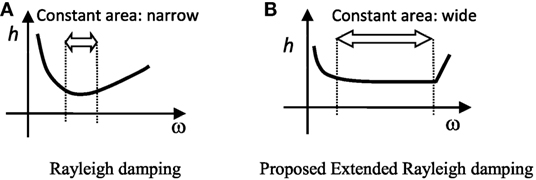
Figure 2. Damping model. (A) Rayleigh damping. (B) Proposed extended Rayleigh damping.

In an earlier study, we proposed a range of causal hysteretic damping models (hereafter referred to as a causal model), which can approximately satisfy the requirement of frequency independence (Nakamura, 2007).

In this study and based on these earlier studies, a new damping model is proposed that is able to expand the constant area by more than five times by adding two terms to the Rayleigh damping model. In this paper, the Rayleigh damping model is described, and its accuracy is discussed. Next, an outline is given of causal damping. A new model called extended Rayleigh damping is then proposed, the results of a linear analysis using this new model are reported, and its accuracy and efficiency are assessed.

Outline of the Rayleigh Model

Outline of the Model

The equation of motion can be given by Eq. 1, where [M_s], [K_s], and {u_s(t)} are, respectively, the mass matrix, stiffness matrix, and displacement vector for a structure, and {D_s(t)} is the damping vector.

$\left[M_S\right]\left\{{\ddot{u}}_S\left(t\right)\right\}+\left\{D_S\left(t\right)\right\}+\left[K_S\right]\left\{u_S\left(t\right)\right\}=\left\{0\right\}$ (1)

The Rayleigh damping model from Eq. 1 can be expressed by Eq. 2.

$\left\{D_s\left(t\right)\right\}=\left(\mathrm{\alpha }\left[M_S\right]+\mathrm{\beta }\left[K_S\right]\right)\left\{{\dot{u}}_S\left(t\right)\right\}$ (2)

Coefficients α and β are given by Eq. 3 using (ω₁, h₁) and (ω₂, h₂), where ω is the circular frequency, and h is the damping ratio.

$\mathrm{\alpha }=\frac{2{\mathrm{\omega }}_1{\mathrm{\omega }}_2\left(h_1{\mathrm{\omega }}_2-h_2{\mathrm{\omega }}_1\right)}{{\mathrm{\omega }}_2^2-{\mathrm{\omega }}_1^2},\mathrm{\beta }=\frac{2\left(h_2{\mathrm{\omega }}_2-h_1{\mathrm{\omega }}_1\right)}{{\mathrm{\omega }}_2^2-{\mathrm{\omega }}_1^2}$ (3)

As shown in Eq. 2, the Rayleigh damping model has a mass proportional part and a stiffness proportional part. The damping ratio of the former is inversely proportional to ω and that of the latter is proportional to ω. As this paper is concerned with the condition in which the damping is independent of the frequency, only the case of h_aim = h₁ = h₂, is considered, where h_aim is the target damping ratio. From this, Eq. 3 is changed to the simple form in Eq. 4.

$\mathrm{\alpha }=\frac{2h_{\text{aim}}{\mathrm{\omega }}_1{\mathrm{\omega }}_2}{{\mathrm{\omega }}_1+{\mathrm{\omega }}_2},\mathrm{\beta }=\frac{2h_{\text{aim}}}{{\mathrm{\omega }}_1+{\mathrm{\omega }}_2}$ (4)

The resulting damping ratio of the Rayleigh model has the characteristics shown in Figure 3. R_h(ω) in Eq. 5 gives the accuracy of the damping ratio h(ω) to h_aim. When ω < ω₁, R_h(ω) > 1; when ω₁ < ω < ω₂, R_h(ω) < 1; and when ω₂ < ω, R_h(ω) > 1. In Eq. 6, ω* and h* are the circular frequency and the damping ratio, respectively, when h(ω) is minimized.

$R_h\left(\mathrm{\omega }\right)=\frac{h\left(\mathrm{\omega }\right)}{h_{\text{aim}}},h\left(\mathrm{\omega }\right)=\frac{1}{2}\left(\frac{\mathrm{\alpha }}{\mathrm{\omega }}+\mathrm{\beta \omega }\right)$ (5)

${\mathrm{\omega }}^{\ast }=\sqrt{\frac{\mathrm{\alpha }}{\mathrm{\beta }}},h^{\ast }=\sqrt{\mathrm{\alpha \beta }}$ (6)

FIGURE 3

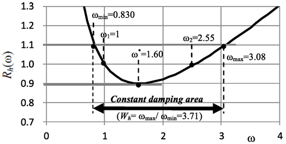
Figure 3. h(ω) of Rayleigh damping (tolerance of h = ±10% and ω₁ = 1).

Accuracy of the Rayleigh Model

The goal of this study is to propose a model that is able to realize a constant damping ratio h_aim across a wide frequency area in time history response analysis. However, in the Rayleigh damping model, only two points of ω₁ and ω₂ satisfy the requirement that h(ω) is equal to h_aim. We therefore studied the frequency area where the difference of h(ω) is within the tolerance by considering the tolerance of h(ω) against h_aim. “Tolerance,” in this case, refers to the allowable upper and lower limits from h_aim. Limits of 5 and 10% were used in this study.

Figure 3 shows R_h(ω) at a tolerance of 10%. The values for ω₁ and ω₂ were set such that the lower limit of R_h(ω) was 0.9. This figure gives each circular frequency for ω₁ as a ratio to ω = 1. Table 1 shows the values of the constant area at h_aim tolerances of 5, 10, and 20%. Here, W_h is the ratio of the maximum circular frequency ω_max to the minimum circular frequency ω_min. It can be seen that the difference in the damping ratio became less than the tolerance as W_h became larger. At tolerances of 5, 10, and 20%, the values for W_h were 2.49, 3.71, and 6.88, respectively. These values cannot be said to be satisfactory. In Hall (2006), the tolerance and W_h were notated as Δ and R, respectively, and it was observed that a small tolerance and a large W_h are desirable. However, they are competing goals for the Rayleigh model.

TABLE 1

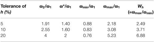
Table 1. Tolerance of damping ratio and constant area.

The resonant frequency of a structure depends on the damping ratio h(ω). The resonant frequency ω₀′ with damping is different from the undamped resonant frequency ω₀ and is expressed by Eq. 7. When the accuracy of h(ω) for h_aim is low, the accuracy of the resonant frequency also decreases. The accuracy of the resonant frequency is expressed by R_res(ω) in Eq. 8.

${\mathrm{\omega }}_0^{\prime }={\mathrm{\omega }}_0\sqrt{1-h{\left({\mathrm{\omega }}_0\right)}^2}$ (7)

$R_{\text{res}}\left(\mathrm{\omega }\right)=\sqrt{\frac{1-h{\left(\mathrm{\omega }\right)}^2}{1-{h_{\text{aim}}}^2}}$ (8)

Table 2 shows the values of R_res(ω) at a tolerance of 10%. These are the values shown in Figure 3. The values changed as h_aim changed; the values shown are for h_aim = 3, 5, and 10%. All values for R_res(ω) are 1.0 in the constant areas (ω_min ~ ω_min), so their accuracy is high.

TABLE 2

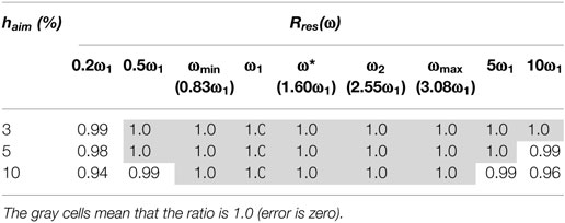
Table 2. Accuracy of resonant frequency (tolerance is 10%).

From the above, although the accuracy of R_res(ω) is high, the width W_h is small, and the accuracy of the Rayleigh damping model is unsatisfactory. A simple and practical model with a wide constant frequency area for the damping ratio is therefore desirable. This study proposed a new model, by extending the Rayleigh damping model, to expand the width W_h largely and to improve effectiveness greatly.

Outline of the Causal Model

This chapter describes the causal damping model used in this study. It is well known that the frequency-dependent function can be expressed as a series of impulses in the time domain. This Duhamel integral allows the frequency-dependent force to be expressed as the sum of the current displacement and the past displacements with each coefficient (Nakamura, 2012). “Almost frequency independent damping force” is another type of a frequency-dependent function that can be expressed in the same form.

Outline of the Model

In the complex damping model used in the frequency domain, the relationship between the reaction and displacement can be expressed by Eq. 9 in a frequency independent form, where F(ω) is the reaction, u(ω) is the displacement, K₀ is stiffness, h is the damping ratio, and i is an imaginary unit. Equation 10 is obtained by transforming Eq. 9 into the time domain. However, the calculation of I⋅u(t) is challenging.

$F\left(\mathrm{\omega }\right)=K_0\left(1+2h\cdot i\right)\cdot u\left(\mathrm{\omega }\right)$ (9)

$F\left(t\right)=K_0\left(1+2h\cdot i\right)\cdot u\left(t\right)$ (10)

Equations 11 and 12 express the unit imaginary function Z(ω) with 0 as the real part and 1 (−1 in the case of ω < 0) as the imaginary part. However, it is well known that this function is not causal and cannot be transformed into the time domain (Inaudi and Kelly, 1995).

$Z\left(\mathrm{\omega }\right)=Z_R\left(\mathrm{\omega }\right)+Z_I\left(\mathrm{\omega }\right)\cdot i$ (11)

$\begin{array}{ll}\hfill Z_R\left(\mathrm{\omega }\right)& =0,Z_I\left(\mathrm{\omega }\right)=\left\{\begin{array}{cc}1& \left(\mathrm{\omega }>0\right)\\ 0& \left(\mathrm{\omega }=0\right)\\ -1& \left(\mathrm{\omega }<0\right)\end{array}\right.\end{array}$ (12)

A number of studies on a hysteretic damping model that satisfies the causality have been carried out. For example, Inaudi and Kelly (1995) presented a precise hysteretic damping model in the tine domain based on the Hilbert transform and proposed a method for applying it to time history analyses by conducting convergent calculations. Makris (1997) proposed a causal model that can be placed at the limit of viscoelastic model of Biot (1958) and showed that this model is closer to the ideal hysteretic damping than the Biot model. Afterward, Makris and Zhang (2000) compared the model with the Biot model minutely and showed that the Biot model is more practical and reliable than the model for actual time-domain analyses. They also approximated the Biot model simply by the Prony series and showed the efficiency of the model by applying it to the response analyses of a soil structure.

Spanos and Tsavachidis (2001) proposed two methods to minimize the computational burden of the Biot model used in a time-domain analysis. One uses a recursive algorithm, and the other uses digital filters. Muscolino et al. (2005) applied the Laguerre polynomial approximation method to the Biot model in order to turn the original integrodifferential equations of motion into a set of differential equations, and the effect of the method was confirmed in both deterministic and random excitation analyses. Chouw (2002) used the causal damping model defined in the Laplace domain for the non-linear problem.

Nakamura (2007) also proposed a causal hysteretic damping model using the Hilbert transform pair and showed the high accuracy and the effectiveness of the model. In this paper, this model is used as the causal damping model.

In order to make the function causal, the real part and the imaginary part must be a Hilbert transform pair. Recalculation of the imaginary part using the Hilbert transform allows the real part [Z_k (ω)] to be obtained. It is no longer 0, but it instead becomes a frequency-dependent value [hereafter referred to as $Z_R^{\prime }\left(\mathrm{\omega }\right)$]. Z′(ω) in Eq. 13 is expressed using $Z_R^{\prime }\left(\mathrm{\omega }\right)$. We call this value, the causal unit imaginary function (Figure 4).

FIGURE 4

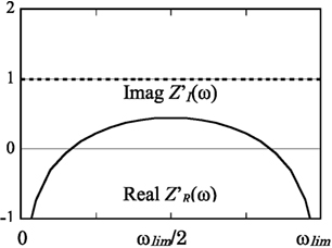
Figure 4. Calculated causal unit imaginary function Z′(ω).

The area between the upper and the lower limits (−ω_lim < ω < ω_lim, ω_lim = 2πf_lim), where the imaginary part becomes constant, must be set, allowing Eq. 9 to be approximated by Eq. 14. This area can also be expressed as 0 < f < f_lim (Hz) using f_lim (Hz) by bringing the positive frequency part into focus. Hereafter, this area is called the focused frequency area, and ω_lim and f_lim are referred to as the upper limit circular frequency and the upper limit frequency, respectively.

$Z\prime \left(\mathrm{\omega }\right)=Z_R^{\prime }\left(\mathrm{\omega }\right)+Z_I\left(\mathrm{\omega }\right)\cdot i$ (13)

$F\left(\mathrm{\omega }\right)=K_0\left(1+2h\cdot Z\prime \left(\mathrm{\omega }\right)\right)\cdot u\left(\mathrm{\omega }\right)\left(-{\mathrm{\omega }}_{\lim }<\mathrm{\omega }<{\mathrm{\omega }}_{\lim }\right)$ (14)

The causal function Z′(ω) can be transformed into the impulse response function Z′(t) in the time domain with good accuracy. This gives an approximate value for the imaginary unit i in the time domain. Equation 14 is rewritten as Eq. 15, which uses a convolution integral in the time domain.

$F\left(t\right)=K_{0}u\left(t\right)+2h{K}_0{\int }_{-\infty }^{t}Z\prime \left(t-\mathrm{\tau }\right)\cdot u\left(\mathrm{\tau }\right)d\mathrm{\tau }$ (15)

When using the time-domain transform method (Nakamura, 2006), Z′(t) is obtained as a series of discrete values. The integral from Eq. 15 is expressed by Eq. 16, where $\dot{u}\left(t\right)$ is velocity, a₀ and b_j are coefficients obtained from the time-domain transform, and Δt is 1/f_lim (s).

${\int }_{-\infty }^{t}Z\prime \left(t-\mathrm{\tau }\right)\cdot u\left(\mathrm{\tau }\right)d\mathrm{\tau }=a_0\cdot \dot{u}\left(t\right)+{\displaystyle \sum _{j=1}^N}{b}_j\cdot u\left(t-j\cdot \mathrm{\Delta }t\right)$ (16)

Equation 17 is obtained by substituting Eq. 16 into Eq. 15. This is the target equation in the time domain. The first term on the right side of this equation corresponds to the ordinary restoring force, and the second term corresponds to the damping force. As a result, the reaction F(t) at the current time t is expressed as the sum of the coefficient products of the current displacement u(t), the current velocity $\dot{u}\left(t\right)$, and past displacements u(t − j⋅Δt).

$F\left(t\right)=K_{0}u\left(t\right)+2h{K}_0\left(a_0\cdot \dot{u}\left(t\right)+{\displaystyle \sum _{j=1}^N}{b}_j\cdot u\left(t-j\cdot \mathrm{\Delta }t\right)\right)$ (17)

In the frequency domain, Z′(ω) can be expressed by Eq. 18 using a₀ and b_j. F(ω) can be calculated by substituting Z′(ω) into Eq. 14.

$Z\prime \left(\mathrm{\omega }\right)=i\mathrm{\omega }\cdot a_0+{\displaystyle \sum _{j=1}^N}{b}_j\cdot e^{-i\mathrm{\omega }\cdot j\cdot \mathrm{\Delta }t}$ (18)

Equation 17 is rewritten as Eq. 19, where {F_E(t)}, {u_E(t)}, and [K_E] are the element reaction vector, the element displacement vector, and the element stiffness matrix, respectively. This causal model is clearly independent of the element type, and different types of element can be employed in the same way.

$\left\{F_E\left(t\right)\right\}=\left[K_E\right]\left\{u_E\left(t\right)\right\}+2h\left[K_E\right]\cdot \left(a_0\cdot \left\{{\dot{u}}_E\left(t\right)\right\}+{\displaystyle \sum _{j=1}^N}{b}_j\cdot \left\{u_E\left(t-j\cdot \mathrm{\Delta }t\right)\right\}\right)$ (19)

Nakamura (2008) proposed a method for simultaneously calculating the real part and the impulse response in the time domain with only the imaginary part of the complex function. This was done using the Kramers–Kroning relation (Nakamura, 2007). This process also provided a method for obtaining Z′(t) by carrying out time-domain transform directly, using only the imaginary part Z_I (ω) and without conducting the numerical Hilbert transform. This method yields a model with higher accuracy because the omission of the numerical Hilbert transform reduces the calculation error. This model was used in the current study.

Equation 20 was obtained by expressing Eq. 19 as the damping force vector {D_S (t)} of Eq. 1 (the equation of motion). In this equation, the stiffness proportional model with coefficient β of the first term is modified by the sum of the coefficient product terms of the past displacement of the second term (hereafter referred to as the time delay part term). Equation 21 shows the corresponding damping vector {D_S (ω)} in the frequency domain.

$\begin{array}{llll}\hfill \left\{D_s\left(t\right)\right\}& =2h\left[K_S\right]\cdot \left(a_0\cdot \left\{{\dot{u}}_S\left(t\right)\right\}+{\displaystyle \sum _{j=1}^N}{b}_j\left\{u_S\left(t-j\cdot \mathrm{\Delta }t\right)\right\}\right)& & \\ & =\mathrm{\beta }\left[K_S\right]\left\{{\dot{u}}_S\left(t\right)\right\}+2h\left[K_S\right]\cdot \left({\displaystyle \sum _{j=1}^N}{b}_j\left\{u_S\left(t-j\cdot \mathrm{\Delta }t\right)\right\}\right)\end{array}$ (20)

where $\mathrm{\beta }=2h{a}_0=\frac{4h}{{\mathrm{\omega }}_{\lim }}=\frac{2h}{\mathrm{\pi }\cdot f_{\lim }}$.

$\left\{D_s\left(\mathrm{\omega }\right)\right\}=\left(i\mathrm{\omega }\cdot \mathrm{\beta }+2h\cdot {\displaystyle \sum _{j=1}^N}{b}_j\cdot e^{-i\mathrm{\omega }\cdot j\cdot \mathrm{\Delta }t}\right)\cdot \left[K_S\right]\left\{u_S\left(\mathrm{\omega }\right)\right\}$ (21)

Figure 5A shows an image of the causal damping model. In the frequency area considered (0 ~ ω_lim), the damping ratio h(ω) is almost constant. However, the characteristics are different at the two ends of the area, as h(ω) changes from 0 to h_aim in the vicinity of ω = 0, and from h_aim to 2h_aim near ω = ω_lim. This model is calculated as the sum of the stiffness proportional damping part with h_aim at ω_lim/2, shown in Figure 5B, and the term of the time delay part, shown in Figure 5C. The former corresponds to the first term Eq. 20, and the latter corresponds to the second term.

FIGURE 5

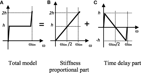
Figure 5. Causal damping model. (A) Total model. (B) Stiffness proportional part. (C) Time delay part.

Figure 6 includes the outside of ω_lim. The causal model can be regarded as being made by changing the stiffness proportional part of the Rayleigh damping model to a step form.

FIGURE 6

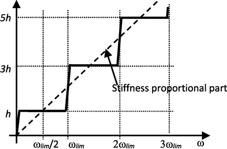
Figure 6. Image of causal damping model with the area greater than ω_lim.

Coefficients and Characteristics of Representative Models

Table 3 shows the coefficients (a₀ and b_j) of representative cases, where ω_lim is the upper limit circular frequency for the 9-term, 4-term, and 2-term models. The models are identified by the time delay part b_j, and are labeled the C9, C4, and C2 models. Models with a higher number are more accurate. The value of a₀ for all the models is the same as 1/(πf_lim), and Δt is 1/f_lim(s).

TABLE 3

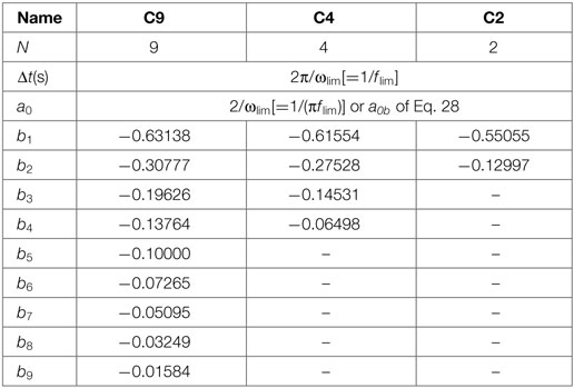
Table 3. Coefficients of the causal damping model.

Table 4 describes the condition of each model in the time-domain transform. The “frequencies used for transform” of each model are expressed as 0 ~ 1 (normalized with ω_lim). In this frequency area, the time-domain transform requires that the imaginary part become 1, and the imaginary part is interpolated smoothly.

TABLE 4

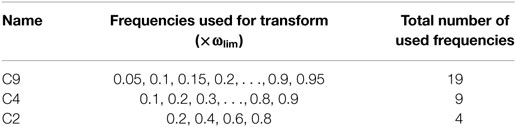
Table 4. Conditions of time-domain transform.

Although Δt does not need to agree with the time step ΔT for a time history response analysis, Δt should be an integer multiple of ΔT. For example, at values of 0.1 s for Δt and 0.01 s for ΔT, the values at every 10 steps of the results obtained from the response analyses need to be used to derive the past displacement vector {u_s(t − jΔt)}. If ΔT is changed in the analysis, it is unnecessary to change Δt.

Figure 7 compares the Z′(ω) of each model. This figure was obtained by transforming the coefficients in Table 3, which were obtained from the transform to the time domain, back to the frequency domain. The values of the imaginary parts of all models are 1 at the frequencies used for the transform shown in Table 4. Accordingly, the area in which the value of the imaginary part is close to 1 is 0.05ω_lim ~ 0.95ω_lim for the C9 model and 0.2ω_lim ~ 0.8ω_lim for the C2 model.

FIGURE 7

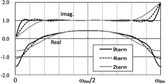
Figure 7. Comparison of Z′(ω) values.

In the real part, the maximum values at ω_lim/2 are almost the same across all models. However, near the ends (0 or ω_lim), the value for the C9 model decreases sharply, while that of the C2 model decreases more slowly.

We next addressed the accuracy of K₀ (1 + 2hZ′(ω)), when this Z′(ω) was used. Since the target complex stiffness in the frequency domain was K₀ (1 + 2hi), 1 + 2hZ′(ω) was compared with the target value 1 + 2hi.

The damping ratio of the causal model, h′(ω), was obtained by Eq. 22 using the ratio of the imaginary part to the real part of 1 + 2hZ′(ω) (Nakamura, 2007).

The accuracy R_h(ω) for the target damping ratio h_aim was calculated using Eq. 23.

$h\prime \left(\mathrm{\omega }\right)=\sin \left(\frac{1}{2}{\tan }^{-1}\frac{2h_{\text{aim}}\cdot Z_I^{\prime }\left(\mathrm{\omega }\right)}{1+2h_{\text{aim}}\cdot Z_R^{\prime }\left(\mathrm{\omega }\right)}\right)$ (22)

$R_h\left(\mathrm{\omega }\right)=\frac{h\prime \left(\mathrm{\omega }\right)}{h_{\text{aim}}}$ (23)

Figure 8 shows the R_h(ω) of the C9 and C2 models. In this figure, R_h(ω) when h_aim = 1, 3, 5, and 10 is shown because it changes as h_aim changes.

FIGURE 8

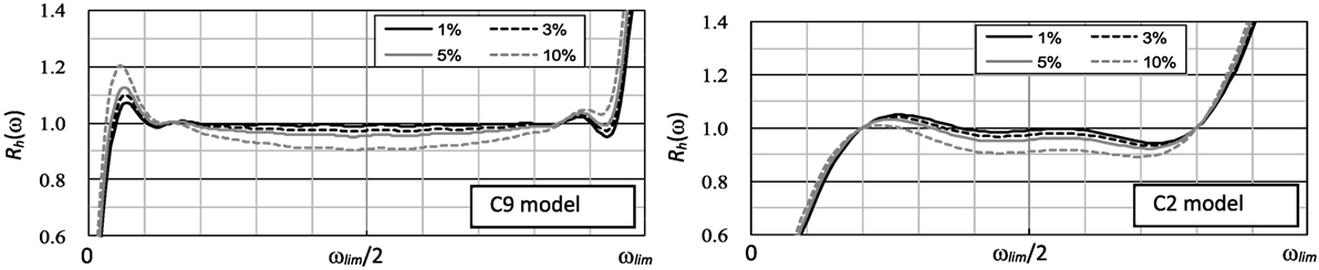
Figure 8. Accuracy of the damping ratio R_h(ω) when h_aim = 1, 3, 5, and 10%.

Overall, the shapes of R_h(ω) resembled those of $Z_I^{\prime }$(ω). When h_aim was small, the accuracy tended to be high, and R_h(ω) was therefore close to 1.

Next, a comparison between the C9 and C2 models was carried out, and the accuracy of the C9 model was shown to be higher overall, with a value of R_h(ω) close to 1 in the area between 0.1ω_lim and 0.9ω_lim, whereas that of the C2 model was close to 1 in the area between 0.2ω_lim and 0.8ω_lim. The accuracy of R_h(ω) in the C9 model decreased locally at both ends of the area. This became more notable as the value of h_aim increased. In contrast, this tendency was hardly observed in the C2 model. These characteristics are produced by the shapes of $Z_I^{\prime }\left(\mathrm{\omega }\right)$ at the ends of the frequency area.

Furthermore, when the value of h_aim was large, the accuracy value was less than 1 across a wide frequency area because of the comparatively large value of $Z_R^{\prime }\left(\mathrm{\omega }\right)$ in the central region.

The accuracy of the resonant frequency R_res(ω) of the causal model was then investigated. R_res(ω) was calculated using Eq. 24, obtained by multiplying the value of Eq. 25 by Eq. 8.

$R_{\mathit{res}}\left(\mathrm{\omega }\right)=\frac{{\mathrm{\omega }}_0\left(\mathrm{\omega }\right)}{{\mathrm{\omega }}_0}\sqrt{\frac{1-h\prime \left(\mathrm{\omega }\right)2}{1-{h_{\text{aim}}}^2}}$ (24)

$\frac{{\mathrm{\omega }}_0\left(\mathrm{\omega }\right)}{{\mathrm{\omega }}_0}=\sqrt{1+2h_{\text{aim}}\cdot Z_R^{\prime }\left(\mathrm{\omega }\right)}$ (25)

Figure 9 shows the values of R_res(ω) in the C9 and C2 models. The shapes of R_res(ω) resembled those of $Z_R^{\prime }\left(\mathrm{\omega }\right)$. The accuracy became higher as the value of h_aim decreased. Across all models, when h_aim was large, R_res(ω) was greater than 1 in the central part of the frequency area around ω_lim/2. In contrast, R_res(ω) tended to fall below 1 at both ends of the frequency area. In the C9 model, this decrease in R_res(ω) was significant, whereas the reduction in accuracy in the C2 model was relatively small. This reflected the shapes of $Z_R^{\prime }\left(\mathrm{\omega }\right)$.

FIGURE 9

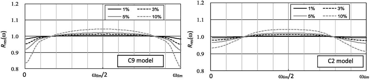
Figure 9. Accuracy of the resonant frequency R_res(ω) when h_aim = 1, 3, 5, and 10%.

Improvement of the Causal Model

This decrease in accuracy R_h(ω) area around ω_lim/2 when h_aim is large was addressed next.

Figure 10 gives an outline of the modification method. Figure 10A shows the hollow on the low-frequency side from the center being supplemented by the stiffness proportional damping. As a result, the accuracy decreases slightly on the high-frequency side from the center of the focused frequency area. The damping ratio h′(ω), which is obtained by a response analysis for the target damping ratio h_aim, can be approximated using Eq. 26. At the central part of the frequency area where the accuracy is lowest, $Z_I^{\prime }\left({\mathrm{\omega }}_{\lim }∕2\right)$ becomes a₀⋅(ω_lim/2). Then, a₀ is increased $\left(1+2h_{\text{aim}}\cdot Z_I^{\prime }\left({\mathrm{\omega }}_{\lim }∕2\right)\right)$ times. A new value for a₀ (assuming a_0a) is used in Eq. 27, with a₀ = 1/(πf_lim). Table 5 shows the $Z_R^{\prime }\left({\mathrm{\omega }}_{\lim }∕2\right)$ value in each model. When h_aim is large, an error arises from the difference between Eqs 22 and 26.

FIGURE 10

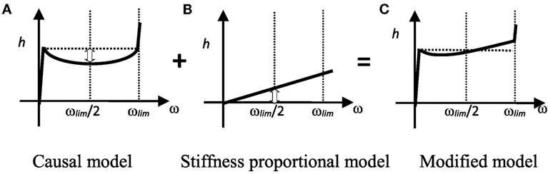
Figure 10. Modification 2 (addition of stiffness proportional damping). (A) Causal model. (B) Stiffness proportional model. (C) Modified model.

TABLE 5

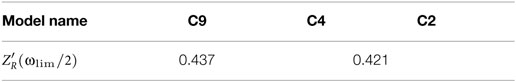
Table 5. ${\mathit{\text{Z}}}_{\mathit{\text{R}}}^{\prime }\left({\mathrm{\omega }}_{\mathbf{\text{lim}}∕2}\right)$ for each model.

From a practical point of view, the use of a₀ (assuming a_0b) from Eq. 28 is recommended. This equation is obtained by correcting the difference using a quadratic expression for h_aim. In the numerical study, cases where h_aim was less than or equal to 10% were investigated. From the results, 1.5 and 3.7 were selected as optimum coefficients.

Figure 11 shows R_h(ω) calculated using a_0b for the C9 and C2 models. Since R_h(ω_lim/2) was almost 1, the effect of the correction was confirmed. This correction has little effect on R_res(ω).

$h\prime \left(\mathrm{\omega }\right)\approx \frac{h_{\text{aim}}\cdot Z_I^{\prime }\left(\mathrm{\omega }\right)}{1+2h_{\text{aim}}\cdot Z_R^{\prime }\left(\mathrm{\omega }\right)}$ (26)

$a_{0a}=\frac{1+2h_{\text{aim}}{Z}_R^{\prime }\left({\mathrm{\omega }}_{\lim }∕2\right)}{{\mathrm{\omega }}_{\lim }∕2}=a_0+\frac{4h_{\text{aim}}{Z}_R^{\prime }\left({\mathrm{\omega }}_{\lim }∕2\right)}{{\mathrm{\omega }}_{\lim }}$ (27)

$a_{0b}=a_0+\left(1+1.5h_{\text{aim}}+3.7h_{\text{aim}}^2\right)\cdot \frac{4h_{\text{aim}}{Z}_R^{\prime }\left({\mathrm{\omega }}_{\lim }∕2\right)}{{\mathrm{\omega }}_{\lim }}$ (28)

FIGURE 11

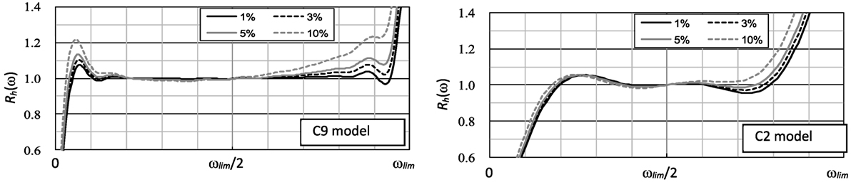
Figure 11. Accuracy of the damping ratio R_h(ω).

Proposal for a New Model

As noted above, the Rayleigh model is simple and effective, but the frequency area in which the damping ratio can be regarded as constant is narrow. In this section, we propose a novel model, which has a wide constant frequency area.

Outline of the Proposed Model

Rayleigh damping is a combination of mass proportional damping and stiffness proportional damping, as illustrated in Figure 12. In our new model, the stiffness proportional damping is replaced by causal damping (Figure 13). The damping ratio h′(ω) can be approximated by Eq. 29 using Eqs 5 and 26. This allows the constant frequency area to be expanded. Therefore, the new model can be thought of as adding Rayleigh damping to the time delay term.

$h\prime \left(\mathrm{\omega }\right)\approx \frac{\mathrm{\alpha }}{\mathrm{2\omega }}+\frac{h_{\text{aim}}\cdot Z_I^{\prime }\left(\mathrm{\omega }\right)}{1+2h_{\text{aim}}\cdot Z_R^{\prime }\left(\mathrm{\omega }\right)}$ (29)

FIGURE 12

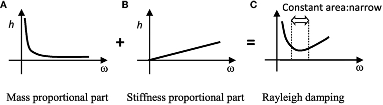
Figure 12. Rayleigh damping. (A) Mass proportional part. (B) Stiffness proportional part. (C) Rayleigh damping.

FIGURE 13

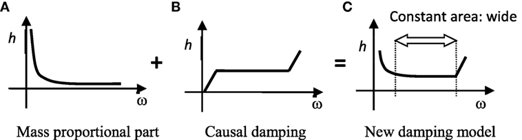
Figure 13. New damping model. (A) Mass proportional part. (B) Causal damping. (C) New damping model.

The new model was constructed as follows:

1) In the constant frequency area, two models with damping ratios of 5 and 10% tolerance were produced. These are referred to as the Extended Rayleigh High accuracy model (ER-H) and Extended Rayleigh Middle accuracy model (ER-M).

2) The indicator of the constant frequency area W_h should be more than five times that of Rayleigh damping.

3) In order to prevent the calculation cost from increasing, the C2 model was used, as it has the smallest number of time delay part terms. The damping force vector in the time domain was therefore expressed by Eq. 30, based on Eq. 20.

4) Equation 31 was obtained by setting the coefficients C₀, C₁, and C₂. These values were obtained by numerical trial and error maximization of W_h within the damping ratio tolerance. This equation was used in the time history response analysis. a₀, b₁, and b₂ are the coefficients of the C2 model in Table 3. Δt implies 1/f_lim(s), and Δt is different from the analysis time step ΔT.

5) Equation 29 was then rewritten as Eq. 32, and Eq. 32 was expressed as Eq. 33 using the coefficients C₀, C₁, and C₂. For the representative damping ratio h_aim, four values were selected: 1, 3, 5, and 10%. In each case, the coefficients C₀ to C₂ were established by carrying out numerical trials using Eq. 33 such that the value of W_h was maximized.

6) Cases in which h_aim was placed between these four values were investigated, and all models were adjusted to obtain favorable results by performing linear interpolation of these coefficient values.

$\left\{D_s\left(t\right)\right\}=\left(\mathrm{\alpha }\left[M_S\right]+\mathrm{\beta }\left[K_S\right]\right)\left\{{\dot{u}}_S\left(t\right)\right\}+2h\cdot \left[K_S\right]\cdot \left(b_1\left\{u_S\left(t-\mathrm{\Delta }t\right)\right\}+b_2\left\{u_S\left(t-\mathrm{2\Delta }t\right)\right\}\right)$ (30)

where $\mathrm{\beta }=2h\cdot a_0$

$\left\{D_s\left(t\right)\right\}=\left(\mathrm{\alpha }\prime \left[M_S\right]+\mathrm{\beta }\prime \left[K_S\right]\right)\left\{{\dot{u}}_S\left(t\right)\right\}+\left[K_S\right]\cdot \left({\mathrm{\gamma }}_1^{\prime }\left\{u_S\left(t-\mathrm{\Delta }t\right)\right\}+{\mathrm{\gamma }}_2^{\prime }\left\{u_S\left(t-\mathrm{2\Delta }t\right)\right\}\right)$ (31)

where $\mathrm{\alpha }\prime =2h_{\text{aim}}{f}_{\lim }{C}_0,\mathrm{\beta }\prime \text{=}\frac{2h_{\text{aim}}}{\mathrm{\pi }{f}_{\lim }}\left(C_1+C_2\right){\mathrm{\gamma }}_1^{\prime }=2h_{\text{aim}}{C}_1{b}_1,$ ${\mathrm{\gamma }}_2^{\prime }=2h_{\text{aim}}{C}_1{b}_2,\mathrm{\Delta }t=1∕f_{\lim }\left(s\right),a_0=1∕\left(\mathrm{\pi }\cdot f_{\lim }\right),b_1=-0.551,b_2=-0.130$

$h\prime \left(\mathrm{\omega }\right)\approx \frac{\mathrm{\alpha }\prime }{\mathrm{2\omega }}+\frac{h_{\text{aim}}Z{\prime }_{I2}\left(\mathrm{\omega }\right)}{1+2h_{\text{aim}}{Z}_{\prime }^{R2}\left(\mathrm{\omega }\right)}$ (32)

where $Z_{\prime }^{R2}\left(\mathrm{\omega }\right)=C_1{Z}_R^{\prime }\left(\mathrm{\omega }\right),Z{\prime }_{I2}\left(\mathrm{\omega }\right)=C_1{Z}_I^{\prime }\left(\mathrm{\omega }\right)+\frac{C_2\mathrm{\omega }}{\mathrm{\pi }\cdot f_{\lim }}$

$h\prime \left(\mathrm{\omega }\right)\approx \frac{h_{\text{aim}}{f}_{\lim }{C}_0}{\mathrm{\omega }}+\frac{h_{\text{aim}}}{1+2h_{\text{aim}}{C}_1{Z}_R^{\prime }\left(\mathrm{\omega }\right)}\cdot \left(C_1{Z}_I^{\prime }\left(\mathrm{\omega }\right)+\frac{C_2\mathrm{\omega }}{\mathrm{\pi }\cdot f_{\lim }}\right)$ (33)

where $Z_R^{\prime }\left(\mathrm{\omega }\right)=b_1\cdot \cos \left(\mathrm{\omega \Delta }t\right)+b_2\cdot \cos \left(\mathrm{2\omega \Delta }t\right),$ $Z_I^{\prime }\left(\mathrm{\omega }\right)=a_0-b_1\cdot \sin \left(\mathrm{\omega \Delta }t\right)-b_2\cdot \sin \left(\mathrm{2\omega \Delta }t\right)$

Recommendation Values of Coefficients for the Proposed Model

Table 6 shows the recommendation values for C₀, C₁, and C₂ with regards to each h_aim of the ER-H model and the ER-M model. The coefficients in the cases 1 ~ 3%, 3 ~ 5%, and 5 ~ 10% for h_aim were obtained using linear interpolation. C₀ exhibited a strong effect in the low-frequency area, C₁ in all frequency areas, and C₂ in the high-frequency area. These are independent values from Δt and ΔT.

TABLE 6

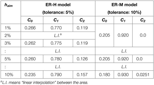
Table 6. Recommendation Values for C₀, C₁, and C₂ for the Extended Rayleigh damping model.

Confirmation Using Multiple Mass System Model

To test the proposed model in a time history response analysis, the case of 1 ~ 100 Hz, assuming f_lim = 100 Hz, was investigated.

Figure 14 shows the analysis model, and Table 7 gives its properties. One hundred single degree of vibration models were installed on a rigid beam, which was connected to the fixed end of a rigid spring. The masses were adjusted so that the value for each undamped resonant frequency was 1, 2, 3, …, 100 Hz. A time history response analysis was conducted by providing a unit pulse wave as the ground motion acceleration. The Newmark-β method (β = 1/4) was employed for the time integral. The analysis time step ΔT was set at 0.0005 s to allow the response in the high-frequency area to also be evaluated.

FIGURE 14

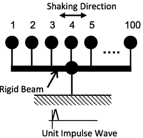
Figure 14. Multi-DOF model.

TABLE 7

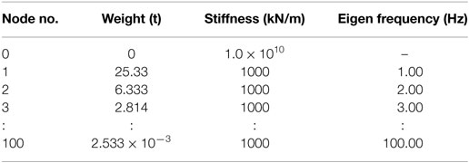
Table 7. Properties of the multi-DOF model.

The transfer function was calculated by dividing the response acceleration of each point by the ground motion acceleration in the frequency area, to examine the peak height of each transfer function. It is known that the theoretical value p with regards to the peak height of the transfer function for a one degree of freedom (DOF) system can be expressed by Eq. 34 as a function of the damping ratio h. Based on this, the obtained damping ratio h(ω₀) was calculated using Eq. 35 as a function of the peak height of each single DOF model p(ω₀), where ω₀ is the undamped resonant circular frequency. By comparing the result of this equation with the target damping ratio h_aim, the accuracy of the damping ratio R_h(ω₀) could be calculated.

$p=\frac{\sqrt{1+4h^2}}{2h}$ (34)

$h\left({\mathrm{\omega }}_0\right)=\frac{1}{2\sqrt{p{\left({\mathrm{\omega }}_0\right)}^2-1}}$ (35)

The theoretical value of the resonant circular frequency of the vibration system with damping ${\mathrm{\omega }}_0^{\prime }$ is given by Eq. 7 as the function of the undamped system resonant circular frequency ω₀. The accuracy of the resonant frequency realized for each model R_res(ω₀) could then be calculated by comparing the circular frequency corresponding to the peak value of each vibration system computed in the response analysis with this theoretical value.

Figure 15 shows the results from the analyses carried out using the Rayleigh damping model. The values for h_aim were set at 3 and 10% for ω₁ and 10 and 25.5 Hz for ω₂. This corresponds to the case with 10% tolerance shown in Table 1. White and black circles show the theoretical values at h_aim = 3 and 10%, respectively. These values were calculated for R_h(ω) using Eq. 5 and for R_res(ω) using Eq. 7. The results calculated by the response analyses are shown in the figure as solid and dotted lines. These calculated results corresponded well to the theoretical values. The validity of the analyses in this section was confirmed. R_h(ω) did not depend on h_aim, and there was a large difference between R_h(ω) and h_aim in most of the frequency area, with the exception of ω₁ and ω₂. As a result, R_res(ω) was consistent with Table 2.

FIGURE 15

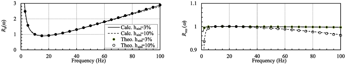
Figure 15. Damping ratio and damping frequency ratio (Rayleigh).

Figure 16 shows the results of the analysis of the causal model improved using Eq. 28. h_aim were set at 3 and 10%. R_h(ω) corresponded to Figure 11 and R_res(ω) to the C9 model shown in Figure 9. The results for R_h(ω) and R_res(ω) were equivalent to Figures 9 and 11, respectively.

FIGURE 16

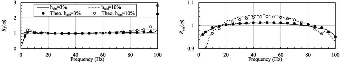
Figure 16. Damping ratio and damping frequency ratio (C9).

Figures 17 and 18 show the results of the high accuracy model (ER-H) and the middle accuracy model (ER-M) with h_aim at 3 and 10%. In ER-H, all values of R_h(ω) were within 0.95 ~ 1.05 in the area from 6 Hz to ~80 Hz, a tolerance within 5%. In ER-M, all the values of R_h(ω) were within 0.90 ~ 1.10 from 4 Hz to the vicinity of 85 Hz, giving a tolerance within 10%. The values of R_res(ω) in these figures correspond well to those of the C2 model shown in Figure 9.

FIGURE 17

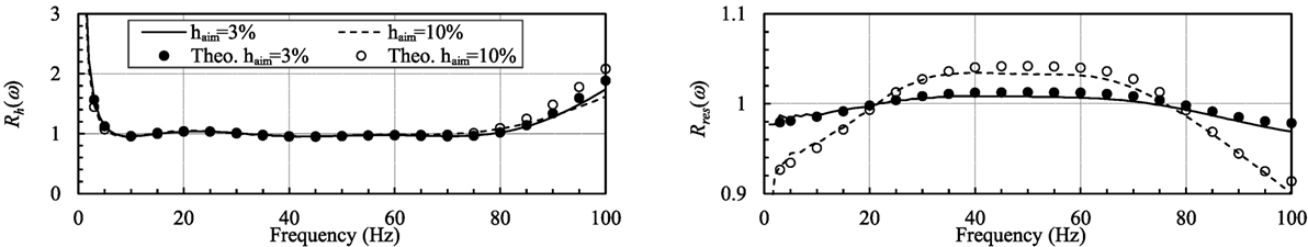
Figure 17. Damping ratio and damping frequency ratio (ER-H).

FIGURE 18

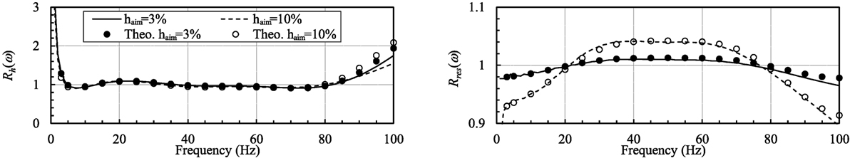
Figure 18. Damping ratio and damping frequency ratio (ER-M).

Table 8 shows the constant frequency area confirmed in these analyses. The value of W_h from the ER-H model was greater than 13.0. This is 5.3 ~ 5.5 times larger than the value from the Rayleigh model with the same tolerance. In the case where h_aim = 3% and f_lim = 100 Hz, for example, the frequency area from 6 ~ 82 Hz was within the tolerance. In the ER-M model, the values of W_h were greater than 21.3, or 5.6 ~ 5.8 times those of the Rayleigh model with the same tolerance. Using the same h_aim and f_lim, the constant frequency area was 4 ~ 85 Hz.

TABLE 8

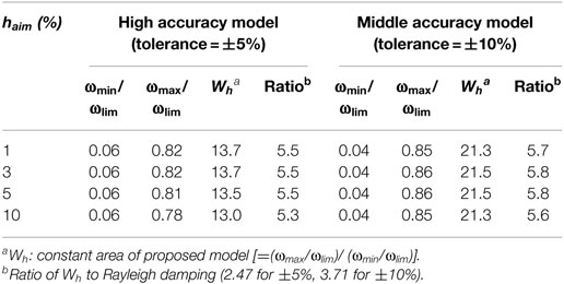
Table 8. Comparison of constant area with Rayleigh damping and the proposed model.

This demonstrates that the accuracy of the proposed model is higher than that of the Rayleigh model.

Example Analysis

To confirm the applicability of the proposed model to a practical structure, investigations were carried out using a 3-dimensional finite element model (hereafter referred to as 3D FEM).

Investigations Using a 3D FEM Model

To confirm the effectiveness of the proposed model as a practical multiple DOF model, investigations using a 3D FEM model were carried out. The analysis model was a dome-shaped structure with a diameter of 44 m, a height of 58 m, and a weight of 1400 t, as shown in Figure 19. The model was divided into 672 elements using shell elements, with 32 divisions in the circumferential direction. In the vertical direction, there were 10 divisions in the cylindrical part and 5 divisions in a dome part. The lowest points of the cylindrical part were fixed. Table 9 shows the principal properties of the model. Table 10 shows the principal natural frequency obtained from real eigenfrequencies, and the eigenmodes are given in Figure 20.

FIGURE 19

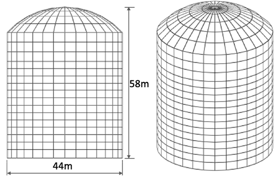
Figure 19. Analysis model.

TABLE 9

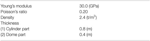
Table 9. Properties of the analysis model.

TABLE 10

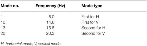
Table 10. Principal eigenfrequencies.

FIGURE 20

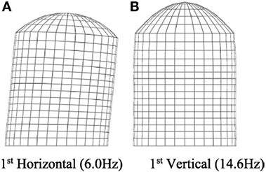
Figure 20. Principal Eigen Mode. (A) First horizontal (6.0 Hz) (B) First vertical (14.6 Hz).

The conditions for the time history response analysis were the same as those in the previous section. The time step ΔT was set at 0.0005 s to estimate the high frequency. The response acceleration at the nodal point of the top was obtained by providing a unit impulse in the horizontal direction as ground motion acceleration.

Transfer functions were calculated by dividing this response acceleration by the ground motion acceleration in the frequency area. Values of 3 and 10% were used for the damping ratio h_aim of the materials. The transfer functions were horizontal response outputs for horizontal direction inputs.

A frequency domain analysis (FDA) was carried out. This was assumed to give the correct answer to the problem, and the results were compared with those from the proposed model. Constant damping ratios of 3 and 10% were provided by the complex damping. The analysis pitch Δf in the frequency area was set to 0.1 Hz.

Figure 21 shows the results from the Rayleigh model, in which Case 1 and Case 2 (corresponding to Rayleigh-1 and -2) were investigated. In Case 1, a horizontal first-order frequency of 6 Hz was set for ω₁, and a vertical first-order frequency of 14.6 Hz was set for ω₂. In Case 2, the horizontal first-order frequency was set for ω₁, and ω₂ was set to 10 times ω₁. The results for Case 1 were very close to the FDA results in the area from 0 to nearly 20 Hz. However, in the area of 20 Hz and above, a large difference from the FDA emerged due to excessive damping. In Case 2, the results corresponded closely to FDA in the range 40 ~ 80 Hz because the ω₂ of this model was 60 Hz. However, a large difference in the peak values at the horizontal second-order frequency was seen in the vicinity of 15 Hz. These results confirmed that it is difficult for the Rayleigh model to express a constant damping ratio across a wide frequency area.

FIGURE 21

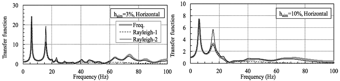
Figure 21. Transfer function [frequency response (FDA) vs. Rayleigh damping].

Figure 22 shows the results obtained using the C9 model described in Section “Improvement of the Causal Model.” The value for f_lim was set at 100 Hz. For the time delay part, nine terms for the displacement at 0.01, 0.02, 0.03, …, 0.09 s before the current time were considered. This model closely matched the response results of FDA in the area from 0 to almost 90 Hz when h_aim = 3%, and the area from 0 to almost 80 Hz when h_aim = 10%. However, when h_aim = 10%, a difference in the peak height of the horizontal first-order mode in the vicinity of 6 Hz was seen. This was caused by the reduction in the damping accuracy at both ends of the constant frequency area. It occurred when the damping ratio was large in the C9 model (cf., the results from C9 in Figure 11).

FIGURE 22

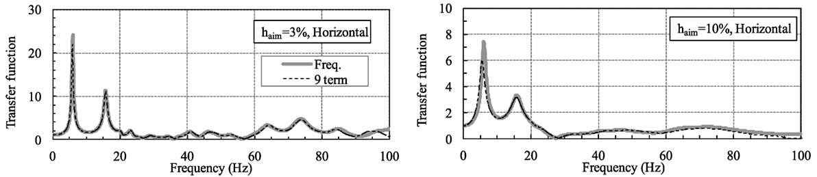
Figure 22. Transfer function [frequency response (FDA) vs. causal 9 term (C9)].

Figures 23 and 24 give the results from the ER-H and ER-M models. The f_lim value for ER-H was set at 100 Hz, and the displacement at 0.01 and 0.02 s before the current time were used in the time delay term. The f_lim value for ER-M was set at 150 Hz, and displacements at 0.0067 and 0.0133 s were used.

FIGURE 23

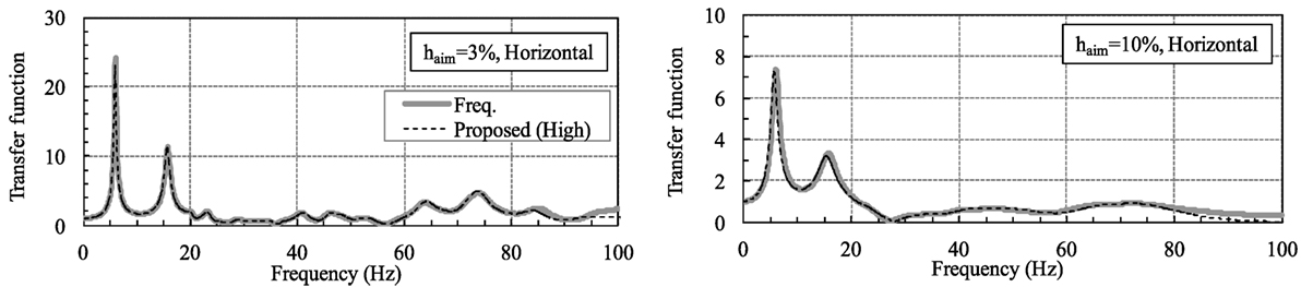
Figure 23. Transfer function [frequency response (FDA) vs. proposed high accuracy (ER-H)].

FIGURE 24

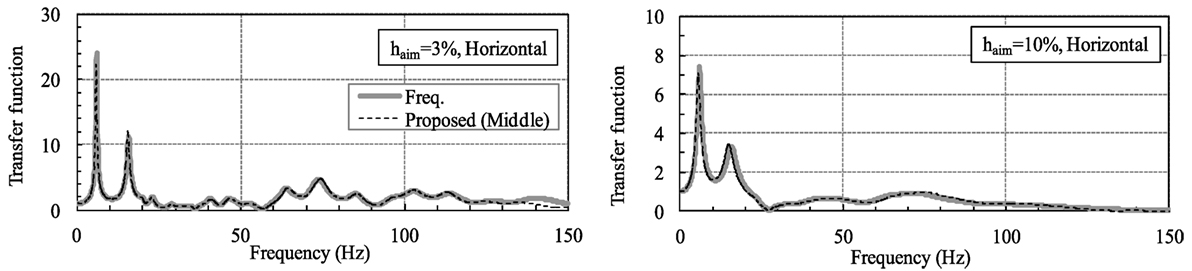
Figure 24. Transfer function [frequency response (FDA) vs. proposed middle accuracy (ER-M)].

The results from ER-H corresponded quite closely to those from the FDA in the area from 0 to almost 80 Hz. Although the accuracy of ER-M was slightly lower than that of ER-H in deriving the height of the peak value, the results from ER-M corresponded well in general to the results from the FDA in the area from 0 to almost 130 Hz. This confirmed the accuracy of the proposed models.

Conclusion

When time history response analysis is carried out using FEM, a Rayleigh damping model is often employed to take account of the constant damping characteristics for the frequency. However, the accuracy of this model is unsatisfactory. In this paper, we proposed a new model in which the stiffness proportional damping term of the Rayleigh model was replaced by that of the causal damping model. In this approach, the term of the coefficient sum for the past two time displacements is added to the standard Rayleigh model. This greatly improved the accuracy of the Rayleigh model. The effectiveness of the new models was confirmed by carrying out a trial analysis.

Future studies will be conducted to investigate the applicability of the new model to a range of model types and to large-scale models, especially those with tens of thousands of elements. We will also investigate its applicability to the element Rayleigh damping model, which is used when a total model has multiple damping ratios. In this study, the investigations were conducted on a linear level. Further studies are needed on the applicability of the model when elements become non-linear and the value of h_aim increases.

Author Contributions

The author confirms being the sole contributor of this work and approved it for publication.

Conflict of Interest Statement

The author declares that the research was conducted in the absence of any commercial or financial relationships that could be construed as a potential conflict of interest.

Funding

This work was supported by JSPS KAKENHI Grant Number 26289197.

References

Biot, M. A. (1958). “Linear thermodynamics and the mechanics of solids,” in Proc. 3rd U.S. National Congress of Applied Mechanics (ASME) Vol. 6 (Providence: R. M. Haythornthwaite), 1–18.

Google Scholar

Charney, F. A. (2008). Unintended consequence of modeling damping in structures. J. Struct. Eng. (N Y N Y) 134, 581–592. doi: 10.1061/(ASCE)0733-9445(2008)134:4(581)

CrossRef Full Text | Google Scholar

Chopra, A. K. (2001). Dynamics of Structures, 2nd Edn. NJ, USA: Prentice-Hall.

Google Scholar

Chouw, N. (2002). Influence of soil-structure interaction on pounding response of adjacent buildings due to near-source earthquake. J. Appl. Mech. 5, 543–553. doi:10.2208/journalam.5.543

CrossRef Full Text | Google Scholar

Erduran, E. (2012). Evaluation of Rayleigh damping and it influence on engineering demand parameter estimates. Earthq. Eng. Struct. Dyn. 41, 1905–1919. doi:10.1002/eqe.2164

CrossRef Full Text | Google Scholar

Hall, J. F. (2006). Problems encountered from the use (or misuse) of Rayleigh damping. Earthq. Eng. Struct. Dyn. 35, 525–545. doi:10.1002/eqe.541

CrossRef Full Text | Google Scholar

Inaudi, J. A., and Kelly, J. M. (1995). Linear hysteretic damping and the Hilbert transform. J. Eng. Mech. 121, 626–632. doi:10.1061/(ASCE)0733-9399(1995)121:5(626)

CrossRef Full Text | Google Scholar

Jehel, P., Legar, P., and Ibrahimbegovic, A. (2013). Initial versus stiffness-based Rayleigh damping in elastic time history seismic analysis. Earthq. Eng. Struct. Dyn. 43, 467–484. doi:10.1002/eqe.2357

CrossRef Full Text | Google Scholar

Makris, N. (1997). Causal hysteretic element. J. Eng. Mech. 12, 1209–1214. doi:10.1061/(ASCE)0733-9399(1997)123:11(1209)

CrossRef Full Text | Google Scholar

Makris, N., and Zhang, J. (2000). Time domain viscoelastic analysis of earth structures. Earthq. Eng. Struct. Dyn. 29, 745–768. doi:10.1002/(SICI)1096-9845(200006)29:6<745::AID-EQE937>3.0.CO;2-E

CrossRef Full Text | Google Scholar

Muscolino, G., Palmeri, A., and Ricciardelli, F. (2005). Time-domain response of linear hysteretic systems to deterministic and random excitations. Earthq. Eng. Struct. Dyn. 34, 1129–1147. doi:10.1002/eqe.471

CrossRef Full Text | Google Scholar

Nakamura, N. (2006). A practical method to transform frequency dependent impedance to time domain. Earthq. Eng. Struct. Dyn. 35, 217–231. doi:10.1002/eqe.520

CrossRef Full Text | Google Scholar

Nakamura, N. (2007). Practical causal hysteretic damping. Earthq. Eng. Struct. Dyn. 36, 597–617. doi:10.1002/eqe.644

CrossRef Full Text | Google Scholar

Nakamura, N. (2008). Transform methods for frequency dependent complex stiffness to time domain using real or imaginary data only. Earthq. Eng. Struct. Dyn. 37, 495–515. doi:10.1002/eqe.767

CrossRef Full Text | Google Scholar

Nakamura, N. (2012). A basic study on the transform method of frequency dependent functions into time domain-relation to Duhamel’s integral and time domain transfer function. J. Eng. Mech. 138.3, 276–285. doi:10.1061/(ASCE)EM.1943-7889.0000330

CrossRef Full Text | Google Scholar

Nakamura, S., Nakamura, N., Suzuki, T., Inoda, K., and Kosaka, K. (2012). “Study on the influence of irregular ground and adjacent building on the seismic response of nuclear power plant building,” in Proc. 15 the World Conference of Earthquake Engineering, Lisboan, Portugal, Paper No. 1086.

Google Scholar

Onimaru, S., Hamada, J., Nakamura, N., and Yamashita, K. (2012). “Dynamic soil-structure interaction of a building supported by piled raft and ground improvement during the 2011 Tohoku earthquake,” in Proc. 15 the World Conference of Earthquake Engineering, Lisboan, Portugal, Paper No. 3681.

Google Scholar

Ryan, K. L., and Polanco, J. (2008). Problems with Rayleigh damping in base-isolated building. J. Struct. Eng. 134, 1780–1784. doi:10.1061/(ASCE)0733-9445(2008)134:11(1780)

CrossRef Full Text | Google Scholar

Spanos, P. D., and Tsavachidis, S. (2001). Deterministic and stochastic analyses of a nonlinear system with a biot visco-elastic element. Earthq. Eng. Struct. Dyn. 30, 595–612. doi:10.1002/eqe.29

CrossRef Full Text | Google Scholar

Zareian, F., and Medina, R. A. (2010). A practical method for proper modeling of structural damping in inelastic plane structural systems. Comput. Struct. 88, 45–53. doi:10.1016/j.compstruc.2009.08.001

CrossRef Full Text | Google Scholar