Structural Identification of an 18-Story RC Building in Nepal Using Post-Earthquake Ambient Vibration and Lidar Data

Introduction

This paper presents data collection, structural identification, and finite element (FE) modeling of an 18-story reinforced concrete (RC) building in Kathmandu that was damaged during the Gorkha earthquake. The Gorkha earthquake, with a moment magnitude of 7.8, struck Nepal on April 25, 2015. Several strong aftershocks followed the main shock, including a magnitude 7.3 aftershock that occurred on May 12, 2015, 17 days after the main shock (Rai et al., 2015). More than 8,000 people died, and nearly half a million buildings were damaged. The capital of Nepal, Kathmandu, has a high population density and is highly urbanized. It is also one of the worst affected regions, likely due to the basin effects of the Kathmandu valley. Information on the performance of structures during the 2015 Gorkha Earthquake can be found in Brando et al. (2015).

In this study, post-earthquake ambient response of the building is collected using a course array of accelerometers. For structural identification, modal parameters (natural frequencies, damping ratios, and mode shapes) of the building are estimated using an operational modal analysis (OMA) approach from ambient acceleration response of the building collected at selected floors. The Natural Excitation Technique (James et al., 1992) combined with the Eigensystem Realization Algorithm (Juang and Pappa, 1985) (NExT-ERA) is used for system identification. Experimental modal analysis methods extract modal parameters of a structural system based on measurements of both the dynamic response and the input excitation. On the other hand, output-only or OMA methods are used when the ambient response of a structure is the only measurement with the input excitation unknown and/or unmeasured. These system identification methods provide accurate results when the unmeasured input excitation can be assumed as a broadband random signal such as wind loads on a building or vehicular traffic on a bridge and are often used for large-scale civil structures, which are difficult to excite experimentally (Brincker and Kirkegaard, 2010). Several OMA methods have been introduced in the literature and can be classified into two groups based on the type of data they use: frequency-domain methods and time-domain methods (Peeters and De Roeck, 2001). Among the frequency domain methods, peak-picking method is the most common approach for estimating the modal parameters. However, the accuracy of estimated modal parameter degrades when the vibration modes are closely spaces and/or highly damped. To address this shortcoming, Brincker et al. (2001) proposed the frequency domain decomposition method where peak-picking is enhanced with singular value decomposition. More recently, a probabilistic version of frequency domain decomposition method is proposed by Au et al. (2013), which allow estimating the probability density function of modal parameters instead of a single estimate. Building on this, a two-stage Bayesian system identification has been developed to determine the structural parameters such as mass and stiffness from ambient vibration data (Au and Zhang, 2016; Zhang and Au, 2016).

One of the most commonly used time-domain system identification methods includes the NExT-ERA method, also known as covariance-driven stochastic subspace identification (SSI), which is used in this study, as well as the data-driven SSI method (Van Overschee and de Moore, 1996). These methods have been successfully applied for system identification of large-scale civil structures. In an earlier study, Feng et al. (1998) successfully identified the modal parameters of the Nanjing TV Tower using sparsely measured ambient acceleration response. Brownjohn (2003) applied the NExT-ERA and peak-picking methods for OMA of two tall buildings. Antonacci et al. (2012) evaluated the performance of four output-only modal identification methods using experimental data extracted from the ambient vibration response of a three-dimensional frame. Cunha et al. (2013) reviewed dynamic testing and system identification of four case study bridges in Europe. Moaveni et al. (2014) compared the performance of three OMA methods (SSI, NExT-ERA, and frequency domain decomposition) for system identification of a seven-story shear wall structure using experimental and numerical data. Belleri et al. (2014) estimated the modal parameters of a three-story precast concrete parking structure at different damage states and identified the location of damage from the changes in modal parameters.

In addition to the vibration measurements, a total of 16 lidar scans from the building’s interior were collected at selected floors. Then, a damage detection algorithm uses these lidar-derived point clouds to explore the damage evolution for two common members based on the agreement of two distinct methods that evaluate surface geometry. Previous researchers have used the lidar-derived point clouds for structural assessment and detecting damage. Examples include Kim et al. (2014) and Guldur and Hajjar (2014) who investigated the variations of the surface normals to detect damaged regions of a member. Kim et al. (2014) used Principal Component Analysis (PCA) of each vertex and its eight nearest neighboring vertices to estimate surface normals and then compared each surface normal to a normal vector of the plane fitted to the entire data set. This proposed workflow could successfully detect the damaged areas; however, the method is limited to detection of shallow defects in small-sized planar surfaces. Similarly, Guldur and Hajjar (2014) performed the damage detection of point clouds by using various methods including the variation of surface normals. Although, this method can detect defects, construction of the reference vectors requires numerous lengthy processes (segmentation, curvature computation, and identifying the member geometry). In the study discussed here, a damage detection algorithm is developed to detect and quantify the surface defect percentage from both singular and multi-planar surfaces through direct computation of surface normals and comparing them to a corresponding local reference vector and estimating the surface variation of each vertex with respect to its nearest vertices.

Finally, a linear FE model of the building is developed using the available geometry and material properties. Dynamic properties of the model are compared to those obtained from system identification. The validated model is then used to predict the response of the structure when subjected to the Gorkha earthquake and one of the main aftershocks. The predicted inter-story drift ratios are compared with level of observed damage and lidar data at different stories along the height of the building.

Test Structure and Collected Data

The structure considered in this study, also referred to as the CityScape #1 building, is an 18-story (basement plus 17 stories above ground) RC building located in Hattiban, Katmandu, Nepal. The building is shown in Figure 1A, while a typical floor plan is shown in Figure 1B. The building was designed for shaking intensities larger than those experienced in this seismic sequence [IS 13920, 1993; IS 1893 (part 1), 2002]; hence, it maintained life-safety despite the extensive damage, mainly in non-structural elements such as masonry walls. These walls in some cases were infills within RC frames, while in other cases they were only connected to the slabs above and below without being confined by beams and columns. As a result they separated from the RC members and developed extensive cracks in a number of stories. Moderate non-structural and slight structural damage was also observed as beam-column joint cracks, and shear cracks were visible in coupling beams and short beams. Additionally, flexural cracks on beams propagated to the 125-mm thick slabs at a few locations.

FIGURE 1

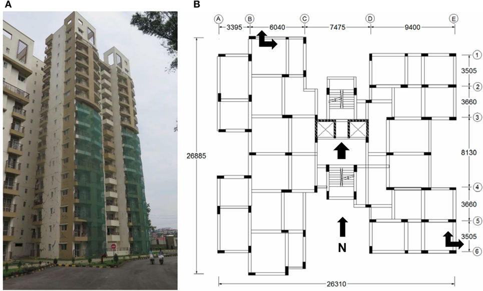
Figure 1. Building details and instrumentation setup. (A) Front view of Cityscape #1 building. (B) Typical floor plan (units in millimeter).

The observed damage is repairable, although the repair cost can be very high. Figure 2 shows examples of the observed damage on different components of the building including (a) non-structural damage in exterior walls, (b) beam-column joint cracking, (c) non-structural damage in interior infill walls, and (d) separation between column and infill. The visual inspection together with surface defect detection (from the lidar data) provides a basis for stiffness reduction of section properties discussed in the FE modeling section.

FIGURE 2

Figure 2. Observed damage on different components of the building. (A) Exterior damage. (B) Beam-column joint. (C) Interior infill wall. (D) Separation between column and infill.

Vibration Measurements

The ambient vibration response of the building was measured using 15 uniaxial accelerometers that were installed in two distinct configurations due to the number of stories, the length of cables, and the number of available sensors. In the first setup (Setup 1), accelerometers were installed on floors 9, 12, and 15; while in the second setup (Setup 2), floors 3, 6, and 9 were instrumented. Table 1 reports the location and direction of the eight available accelerometers in each setup. The data measured by each setup includes approximately 1 h of ambient vibration recordings. On each instrumented floor, five or six accelerometers were installed in the center, as well as in the north-west (NW) and south-east (SE) corners of the building. Figure 3A shows the location of sensors at each floor and along the height of building. The arrows on Figure 1B also indicate the location and direction of accelerometers. The location of sensors was selected such that the torsional motion of the building can be captured. The accelerometers were mounted on brackets, which were then attached to the floors using double-sided tape. The sensors were wired to a National Instruments compact DAQ through BNC cables, and the data were saved locally on a laptop. Figure 4 shows the used compact DAQ and an in situ sensor installation.

TABLE 1

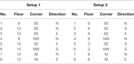
Table 1. Location and direction of sensors in first setup (Setup 1) and second setup (Setup 2) (SE, south-east; NW, north-west; M, middle).

FIGURE 3

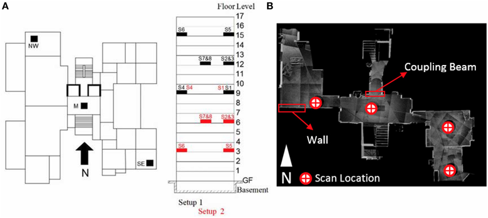
Figure 3. Sensor and lidar scans layout. (A) Elevation view with the distribution of the sensors for Setups 1 and 2. (B) Top view of typical scan placements per floor and locations of scanned members.

FIGURE 4

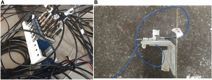
Figure 4. Data acquisition system and accelerometers installation. (A) Compact DAQ. (B) Sensor and bracket taped to floor.

Data from seven sensors were found too noisy; therefore, only eight are considered in the analysis. Low signal-to-noise ratio at these sensors could be due to the poor quality of BNC cables and/or their end connectors which were connected on site. It is worth noting that in general, it is not possible to completely characterize the dynamic properties of a complex tall building with eight uniaxial accelerometers. However, the performed system identification allows accurate estimation of natural frequencies and damping ratios of the dominant vibration modes as well as the mode shape estimates of the lower vibration modes with a course resolution. To calibrate the used sensors and evaluate the sensor mounting, a shaker test was carried out at Tufts University after the completion of in situ tests. The results show that (1) the calibration factors of sensors have not changed from their nominal values except for one sensor, which appears to be damaged in its return transit to the US, and (2) the mounting tape does not affect the recorded signal properties in the frequency range of interest. More details about the shaker tests can be found in Yu (2016).

Lidar Data Collection

To perform a reconnaissance survey of the damage, the team used a Faro Focus X-130 lidar scanner. This scanner can capture up to nearly one million points per second with an effective range of 130 m and a tabulated error of ±2 mm (FARO, 2011). The team performed a total of 16 scans from the building’s interior on the third, sixth, ninth, twelfth, and fifteenth floors (same as the ambient vibration floor levels) to document the variation of damage the building sustained. As anticipated, the level of damage to structural and non-structural components at lower floors was notably higher than to those of upper levels due to their drift sensitivity. Figure 3B illustrates the typical scanner location for each floor where a total of four scans were conducted per floor level. In addition, the location for the common members, the coupling beam, and an example wall are highlighted in Figure 3B for the third floor.

Surface Defect Detection from Lidar Point Clouds

To investigate and quantify the damage pattern as a function of story level, a portion of the point cloud is extracted for a single beam at the selected levels and analyzed using a damage detection algorithm as shown in Figure 5A. The selected member is a coupling beam, which contains dual planar surfaces which sustained notable varying damage at select levels. In addition, point cloud of a common wall, a singular or flat planar surface where the FE model results predicts large damage, is explored for damage detection and quantification (Figure 5B).

FIGURE 5

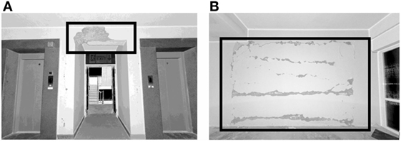
Figure 5. The members selected to investigate the damage evolution. (A) Coupling beam. (B) Infill wall.

To detect damage and quantify surface defect percentage of the extracted point clouds, the algorithm investigates the variation of surface normal and variations of each vertex with respect to local reference vector and nearest neighboring vertices, respectively. The algorithm initiates the analysis by performing a down-sampling process based on a voxel-grid filter with a point-to-point spacing, set equal to 0.5 cm in this case. Then, the algorithm directly computes the surface normals using a weighted-average method for n nearest neighbors (Jin et al., 2005). Once the surface normals are computed, the reference vector for each vertex is calculated using a least square plane over n′ nearest neighbors (Shakarji, 1998). These two vectors are compared in terms of a relative angle for each vertex via a dot product. To find the surface variation, initially the PCA is performed for each vertex and its selected nearest vertices to find the eigenvalues of the covariance matrix corresponding to each vertex and its nearest vertices. Then, the surface variation of each vertex is calculated through computing the ratio of smallest eigenvalue with respect to the summation of all eigenvalues (Pauly et al., 2002). Within this study, the neighboring sizes of 8, 8, and 24 were found via a kd-tree search algorithm and used for the computation of surface normal, surface variation, and the local reference planes, respectively. To locate and identify potential defects, the probability distribution for change in surface variation and the relative angle are constructed based on Kernel distributions. The Kernel distributions were selected due to its minimal assumptions of the underlying distribution. In the final step, a damage verification algorithm classifies a vertex as possible damage if and only if its relative angle and surface variation values are located at the 45 and 60% threshold of their respective kernel distributions for coupling beams and walls, respectively.

Table 2 presents the summarized values for surface defect percentages, and the detected surface defects are shown in Figures 6 and 7 for walls and coupling beams, respectively. It should be noted that the defect percentages are not directly correlated with loss of stiffness or strength but they provide qualitative measures of the structural damage at the surface. The detected defects and sharp edges are shown by red color (gray in black and white prints), while the undamaged areas are shown by black color. As illustrated by Figure 6, the third, ninth, and twelfth floor walls exhibited moderate cracking and localized spalling with identified surface defect percentages of 15, 12, and 7%, respectively (Figures 6A,B,E,F,H,I). The sixth floor wall exhibited moderate to extensive shear and horizontal cracking and moderate-depth spalling at the center of the wall (Figures 6C,D) with a surface defect percentage of 32%. As for the coupling beam, the member sustained significant damage at third and sixth stories with surface defect percentage of 50 and 47%, respectively (Table 2). However, this percent was reduced at higher stories, as it was found to be 30, 15, and 9% for the ninth, twelfth, and fifteenth floors, respectively. Figure 7 demonstrates the identified surface defects for coupling beams at third, sixth, and ninth floors. Additionally, the third floor coupling beam sustained significant spalling of its concrete cover in the middle with minor spalling at its two bottom end where the beam connects to the walls. This damage can be classified as moderate (Figures 7A,B). Despite the surface defect percentage for the coupling beam at the sixth story is reduced in comparison to the third floor’s beam, its damage is more severe (Figures 7C,D). This coupling beam exhibited significant localized concrete cover spalling with exposed reinforcement. The ninth floor beam, shown in Figures 7E,F, exhibited only modest concrete cover spalling at its midspan, likely only due to flexural loads. The results of surface defects for the two members considered here indicate that the structure sustained more damage at the mid-elevations, likely due to the contribution of higher modes, where only moderate to small damage was quantified at lower and higher stories. This is consistent with the maximum inter-story drifts during the earthquake estimated by the FE model.

TABLE 2

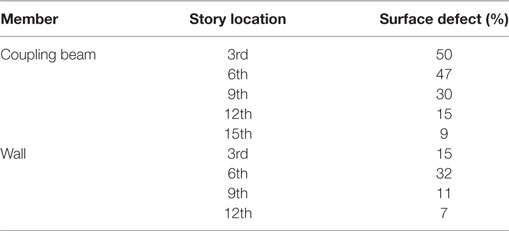
Table 2. Surface defect percentage values of selected members at various levels.

FIGURE 6

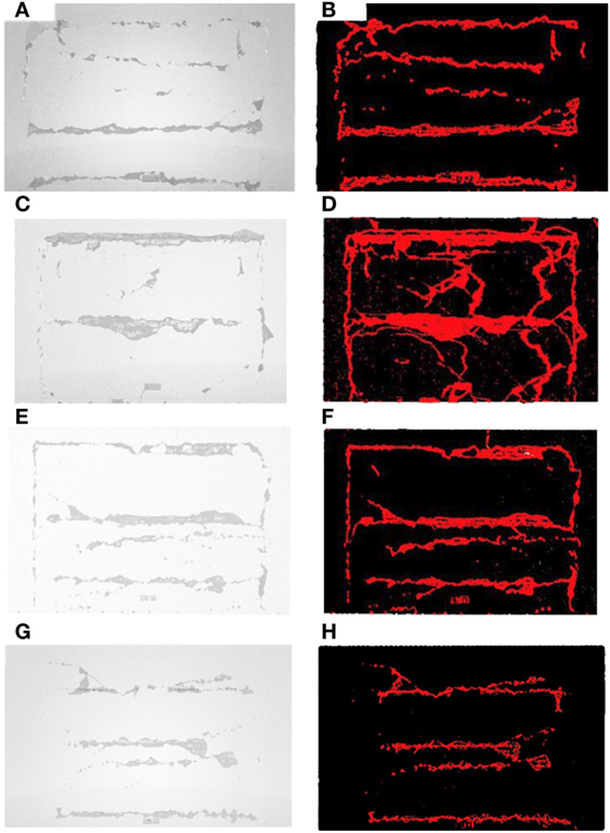
Figure 6. Evidence of damage at select floors for the common wall. (A) Third story black and white point cloud, (B) third story color-coded point cloud, (C) sixth story black and white point cloud, (D) sixth story color-coded point cloud, (E) ninth story black and white point cloud, (F) ninth story color-coded point cloud, (G) 12th story black and white point cloud, and (H) 12th story color-coded point cloud.

FIGURE 7

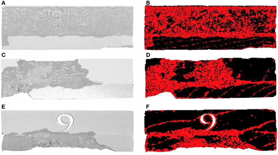
Figure 7. Illustration of damage propagation in the common coupling beam. (A) third story black and white point cloud, (B) third story color-coded point cloud, (C) sixth story black and white point cloud, (D) sixth story color-coded point cloud, (E) ninth story black and white point cloud, and (F) ninth story color-coded point cloud.

System Identification

Data Processing

The recorded ambient response data are used for estimating the modal parameters of the building using the NExT-ERA method. This method has been previously applied successfully for OMA of civil structures (Caicedo et al., 2004; He et al., 2006; Siringoringo and Fujino, 2008; Brownjohn et al., 2010; Sim et al., 2010; Moaveni et al., 2014). The obtained raw data are first processed to mitigate signal noise and remove voltage spikes. The processing procedure includes

(1) Filtering: data are filtered by applying a band-pass Finite Impulse Response (FIR) (Digital Signal Processing Committee of the IEEE, 1979) filter. In the initial analysis, the frequency range is chosen to be 0.2–10 Hz.

(2) Down-sampling: the filtered data is down sampled from 2,048 to 256 Hz to improve the computational efficiency with no adverse effect on resolution of system identification results.

(3) Spike removal: observed voltage spikes are manually removed (set to zero) in the measured acceleration time history signals.

According to the available data length in each setup, the recorded ambient vibration data is divided into six segments (referred herein as datasets). Each dataset corresponds to a 9-min long ambient vibration recording except for the last dataset of Setup 1, which is approximately 6-min long. Figure 8 presents the Fourier Amplitude Spectral (FAS) of the dataset 2 in Setup 1 for all eight channels. In this plot, peaks corresponding to the vibration modes of the building can be observed.

FIGURE 8

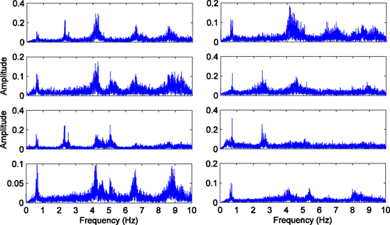
Figure 8. Fourier Amplitude Spectral of dataset 2 in Setup 1.

In the application of NExT, the cross power spectral densities (CPSD) are calculated between all eight channels and two reference channels using eight Hamming windows with a 50% overlap. The reference channels are chosen such that their power spectral densities provide clear peaks at the vibration modes of interest. The free vibration response of the building is then estimated as the inverse Fourier transformation of CPSD. The ERA method is used to identify the modal parameters from these free vibration estimates. To apply ERA, 800 data points or 3.125 s of derived free vibration data are used to form a 3,200 × 800 Hankel matrix, and a state-space model is realized through singular value decomposition of the Hankel matrix. The order of state-space model is determined using stabilization diagrams (Verboven et al., 2002). Figure 9 shows a sample stabilization diagram of natural frequencies. In this plot, the natural frequencies are plotted versus increasing model orders. The “stable” natural frequencies refer to the ones that are repeatedly identified and are shown with red lines in the plot. To avoid modeling redundancies, the model order should be chosen as the lowest order that can provide all of the mode of interest. Modal parameters of the building for each of the 12 datasets are estimated.

FIGURE 9

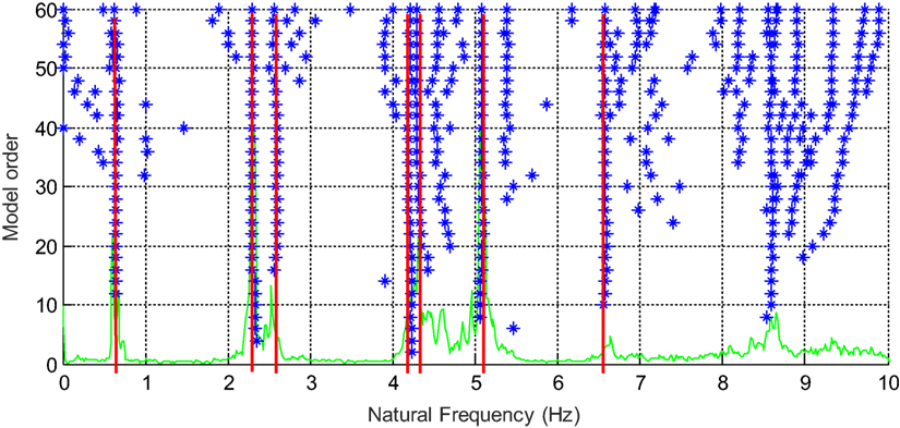
Figure 9. Sample stabilization diagram of natural frequencies.

Results of Modal Analysis Focused on 0.2–10 Hz

In Table 3, the statistics (mean and standard deviation) of identified natural frequencies and damping ratios are reported for each of the two setups over the six datasets. The small standard deviation (SD) of identified natural frequencies indicates their consistency across the six datasets in both setups. Comparison of the mean values of two setups demonstrates an excellent agreement with a maximum difference of 2.3% (mode 3). Thus, the natural frequencies are identified very consistently among the datasets and between setups. For damping ratio, larger SD is observed and consequently a less than ideal agreement is found between two setups. This is most likely due to larger estimation variance and bias for damping ratios compared to natural frequencies (Pintelon et al., 2007; Reynders et al., 2008). The damping estimate mean values are reasonable for a tall building except for that of mode 1 (Satake et al., 2003; Harris et al., 2015). The mean values of identified damping ratio for the first mode is 5.1% for Setup 1 and 7.5% for Setup 2, that are too large for a tall building (Arakawa and Yamamoto, 2004; Çelebi et al., 2014). This can be caused by the fact that three closely spaced modes with natural frequencies around 0.6 Hz are identified as one mode with an inflated damping ratio to account for the three peaks.

TABLE 3

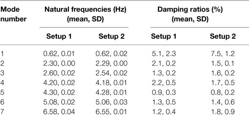
Table 3. Statistics of identified modal parameters in 0.2–10 Hz range.

Results of Modal Analysis Focused on 0.2–1 Hz

Based on the FE model of the building that is discussed later in Section “FE Modeling and Response Prediction,” the first three vibration modes of the building are very closely spaced at the frequency range of below 1 Hz. Such closely spaced modes could not be reliably identified in the previous application of OMA when looking at 0.2–10 Hz range due to the lower resolution of CPSD. Figure 10 shows the time history and FAS of channel 2 in dataset 1. From the FAS plot, three distinct peaks can be observed in the 0.55–0.75 Hz range. Therefore, in this section, modal analysis is carried out again focusing on the frequency range of 0.2–1.0 Hz. The procedure is similar to that of initial analysis, except a few differences in the data processing. A different FIR filter is used with the band-pass frequency range of 0.2–1.0 Hz. To ensure the sharpness of the filter edge and its smoothness within the band-pass range, the order of filter is selected as 65,536, which is 32 times the sampling frequency. Similar down-sampling and voltage spike removal steps are performed for the data cleaning process.

FIGURE 10

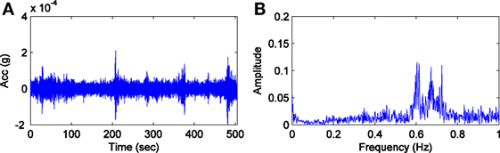
Figure 10. Sample measurement at channel 2 in dataset 1. (A) Time history. (B) Fourier Amplitude Spectrum.

In the application of NExT-ERA, the reference channels are chosen separately for the three modes of interest to ensure the identification of that mode. Since the first three vibration modes of the building are very closely spaced, a high frequency resolution is required for the CPSD estimates. Therefore, either three or five Hamming windows with 50% overlap are used resulting in frequency resolution of 0.005 or 0.007 Hz. The choice of three or five windows for each data set is made based on the stability and consistency of results. The order of the state-space model to fit the data is selected using stabilization diagrams for natural frequencies, as well as damping ratios and mode shapes. In these plots, the identified natural frequencies and associated damping ratios and Modal Assurance Criterion (MAC) values are plotted versus different model orders. MAC values quantify the similarity of two mode shapes. The MAC value between two mode shapes Φ₁ and Φ₂ is defined as (Allemang and Brown, 1982):

$\text{MAC}\left({\mathbf{\Phi }}_1,{\mathbf{\Phi }}_2\right)=\frac{{\left|{\mathbf{\Phi }}_1^{*}{\mathbf{\Phi }}_2\right|}^2}{\left|{\mathbf{\Phi }}_1^{*}{\mathbf{\Phi }}_1\right|\left|{\mathbf{\Phi }}_2^{*}{\mathbf{\Phi }}_2\right|}$ (1)

with superscript * denoting Hermitian transpose (or conjugate transpose). The MAC values can vary between 0 and 1, often expressed in percent. A MAC value of unity means that the two mode shapes are exactly the same, while a MAC of null indicates that the two mode shapes are perpendicular. Figure 11 shows sample stabilization diagrams for damping ratios and mode shapes. The three identified vibration modes are referred to as modes 1a, 1b, and 1c since they were collectively identified as mode 1 in the initial identification. Note that identification of mode 1a is performed separately from modes 1b and 1c due to different choices of reference channels. It can be observed that the damping ratios are stable for modes 1b and 1c but show some deviations at orders 32–36 for mode 1a. MAC values in the stabilization diagrams are computed between a selected order (which is deemed stable by the analyst) and all other model orders. The reference order for computation of MAC values in this study is 20. It is seen that the mode shapes are very consistent across different model orders, and thus, the identified mode shapes are robust with respect to the choice of model order in the identification process.

FIGURE 11

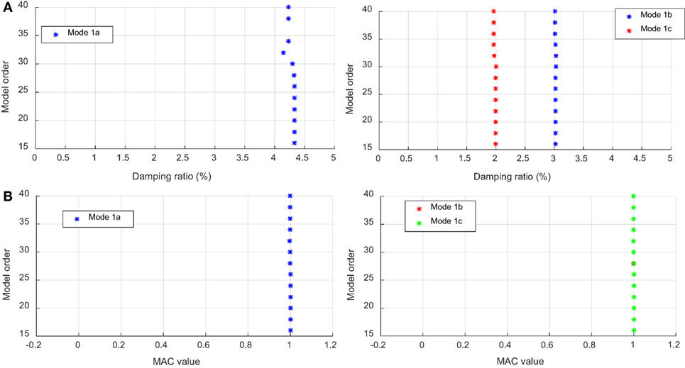
Figure 11. Sample stabilization diagram for damping ratios and mode shapes. (A) Stabilization diagram of damping ratios. (B) Stabilization diagram of mode shapes (MAC values).

The mean and SD of the identified natural frequencies and damping ratios over six datasets for Setups 1 and 2 are reported in Table 4. Similarly, the natural frequencies are identified consistently among datasets and between setups with a maximum difference 0.8% for mode 3. The damping ratios show larger variability across different datasets as indicated by the reported values of SD. The average damping ratios for the three modes and two setups vary between 1.3 and 2.8%, which are much more reasonable and anticipated for a tall RC building than the initial identification results.

TABLE 4

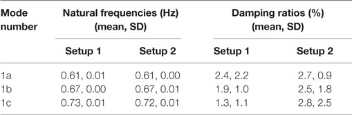
Table 4. Statistics of the identified natural frequencies and damping ratios in 0.2–1.0 Hz range.

These three mode shapes are also identified for each dataset and the two setups. An average mode shape is estimated for each setup based on the consistent mode shape estimates from the six datasets. To determine the “consistent mode shapes” to be used in the average, MAC values are computed pairwise between all datasets. The datasets with the MAC value lower than approximately 0.9 are considered inconsistent with other datasets and therefore are not considered in the averaging process. As an example, Table 5 shows the MAC values between different datasets for mode 1c. In this case, mode shapes from datasets 2 and 4 are considered inconsistent (underlined in the table), and therefore, only mode shapes of datasets 1, 3, 5, and 6 are used in averaging. Once the average mode shapes of Setups 1 and 2 are obtained, these mode shapes are combined to represent the complete mode shapes of building along its full height. The mode shapes from the two setups are combined by normalizing the mode shapes to one of the two channels that are available for both setups: Channel 1 (at SE corner of ninth floor measuring in north direction) and Channel 4 (at NW corner of ninth floor measuring in north direction).

TABLE 5

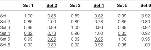
Table 5. Modal Assurance Criterion (MAC) values between mode shapes of mode 1c from different datasets.

Figure 12A presents the combined mode shapes using reference channel 4, while the complex-valued mode shapes are plotted in Figure 12B as compass plots. In Figure 12A, x-axis indicates the real value of mode shapes while y-axis indicates the floor. Solid lines show the identified mode shape, and dashed lines show mode shapes of the FE model. The blue lines (with square markers) correspond to motions at the NW corner of the building along the north-south direction and green lines (with triangle markers) correspond to motions at the SE corner of the building along the east-west direction. Also in this figure, the “*” indicates the position of reference channel used for normalization. From Figure 12A, it can be seen that the first two identified modes (1a and 1b) have torsional components, while the motion of the third identified mode (1c) is mainly in the north-south direction. The horizontal and vertical axes of the compass plots in Figure 12B correspond to the real and imaginary values of mode shape components. Each arrow in the plot represents a complex-valued mode shape component (i.e., at a sensor location). While the mode shapes of civil structures are often real-valued, the components of mode shapes in this plot are not completely aligned along the real axis indicating that the identified modes are to some degree non-proportional (i.e., not classically damped). The fact that the modes are identified as non-proportional indicates some identification errors that are most likely caused by the poor and uneven signal-to-noise ratios among different channels (sensors and cables).

FIGURE 12

Figure 12. Identified mode shapes from both setups. (A) Identified mode shapes along the height together with mode shapes of FE model. (B) Compass plots of identified mode shapes.

FE Modeling and Response Prediction

FE Model Properties

A linear FE model of the 18-story building is developed using the SAP2000 structural analysis software (Computers and Structures Inc., 2013) as shown in Figure 13. The basement is herein considered as pinned supports at its base (below the ground level) and with rollers applied perpendicular to the exterior basement walls at the ground level, constraining the lateral motion of the building at the ground level and neglecting any soil–structure interaction. All RC beams are assumed to have a 500 mm × 350 mm cross sectional dimensions, as obtained from the design drawings. Concrete slabs are 125 mm thick. For the RC elements (beams, columns, and shear walls), the mechanical properties used are based on a nominal compressive strength of 30 MPa and an expected strength of 33 MPa. This expected strength was determined based on Schmidt hammer testing performed on site. The average value of the concrete compressive strength estimated is 33 MPa based on measurements for three RC Beams with inter-test coefficient of variation of 0.21 between all tested locations. The expected compressive strength was used in assigning properties to the FE model.

FIGURE 13

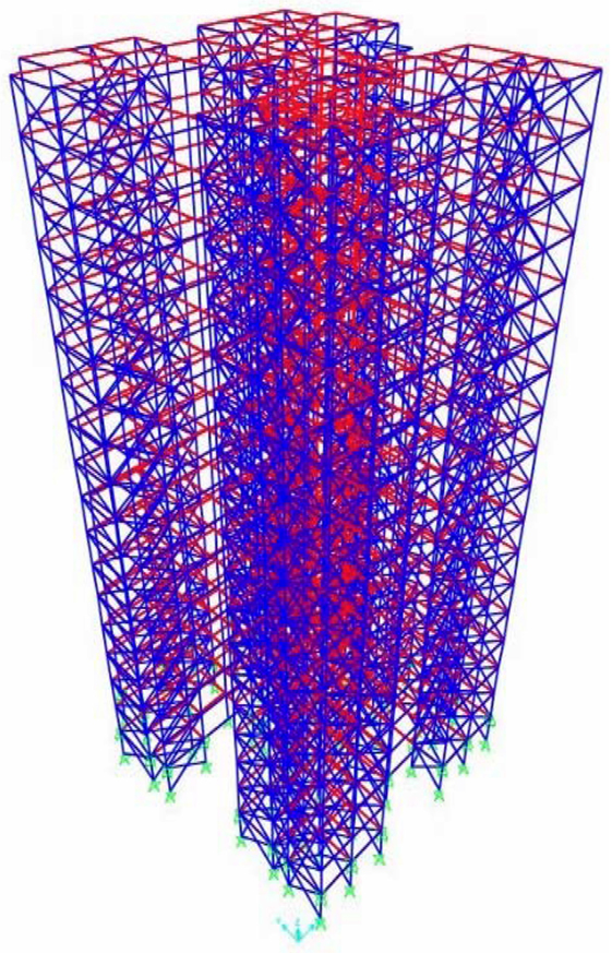
Figure 13. Finite element model of the building in SAP2000.

In the FE model, the shear walls are modeled using four-node shell elements. Three-dimensional linear frame elements are used to model all the beams and columns of the building. For modeling the infill walls, the equivalent diagonal strut method is used (Saneinejad and Hobbs, 1995). In this method, each infill wall panel was replaced with two diagonal compression-only struts. The guidelines in FEMA 356-2000 (Federal Emergency Management Agency, 2000), which are based on the work of Stafford Smith and Carter (1969) and Mainstone (1971), are used to determine the equivalent width of the struts. The tension limit and end moments of the frame element used to model the infill walls are set to 0 in order to model the diagonal compression-only struts. Values assumed for the masonry compressive strength and Young’s modulus are 4.5 and 2,400 MPa, respectively. Stiffness reduction factors are applied to account for panel openings depending on size of the opening, as per design drawings, ranging from 0.3 to 0.7. An additional stiffness reduction factor with different values is used to simulate the observed damage in the masonry infill walls of the building after the earthquake. A sensitivity study if performed to investigate the correlation of natural frequencies and mode shapes with respect to section flexural stiffness ranging from E_cI_columns = 0.7 to 0.9 E_cI_gross, and E_cI_beams = 0.3 to 0.5 E_cI_gross, to account for cracking and microcracking of the RC sections. Walls were modeled using E_cI_gross with E_walls = E_c. In this sensitivity study, the values used for E_cI_columns = 0.7 E_cI_gross, E_cI_beams = 0.3 resulted in the highest MAC values between model and data. Even though these may seem large reductions of stiffness based on the observed damage, it is worth noting that the effect of model parameters of the infills was considerably greater than the impact of the selection of the RC member values.

Linear modal analysis is performed to obtain the natural frequencies and mode shapes of the building. The obtained modal parameters are then compared with that from system identification at the 0.2–1.0 Hz range. Figure 14 shows the plan view of the roof for the first three mode shapes of the model. Table 6 lists the cumulative effective mass participation factors of the FE model. It can be observed that mode 1 has the largest contribution to cumulative mass participation factor in the north-south direction while modes 2 and 3 have major contributions to east-west and torsional motions, respectively. The cumulative participation factor with the largest increase is shown in bold for each direction of motion. Additionally, linear time history analysis is performed after applying of the gravity loads by using the validated model to predict the structural response and compare the inter-story drift ratios of different stories with the observed damage along the height of the building. 5% damping ratio is used for the analysis. This value of damping is higher than the obtained one from the ambient vibration test, so some of the degradation behavior during the earthquake can be captured in the linear FE model. The mainshock ground motion of Gorkha Earthquake (M7.8) and aftershock earthquake (M7.3) that recorded by at USGS station in Kathmandu (KATNP, 27.71N, 85.31E) are used to carry out the linear time history analysis. The obtained drift ratios from the analysis are used to estimate the structural performance levels and damage after applying the earthquake.

FIGURE 14

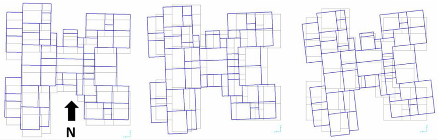
Figure 14. Plan view of the roof level for mode 1 (left), mode 2 (middle), and mode 3 (right) from finite element model.

TABLE 6

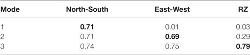
Table 6. Cumulative effective mass participation factors of the finite element model.

Model-Data Comparison

Table 7 shows the comparison of natural frequencies and mode shapes of the FE model and system identification results. In the computation of MAC values, the mode shape components at the SE-N sensors are not used due to the larger estimation error of identified mode shapes at this location. The pairing between modes of the FE model and the identified modes is based on the MAC values of Table 7. Based on the MAC values, it can be concluded that mode 1b from system identification is comparable to mode 1 of the FE model, while mode 1c from system identification is comparable to mode 2 of the FE model. In this table, the MAC values between paired modes are shown in bold. The first two mode shapes of the FE model are also plotted on Figure 12A for comparison. It is worth noting that the FE model cannot represent the identified mode 1a. This is most likely due to modeling simplifications/errors of this complex structure. The identified natural frequencies of modes 1b and 1c are in excellent agreement with model-predicted natural frequencies of the matched modes (i.e., modes 1 and 2 of model). Overall, there is good agreement between the model and the recorded data at the lower frequencies.

TABLE 7

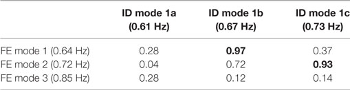
Table 7. Modal Assurance Criterion values between identified (ID) mode shapes and those from finite element (FE) model.

Response Prediction

To examine the performance of the building after the earthquake, the inter-story drift ratios of the different stories are computed using the FE model. These values are compared with the observed damage and surface defect detection results from lidar scans. It is worth highlighting that a linear elastic model is used for the response prediction. Even though the model is linear, the mean displacement demands of linear elastic and inelastic systems are expected to be similar for structures with frequencies below 1 Hz (e.g., Miranda, 1999; Miranda and Ruiz-García, 2002). Figure 15 shows the displacement response spectrum and obtained inter-story drift ratios from the linear time history analysis for the mainshock (M7.8) and aftershock earthquakes (M7.3). As it can be seen in the figure, the lower stories of the building exhibit larger inter-story drift ratios than the upper ones. The range of the maximum inter-story drift ratios from the analysis is between 0.05 to 0.49%. To estimate the damage based on the estimated inter-story drift ratios, the response prediction results are compared to the damage scale proposed by Rossetto and Elnashai (2003). Table 8 lists the expected damage state with corresponding drift limits for infilled RC frames. By comparing the drift ratios from the analysis with the drift limits that provided in Table 8, the expected level of damage for the building after the earthquake is ranged between light to moderate. These results obtained from the FE model correlate well with the lidar assessment of the observed damage on site as shown in Figures 6 and 7 and Table 2.

FIGURE 15

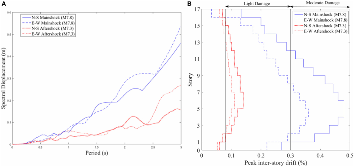
Figure 15. Displacement response spectrum and peak inter-story drift ratios. (A) Displacement response spectrum (5% damping). (B) Peak inter-story drift %.

TABLE 8

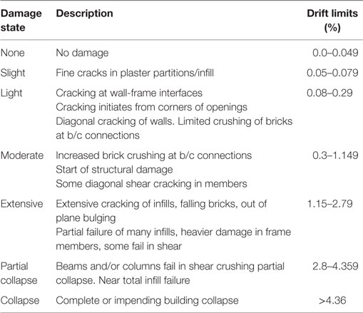
Table 8. Expected damage limit states for infilled reinforced concrete structures [modified from Rossetto and Elnashai (2003)].

Concluding Remarks

This study investigates post-earthquake dynamic performance of an 18-story building in Nepal that was partially damaged during the 2015 Gorkha earthquake and its subsequent aftershocks. The performance is assessed through system identification using ambient vibration measurements, lidar scans for surface defect detection, and FE modeling and response simulation. Modal parameters of the most excited vibration modes of the building are extracted from the measured ambient vibration measurements in the frequency range of 0.2–10 Hz. The natural frequencies are identified accurately and consistently across different subsets of data. The damping ratios are estimated with larger variability but have reasonable values except for the first mode which seems to be inflated. The FAS of measurements reveals the presence of three very closely spaced modes at the frequency of the first identified mode, which is consistent with the FE model. A second modal identification is performed with increased frequency resolution in the frequency range of 0.2–1.0 Hz, and the three closely spaced modes are successfully identified. A linear FE model of the building is also developed, and its modal parameters are compared with those identified from measured data. A good agreement for the first two modes of the FE model with identified modes provides a validation measure for the model. The validated model is used for prediction of structural response to the main earthquake and a major aftershock. Lidar scans of the interior of the structure were collected and analyzed to locate and quantify surface defects. The results of point cloud damage assessment confirm moderate to low damage at lower and higher elevations in comparison to mid-elevations, where more severe damage exhibited by both studied members. These results also comply with predicted response from the FE model.

A few of the lessons learned from this study that may be valuable for other researchers are listed below:

– Natural frequencies of this tall building are identified very accurately even with low amplitude of ambient response and relatively large measurement noise from cables.

– The damping estimates have larger estimation uncertainty compared to the natural frequencies, however, are useful for providing a basis for modeling.

– The closely spaced modes can be missed when identification is performed over a wide frequency range.

– Identification of several modes as a single mode will cause the damping ratio estimate of that mode to be inflated.

– Selection of different reference channels for different modes in the NExT-ERA can improve the accuracy of identification results.

– Using different types of sensors and having unequal signal-to-noise ratio at different channels (due to quality of cables/connectors) will negatively influence the accuracy of mode shape estimates and modal complexities.

– Using a linear FE model to predict the response of the building to earthquake includes some errors as the non-linear behavior cannot be modeled. However, the predictions still provides reasonable accurate estimates for the level and distribution of damage for buildings with primary natural frequency of below 1 Hz.

– The lidar scans of the building provide accurate and quantitative measure of surface defects that are closely correlated with the estimated damage as maximum inter-story drift obtained from the FE model.

Author Contributions

HY performed signal processing and system identification. MAM performed FE modeling and response prediction. MEM performed lidar data processing and surface defect detection. BM supervised the system identification study. AB supervised the FE modeling. AS provided feedback about modeling and identification. RW supervised lidar data processing and defect detection. AB and RW also performed the data collection on site.

Conflict of Interest Statement

The authors declare that the research was conducted in the absence of any commercial or financial relationships that could be construed as a potential conflict of interest.

Funding

Partial support of this study by the National Science Foundation Grants 1254338, 1545632, and 1545595 is gratefully acknowledged. The authors express their gratitude to the building owners who provided access to the buildings and thank Mr. Supratik Bose, Mr. Patrick Burns, Mr. Rajendra Soti, and Mr. Sandip Timsina for their assistance in the collection of data. The opinions, findings, and conclusions expressed in this paper are those of the authors and do not necessarily represent the views of the organizations and collaborators involved in this project.

References

Allemang, R. J., and Brown, D. L. (1982). “A correlation coefficient for modal vector analysis,” in Proceedings of the 1st International Modal Analysis Conference (Orlando: SEM), 110–116.

Google Scholar

Antonacci, E., De Stefano, A., Gattulli, V., Lepidi, M., and Matta, E. (2012). Comparative study of vibration-based parametric identification techniques for a three-dimensional frame structure. Struct. Control Health Monit. 19, 579–608. doi: 10.1002/stc.449

CrossRef Full Text | Google Scholar

Arakawa, T., and Yamamoto, K. (2004). “Frequencies and damping ratios of a high rise building based on microtremor measurement,” in Proc., 13th World Conference on Earthquake Engineering (Vancouver, BC).

Google Scholar

Au, S. K., and Zhang, F. L. (2016). Fundamental two-stage formulation for Bayesian system identification, part I: general theory. Mech. Syst. Signal Process. 66, 31–42. doi:10.1016/j.ymssp.2015.04.025

CrossRef Full Text | Google Scholar

Au, S. K., Zhang, F. L., and Ni, Y. C. (2013). Bayesian operational modal analysis: theory, computation, practice. Comput. Struct. 126, 3–14. doi:10.1016/j.compstruc.2012.12.015

CrossRef Full Text | Google Scholar

Belleri, A., Moaveni, B., and Restrepo, J. I. (2014). Damage assessment through structural identification of a three-story large-scale precast concrete structure. Earthquake Eng. Struct. Dyn. 43, 61–76. doi:10.1002/eqe.2332

CrossRef Full Text | Google Scholar

Brando, G., Rapone, D., Spacone, E., Barbosa, A., Olsen, M., Gillins, D., et al. (2015). “Reconnaissance report on the 2015 Gorkha earthquake effects in Nepal,” in XVI Convegno ANIDIS. L’AQUILA, Italy.

Google Scholar

Brincker, R., and Kirkegaard, P. H. (2010). Editorial for the special issue on operational modal analysis. Mech. Syst. Signal Process. 24, 1209–1212. doi:10.1016/j.ymssp.2010.03.005

CrossRef Full Text | Google Scholar

Brincker, R., Zhang, L., and Andersen, P. (2001). Modal identification of output-only systems using frequency domain decomposition. Smart Mater. Struct. 10, 441–445. doi:10.1088/0964-1726/10/3/303

CrossRef Full Text | Google Scholar

Brownjohn, J. M. W. (2003). Ambient vibration studies for system identification of tall buildings. Earthquake Eng. Struct. Dyn. 32, 71–95. doi:10.1002/eqe.215

CrossRef Full Text | Google Scholar

Brownjohn, J. M. W., Magalhaes, F., Caetano, E., and Cunha, A. (2010). Ambient vibration re-testing and operational modal analysis of the Humber Bridge. Eng. Struct. 32, 2003–2018. doi:10.1016/j.engstruct.2010.02.034

CrossRef Full Text | Google Scholar

Caicedo, J. M., Dyke, S. J., and Johnson, E. A. (2004). Natural excitation technique and eigensystem realization algorithm for phase I of the IASC-ASCE benchmark problem: simulated data. J. Eng. Mech. 130, 49–60. doi:10.1061/(ASCE)0733-9399(2004)

CrossRef Full Text | Google Scholar

Çelebi, M., Okawa, I., Kashima, T., Koyama, S., and Iiba, M. (2014). Response of a tall building far from the epicenter of the 11 March 2011 M 9.0 Great East Japan earthquake and aftershocks. Struct. Des. Tall Spec. Build. 23, 427–441. doi:10.1002/tal.1047

CrossRef Full Text | Google Scholar

Computers and Structures Inc. (2013). SAP2000 V.16 Software. Berkeley: CSI.

Google Scholar

Cunha, A., Caetano, E., Magalhães, F., and Moutinho, C. (2013). Recent perspectives in dynamic testing and monitoring of bridges. Struct. Control Health Monit. 20, 853–877. doi:10.1002/stc.1516

CrossRef Full Text | Google Scholar

Digital Signal Processing Committee of the IEEE, Acoustics, Speech, and Signal Processing Society, eds. (1979). Programs for Digital Signal Processing. New York: IEEE Press.

Google Scholar

FARO. (2011). “Faro laser scanner focus 3D: features, benefits & technical specifications,” FARO Technologies. Lake Mary, FL.

Google Scholar

Federal Emergency Management Agency. FEMA 356. (2000). Prestandard and Commentary for the Seismic Rehabilitation of Buildings. Washington, DC: Federal Emergency Management Agency.

Google Scholar

Feng, M. Q., Kim, J. M., and Xue, H. (1998). Identification of a dynamic system using ambient vibration measurements. J. Appl. Mech. 65, 1010–1021.

Google Scholar

Guldur, B., and Hajjar, J. F. (2014). Laser-Based Structural Sensing and Surface Damage Detection. Report No. NEU-CEE-2014-03. Boston, MA: Department of Civil Engineering, Northeastern University.

Google Scholar

Harris, A., Xiang, Y., Naeim, F., and Zareian, F. (2015). “Identification and validation of natural periods and modal damping ratios for steel and reinforced concrete buildings in California,” in SMIP15 Seminar on Utilization of Strong-Motion Data (Davis), 121–134.

Google Scholar

He, X., Moaveni, B., Conte, J. P., and Elgamal, A. (2006). “Comparative study of system identification techniques applied to New Carquinez Bridge.” in Proceedings of the Third International Conference on Bridge Maintenance, Safety and Management, ed. P. J. d. S. Cruz, D. M. Frangopol, and L. C. C. Neves (Porto: CRC Press), 259–260.

Google Scholar

IS 13920. (1993). Indian Standard, Ductile Detailing of Reinforced Concrete Structures Subjected to Seismic Forces – Code of Practice. New Delhi: Bureau of Indian Standards.

Google Scholar

IS 1893 (part 1). (2002). Indian Standard, Criteria for Earthquake Resistant Design of Structures. New Delhi: Bureau of Indian Standards.

Google Scholar

James, G. H., Carne, T. G., Lauffer, J. P., and Nord, A. R. (1992). “Modal testing using natural excitation,” in Proceedings of the International Modal Analysis Conference (San Diego: SEM Society for Experimental Mechanics Inc.), 1209–1216.

Google Scholar

Jin, S., Lewis, R. R., and West, D. (2005). A comparison of algorithms for vertex normal computation. Vis. Comput. 21, 71–82. doi:10.1007/s00371-004-0271-1

CrossRef Full Text | Google Scholar

Juang, J. N., and Pappa, R. S. (1985). An eigensystem realization algorithm for modal parameter identification and model reduction. J. Guid. Control Dyn. 8, 620–627. doi:10.2514/3.20031

CrossRef Full Text | Google Scholar

Kim, M., Sohn, H., and Chang, C. (2014). Localization and quantification of concrete spalling defects using terrestrial laser scanning. J. Comput. Civ. Eng. 29:04014086. doi:10.1061/(ASCE)CP.1943-5487.0000415

CrossRef Full Text | Google Scholar

Mainstone, R. J. (1971). Summary of paper 7360. On the stiffness and strengths of infilled frames. Proc. Inst. Civ. Eng. 49, 230.

Google Scholar

Miranda, E. (1999). Approximate seismic lateral deformation demands in multistory buildings. ASCE J. Struct. Eng. 125, 417–425.

Google Scholar

Miranda, E., and Ruiz-García, J. (2002). Evaluation of approximate methods to estimate maximum inelastic displacement demands. Earthquake Eng. Struct. Dyn. 31, 539–560. doi:10.1002/eqe.143

CrossRef Full Text | Google Scholar

Moaveni, B., Barbosa, A. R., Conte, J. P., and Hemez, F. M. (2014). Uncertainty analysis of system identification results obtained for a seven story building slice tested on the UCSD-NEES shake table. Struct. Control Health Monit. 21, 466–483. doi:10.1002/stc.1577

CrossRef Full Text | Google Scholar

Pauly, M., Gross, M., and Kobbelt, L. P. (2002). “Efficient simplification of point-sampled surfaces,” in Proceedings of the Conference on Visualization’02 (Boston, MA: IEEE Computer Society), 163–170.

Google Scholar

Peeters, B., and De Roeck, G. (2001). Stochastic system identification for operational modal analysis: a review. J. Dyn. Syst. Meas. Control 123, 659–667. doi:10.1115/1.1410370

CrossRef Full Text | Google Scholar

Pintelon, R., Guillaume, P., and Schoukens, J. (2007). Uncertainty calculation in operational modal analysis. Mech. Syst. Signal Process. 21, 2359–2373. doi:10.1016/j.ymssp.2006.11.007

CrossRef Full Text | Google Scholar

Rai, D. C., Singhal, V., Raj, S. B., and Sagar, S. L. (2015). Reconnaissance of the effects of the M7.8 Gorkha (Nepal) earthquake of April 25, 2015. Geomatics Nat. Hazards Risk 7, 1–17. doi:10.1080/19475705.2015.1084955

CrossRef Full Text | Google Scholar

Reynders, E., Pintelon, R., and De Roeck, G. (2008). Uncertainty bounds on modal parameters obtained from stochastic subspace identification. Mech. Syst. Signal Process. 22, 948–969. doi:10.1016/j.ymssp.2007.10.009

CrossRef Full Text | Google Scholar

Rossetto, T., and Elnashai, A. (2003). Derivation of vulnerability functions for European-type RC structures based on observational data. Eng. Struct. 25, 1241–1263. doi:10.1016/S0141-0296(03)00060-9

CrossRef Full Text | Google Scholar

Saneinejad, A., and Hobbs, B. (1995). Inelastic design of infilled frames. J. Struct. Eng. Asce 121, 634–650. doi:10.1061/(Asce)0733-9445(1995)121:4(634)

CrossRef Full Text | Google Scholar

Satake, N., Suda, K. I., Arakawa, T., Sasaki, A., and Tamura, Y. (2003). Damping evaluation using full-scale data of buildings in Japan. J. Struct. Eng. 129, 470–477. doi:10.1061/(ASCE)0733-9445(2003)129:4(470)

CrossRef Full Text | Google Scholar

Shakarji, C. M. (1998). Least-squares fitting algorithms of the NIST algorithm testing system. J. Res. Nat. Inst Stand. Technol. 103, 633–641. doi:10.6028/jres.103.043

PubMed Abstract | CrossRef Full Text | Google Scholar

Sim, S. H., Spencer, B. F., Zhang, M., and Xie, H. (2010). Automated decentralized modal analysis using smart sensors. Struct. Control Health Monit. 17, 872–894. doi:10.1002/stc.348

CrossRef Full Text | Google Scholar

Siringoringo, D. M., and Fujino, Y. (2008). System identification of suspension bridge from ambient vibration response. Eng. Struct. 30, 462–477. doi:10.1016/j.engstruct.2007.03.004

CrossRef Full Text | Google Scholar

Stafford Smith, B., and Carter, C. (1969). A method of analysis for infilled frames. Proc. Inst. Civ. Eng. 44, 31–48.

Google Scholar

Van Overschee, P., and de Moore, B. (1996). Subspace Identification for Linear Systems. Massachusetts, USA: Kluer Academic Publishers.

Google Scholar

Verboven, P., Parloo, E., Guillaume, P., and Van Overmeire, M. (2002). Autonomous structural health monitoring – part 1: modal parameter estimation and tracking. Mech. Syst. Signal Process. 16, 637–657. doi:10.1006/mssp.1492

CrossRef Full Text | Google Scholar

Yu, H. (2016). Post-Earthquake System Identification of an 18-Story RC Building in Nepal. Master’s thesis, Department of Civil and Environmental Engineering, Tufts University, Massachusetts.

Google Scholar

Zhang, F. L., and Au, S. K. (2016). Fundamental two-stage formulation for Bayesian system identification, part II: application to ambient vibration data. Mech. Syst. Signal Process. 66, 43–61. doi:10.1016/j.ymssp.2015.04.024

CrossRef Full Text | Google Scholar