Critical Steady-State Response of Single-Degree-of-Freedom Bilinear Hysteretic System under Multi Impulse as Substitute of Long-Duration Ground Motion

Introduction

The classification of earthquake ground motions has often been conducted (Abrahamson et al., 1998). One is a near-fault ground motion and another one is a long-duration (mostly far-fault) ground motion. The soil types (soil, rock) of recording sites and types of fault mechanisms are other factors for classification. In addition to these two representative ground motions, long-period ground motions were observed rather recently (Takewaki et al., 2011). The effects of near-fault ground motions on structural responses have been investigated from various viewpoints (for example, Bertero et al., 1978; Kalkan and Kunnath, 2006). The terminologies of fling-step and forward-directivity are widely used for characterizing such near-fault ground motions. Northridge earthquake in 1994, Hyogoken-Nanbu (Kobe) earthquake in 1995, Chi-Chi (Taiwan) earthquake in1999, and Kumamoto earthquake in 2016 drew special attention to many earthquake structural engineers.

The fault-parallel fling-step and fault-normal forward-directivity inputs have been analyzed as two or three wavelets. Most of the past works on the near-fault ground motions treat mainly the elastic response. This may result from the fact that the number of parameters (e.g., duration, period and amplitude of pulse, ratio of pulse frequency to structure natural frequency, change of equivalent natural frequency for the increased input level) to be considered is large and the numerical analysis itself of elastic–plastic response is quite complicated.

To overcome such complex problem, a smart approach based on an innovative tool, i.e., the double impulse, was introduced by Kojima and Takewaki (2015a). The double impulse represents approximately the fling-step near-fault ground motion and a closed-form maximum elastic–plastic response of a structure under the “critical double impulse” was derived. It was shown that, since only the free-vibration exists under such double impulse, the energy balance approach plays a key role in the derivation of such closed-form expression. It was also demonstrated that the maximum elastic–plastic deformation can occur either after the first or second impulse depending on the input level. The reliability of the proposed theory was confirmed through the comparison with the results of time-history response analysis to the corresponding one-cycle sine wave which is a representative of the fling-step near-fault ground motion. The intensity of the double impulse was controlled so that its maximum Fourier amplitude becomes equivalent to that of the corresponding one-cycle sine wave. The theory for the fling-step input was extended to the forward-directivity input by Kojima and Takewaki (2015b).

The closed-form expressions of the elastic–plastic earthquake response have been derived so far only for the steady-state and transient responses to a sine wave (Caughey, 1960a,b; Roberts and Spanos, 1990; Liu, 2000). It should be noted that the forced input by the sine wave brought a complexity for a simple solution of resonant and non-resonant responses. It may be a natural inspiration that, if a long-duration ground motion can be simplified into a multiple impulse, the elastic–plastic response (expressed as continuation of free-vibrations) can be derived by an energy balance approach without solving directly the differential equation.

In the long history of earthquake-resistant design since the 20th century, the resonance played a key role in the phase of damage analysis of structures and it has been investigated extensively. Generally, the resonant equivalent frequency has to be analyzed for a specified input level by changing the input frequency in a parametric manner in dealing with the response to a sine wave (Caughey, 1960a,b; Iwan, 1961, 1965a,b; Roberts and Spanos, 1990; Liu, 2000). It is therefore preferable that no iteration is required, and this can be performed by introducing the multi impulse input. In the multi impulse input, the analysis can be done without the specification of input frequency (timing of impulses) before the second impulse is input. The resonance can be analyzed by using an energy balance approach and the timing of the impulses can be obtained as the time with zero restoring force. The maximum elastic–plastic response after impulse can be obtained by equating the initial kinetic energy given by the initial velocity to the sum of hysteretic and elastic strain energies. It should be pointed out that only critical response is focused by the proposed method, and the critical resonant frequency can be derived automatically for the increasing input level of the multi impulse.

In the previous paper (Kojima and Takewaki, 2015c), a closed-form expression of the critical response of an elastic–perfectly plastic single-degree-of-freedom (SDOF) model under multiple impulse input was derived. However, the elastic–plastic model with bilinear hysteresis has a stable response characteristic and the steady-state response of such model is of great importance from the viewpoint of the comparison with the result by the previous works (Caughey, 1960a,b; Iwan, 1961). Furthermore, the elastic–plastic model with bilinear hysteresis possesses other types of complexity and its investigation is highly desired.

Figure 1 shows an actual example of the resonant response recorded in a high-rise building in Osaka, Japan, during the 2011 off the Pacific coast of Tohoku earthquake. Although damage was observed in only non-structural components in this building, the development of damage in structural components should be taken into account from the viewpoint of resilience. This actual incident clearly implies the warning to consider carefully the response under long-duration ground motion.

FIGURE 1

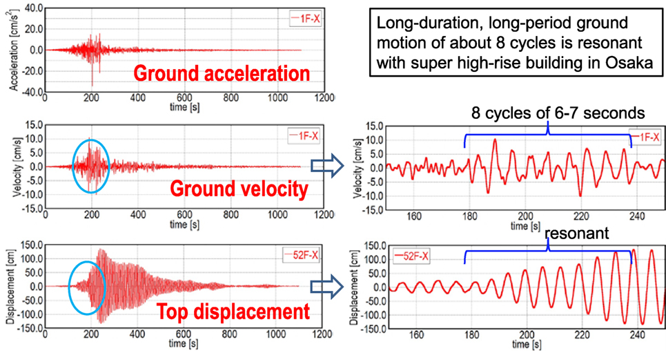
Figure 1. Resonant response of a super high-rise building in Osaka, Japan, during the 2011 off the Pacific coast of Tohoku earthquake under long-duration, long-period ground motion (Takewaki et al., 2011).

In this paper, the multi impulse input is introduced as a substitute of the multi-cycle sinusoidal wave which represents the long-duration ground motion and a closed-form expression is derived of the elastic–plastic steady-state response of an SDOF structure with bilinear hysteresis under the “critical multi impulse input”. An undamped bilinear hysteretic SDOF system used in this paper is explained in Section “Bilinear Hysteretic SDOF System.” The closed-form expressions are derived of the elastic–plastic steady-state responses under the critical multi impulse and the critical time intervals of two cases in Section “Closed-Form Expression of Elastic–Plastic Steady-state Response under Critical Multi Impulse.” CASE 1 is the case where each impulse acts at the zero restoring-force timing in the unloading process and the other case, CASE 2, is the case where each impulse acts at the zero restoring-force timing in the loading process. It is investigated whether the response under the multi impulse with the critical time interval obtained in Section “Closed-Form Expression of Elastic–Plastic Steady-state Response under Critical Multi Impulse” converges to the steady state in which each impulse acts at the zero restoring-force point in Section “Convergence of Impulse Timing.” The accuracy of using the multi impulse as a substitute of the long-duration ground motion is checked through the comparison with the response under the corresponding multi-cycle sinusoidal wave in Section “Accuracy Check by Time-History Response Analysis under the Corresponding Multi-Cycle Sinusoidal Wave.” The validity of the critical time interval obtained in Section “Closed-Form Expression of Elastic–Plastic Steady-state Response under Critical Multi Impulse” is confirmed by time-history response analysis of the SDOF bilinear hysteresis system under multi impulse with various impulse time intervals in Section “Proof of Critical Timing.” The applicability of the critical impulse timing obtained in Section “Closed-Form Expression of Elastic–Plastic Steady-state Response under Critical Multi Impulse” to the corresponding sinusoidal wave is investigated in Section “Applicability of Critical Multi Impulse Timing to Corresponding Sinusoidal Wave.” The accuracy of the proposed closed-form steady-state response under the critical multi impulse is also investigated in Section “Accuracy Check by Exact Solution Subjected to the Corresponding Multi-Cycle Sinusoidal Wave” through the comparison with the resonance curve under the sinusoidal wave provided by Iwan (1961). The conclusions are summarized in Section “Conclusion.”

Bilinear Hysteretic SDOF System

Consider an undamped bilinear hysteretic SDOF system of mass m and stiffness k subjected to the multi impulse with the equal time interval as shown in Figure 2A,B. V is the given initial velocity (the input velocity level of each impulse) and t₀ is the equal time interval between two consecutive impulses. The ratio of the post-yield stiffness to the initial elastic stiffness is expressed by α. In this paper, α > 0. The yield deformation and the yield force are denoted by d_y and f_y. Let ${\mathrm{\omega }}_1=\sqrt{k/m}$, u and f denote the undamped natural circular frequency, the displacement of the mass relative to the ground (deformation of the system), and the restoring force of the model, respectively. The time derivative is denoted by an overdot. In Section “Closed-Form Expression of Elastic–Plastic Steady-state Response under Critical Multi Impulse,” these parameters will be treated as normalized ones to capture the intrinsic relation between the input parameters and the elastic–plastic response. However, numerical investigations will be made in Sections “Convergence of Impulse Timing,” “Accuracy Check by Time-History Response Analysis under the Corresponding Multi-Cycle Sinusoidal Wave,” “Proof of Critical Timing,” “Applicability of Critical Multi Impulse Timing to Corresponding Sinusoidal Wave,” and “Accuracy Check by Exact Solution Subjected to the Corresponding Multi-Cycle Sinusoidal Wave” to demonstrate an example of actual parameters.

FIGURE 2

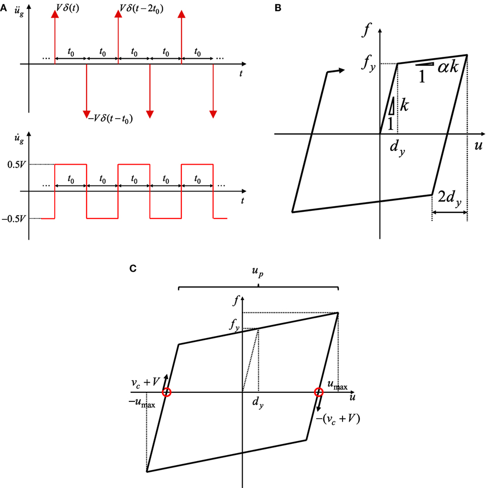
Figure 2. Impulse input and bilinear hysteretic restoring-force deformation characteristic: (A) multi impulse with equal time interval t₀, (B) bilinear hysteretic restoring-force characteristic, (C) steady-state loop under critical multi impulse.

Closed-Form Expression of Elastic–Plastic Steady-State Response Under Critical Multi Impulse

In the previous works (Kojima and Takewaki, 2015a,b,c), some closed-form expressions of the critical elastic–plastic response of an SDOF elastic–perfectly plastic system under the double, triple, and multi impulse have been derived. A closed-form expression of the maximum deformation of an SDOF bilinear hysteretic system under the double impulse has also been derived (Kojima and Takewaki, 2016). In this paper, a closed-form expression of the steady-state elastic–plastic response of an SDOF bilinear hysteretic system under the critical multi impulse is derived.

The response after each impulse input can be expressed by the instantaneous change of velocity of the structural mass by V and only free vibration appears after each impulse input. Since the elastic–plastic response of the SDOF bilinear hysteretic system under the multi impulse can be expressed by the continuation of free vibrations, the plastic deformation amplitude and the maximum deformation can be derived by an energy approach without solving directly the equation of motion. The kinetic energy introduced at the input time of each impulse is transformed into the combination of the hysteretic energy and the strain energy. It should be remarked that each impulse’s critical timing corresponds to the phase with the zero restoring force and a kinetic energy alone appears in this phase as mechanical energies. By using this rule, the maximum deformation can be obtained in a simple manner. In the previous paper (Kojima and Takewaki, 2015c), the closed-form expression of plastic deformation amplitude and the critical timing of the elastic–perfectly plastic SDOF system under the critical multi impulse have been derived. In order to derive the closed-form plastic deformation amplitude and critical timing, a modified multi impulse, in which the first and second impulses are modified so that the second impulse is given at the zero restoring force, was introduced in the study by Kojima and Takewaki (2015c). However, the elastic–plastic response of the present SDOF bilinear hysteretic system with α > 0 cannot become stable under the first few impulses even in the condition that each impulse acts at the zero restoring force and the response converges to a steady state as shown in Figure 2C after a sufficiently large number of repetitive impulses. In this section, the steady state in which each impulse acts at the zero restoring-force point is assumed and the closed-form expressions of the elastic–plastic response and the critical timing are derived by using the assumption of the steady state and the energy approach. The convergence of the response under the multi impulse with the equal time interval obtained in Section “Derivation of Critical Impulse Timing” into the steady state will be verified in Section “Convergence of Impulse Timing.” The convergence of the response under a harmonic wave into the steady state was also confirmed in the previous paper (Iwan, 1961).

The steady state under the critical multi impulse can be classified into two cases depending on the plastic deformation level as shown in Figures 3A,B. Figures 3A,B show the case (CASE 1) that each impulse acts at the zero restoring-force timing in the unloading process and the case (CASE 2) that each impulse acts at the zero restoring-force timing in the loading process, respectively. The boundary between CASE 1 and CASE 2 is given by $u_p/d_y=2/\mathrm{\alpha }$ and this condition will be derived in Section “Case 1: Impulse in Unloading Process.”

FIGURE 3

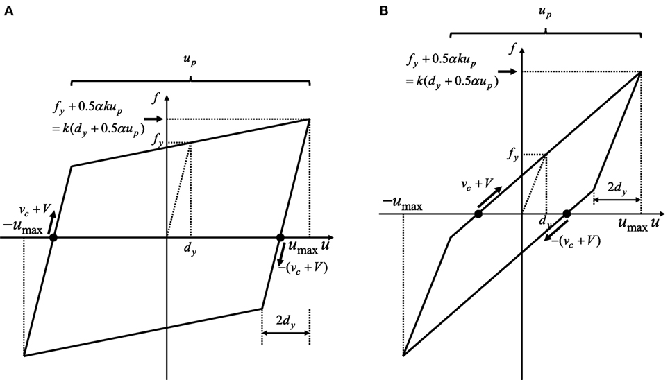
Figure 3. Restoring-force deformation relation under critical multi impulse: (A) CASE 1 $\left(u_p/d_y\le 2/\mathrm{\alpha }\right)$: impulse in unloading process; (B) CASE 2 $\left(u_p/d_y>2/\mathrm{\alpha }\right)$: impulse in loading process.

CASE 1: Impulse in Unloading Process

Consider CASE 1. The steady-state elastic–plastic response (plastic deformation amplitude and maximum deformation) is derived of the SDOF bilinear hysteretic system under the critical multi impulse by using the energy balance law. Figure 4A shows the derivation of the maximum steady-state response in CASE 1 based on the energy approach. Figures 4B,C present the time histories of the deformation and the restoring force in the steady state with the time interval $t_0^c$ between two consecutive impulses. t_AB, t_BC, t_CD denote the time intervals between point A, B, point B, C, and point C, D, respectively, in Figure 4A. The closed-form expressions of the time-history responses of the deformation and the restoring force in the steady state with the critical time interval $t_0^c\left(=t_{\mathit{AB}}+t_{\mathit{BC}}+t_{\mathit{CD}}\right)$ between two consecutive impulses can be obtained by solving the differential equations (equations of motion) and substituting the continuation conditions at the transition points (point A, B, and C). The closed-form expressions of the time-history responses and the critical time interval are derived in Sections “Derivation of Critical Impulse Timing” and Appendix 1.

FIGURE 4

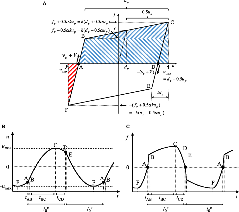
Figure 4. Derivation of maximum deformation under critical multi impulse based on energy approach: (A) restoring-force deformation relation; (B) displacement time history; (C) restoring-force time history (CASE 1: $V/V_y<-2+2\sqrt{1/\mathrm{\alpha }}$).

The velocity v_c at the zero restoring-force point in the unloading process (point A in Figure 4) can be derived by using the energy balance law. The energy balance law between the starting point of unloading (point F in Figure 4) and the zero restoring-force point (point A in Figure 4) is expressed by

$k{\left(d_y+0.\mathrm{5\alpha }{u}_p\right)}^2/2={\mathit{mv}}_c^2/2$ (1)

The left-hand side of Eq. 1 expresses the elastic strain energy shown by the red shaded area in Figure 4A. On the other hand, the right-hand side of Eq. 1 indicates the kinetic energy at the zero restoring-force point.

From Eq. 1, v_c is expressed with u_p by

$v_c/V_y=1+0.\mathrm{5\alpha }\left(u_p/d_y\right)$ (2)

where V_y = ω₁d_y. V_y denotes the input level of the single impulse at which the SDOF system just attains the yield deformation after the single impulse. This parameter also presents a strength parameter with velocity dimension.

The plastic deformation u_p after each impulse can be obtained from the energy balance law. The energy balance law between the zero restoring-force point (point A in Figure 4) and the point attaining the maximum deformation (point C in Figure 4) can be described by

$m{\left(v_c+V\right)}^2/2=k{\left(d_y-0.\mathrm{5\alpha }{u}_p\right)}^2/2+\mathrm{\alpha }k{u}_p^2/2+\left(f_y-0.\mathrm{5\alpha }k{u}_p\right)u_p$ (3)

The left-hand side of Eq. 3 expresses the kinetic energy computed in terms of the velocity (v_c + V) of mass just after each impulse. On the other hand, the right-hand side of Eq. 3 indicates the hysteretic and elastic strain energy shown by the blue shaded area in Figure 4A.

Substitution of Eq. 2 into Eq. 3 and rearrangement of the resulting equation provide

$u_p/d_y=\mathrm{\{}{\left(V/V_y\right)}^2+2\left(V/V_y\right)\mathrm{\}}/\mathrm{\{}2-\mathrm{2\alpha }-\mathrm{\alpha }\left(V/V_y\right)\mathrm{\}}$ (4)

From Eq. 4 and Figure 4A, u_max can be obtained as follows:

$u_{\text{max}}/d_y=1+0.5\left(u_p/d_y\right)=1+0.5\left[\mathrm{\{}{\left(V/V_y\right)}^2+2\left(V/V_y\right)\mathrm{\}}/\mathrm{\{}2-\mathrm{2\alpha }-\mathrm{\alpha }\left(V/V_y\right)\mathrm{\}}\right]$ (5)

Consider the boundary between CASE 1 and CASE 2. In this boundary, the zero restoring-force point (point A in Figure 4) is equal to the point of the yielding initiation (point B in Figure 4) and each impulse acts at this point (point A in Figure 5A). Figures 5A,B show the derivation of the maximum steady-state response in this boundary case based on the energy approach. The plastic deformation in this boundary case can be obtained from Figure 5A.

$f_y+0.\mathrm{5\alpha }k{u}_p=2f_y$ (6)

FIGURE 5

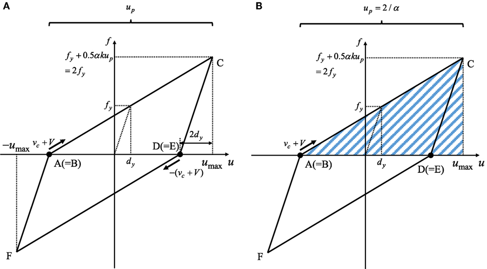
Figure 5. Restoring-force deformation relation in the boundary case between CASE 1 and CASE 2: (A) acting points of each impulse; (B) sum of hysteretic and elastic strain energy after each impulse.

From Eq. 6, u_p in this boundary case can be obtained as follows:

$u_p/d_y=2/\mathrm{\alpha }$ (7)

The boundary input velocity level of the multi impulse is derived next. From Eq. 7 and Figure 5B, the velocity v_c at the zero restoring-force point (point A in Figure 5A) can be derived by using the energy balance law. The energy balance law between the starting point of unloading (point F in Figure 5B) and the zero restoring-force point (point A in Figure 5B) can be expressed by

$k{\left(2d_y\right)}^2/2={\mathit{mv}}_c^2/2$ (8)

The left-hand side of Eq. 8 indicates the elastic strain energy at the starting point of unloading. On the other hand, the right-hand side of Eq. 8 expresses the kinetic energy at the zero restoring-force point.

From Eq. 8, v_c can be obtained as follows:

$v_c/V_y=2$ (9)

The energy balance law between the zero restoring-force point (point A in Figure 5B) and the point attaining the maximum deformation (point C in Figure 5B) is also expressed by

$m{\left(v_c+V\right)}^2/2=\mathrm{\alpha }k{u}_p^2/2$ (10)

The left-hand side of Eq. 10 indicates the kinetic energy computed in terms of the velocity (v_c + V) of mass just after each impulse. On the other hand, the right-hand side of Eq. 10 expresses the hysteretic and elastic strain energy shown by the blue shaded area in Figure 5B.

Substitution of Eqs 7 and 9 into Eq. 10 and rearrangement of the resulting equation provide the boundary input velocity level as follows:

$V/V_y=-2+2\sqrt{1/\mathrm{\alpha }}$ (11)

CASE 2: Impulse in Loading Process (Second Stiffness Range)

Consider next CASE 2 $\left(V/V_y>-2+\sqrt{1/\mathrm{\alpha }}\right)$. The steady-state elastic–plastic response is derived of the SDOF bilinear hysteretic system under the critical multi impulse by using the energy balance law. Figure 6A shows the maximum steady-state response in CASE 2 based on the energy approach. Figures 6B,C present the one-cycle time histories of the deformation and the restoring force between two consecutive impulses in the steady state. t_AB, t_BC, t_CD denote the time intervals between point A, B, point B, C, and point C, D, respectively, in Figure 6A. The closed-form expressions of the time-history responses of the deformation and the restoring force in the steady state with the critical time interval $t_0^c\left(=t_{\mathit{AB}}+t_{\mathit{BC}}+t_{\mathit{CD}}\right)$ between two consecutive impulses can be obtained by solving the differential equations and substituting the continuation conditions at the transition points (point A, B, and C). The closed-form expressions of the time-history responses and the critical time interval are derived in Section “Derivation of Critical Impulse Timing” and Appendix 1.

FIGURE 6

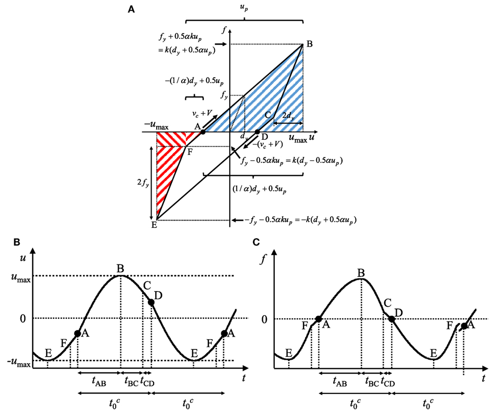
Figure 6. Derivation of maximum deformation under critical multi impulse based on energy approach: (A) restoring-force deformation relation; (B) displacement time history; (C) restoring-force time history (CASE 2: $V/V_y\ge -2+2\sqrt{1/\mathrm{\alpha }}$).

The velocity v_c at the zero restoring-force point in the loading process (point A in Figure 6) can be derived by using the energy balance law. The energy balance law between the starting point of unloading (point E in Figure 6) and the zero restoring-force point (point A in Figure 6) can be expressed by

$k{\left(2d_y\right)}^2/2+\left(-f_y+0.\mathrm{5\alpha }k{u}_p\right)\left(2d_y\right)+\left(\mathrm{\alpha }k\right){\mathrm{\{}\left(-f_y+0.\mathrm{5\alpha }k{u}_p\right)/\left(\mathrm{\alpha }k\right)\mathrm{\}}}^2/2=m{v}_c^2/2$ (12)

The left-hand side of Eq. 12 indicates the elastic strain energy shown by the red shaded area in Figure 6A. On the other hand, the right-hand side of Eq. 12 expresses the kinetic energy at the zero restoring-force point.

From Eq. 12, v_c can be expressed with u_p by

$v_c/V_y=\sqrt{\left(\mathrm{\alpha }/4\right){\left(u_p/d_y\right)}^2+\left(\mathrm{2\alpha }-1\right)\left(u_p/d_y\right)+\left(1/\mathrm{\alpha }\right)}$ (13)

The plastic deformation u_p after each impulse can be obtained from the energy balance law. The energy balance law between the zero restoring-force point (point A in Figure 6) and the point attaining the maximum deformation (point B in Figure 6) can be expressed by

$m{\left(v_c+V\right)}^2/2=\mathrm{\alpha }k{\mathrm{\{}\left(f_y+0.\mathrm{5\alpha }k{u}_p\right)/\left(\mathrm{\alpha }k\right)\mathrm{\}}}^2/2$ (14)

The left-hand side of Eq. 14 indicates the kinetic energy computed by the velocity (v_c + V) of mass just after each impulse. On the other hand, the right-hand side of Eq. 14 expresses the hysteretic and elastic strain energy shown by the blue shaded area in Figure 6A.

Substitution of Eq. 13 into Eq. 14 and rearrangement of the resulting equation provide

$u_p/d_y=\mathrm{\{}{\left(V/V_y\right)}^2-2\left(V/V_y\right)/\sqrt{\mathrm{\alpha }}\mathrm{\}}/\mathrm{\{}\mathrm{2\alpha }-2+\sqrt{\mathrm{\alpha }}\left(V/V_y\right)\mathrm{\}}$ (15)

From Eq. 15 and Figure 6A, u_max can be obtained as follows:

$u_{\text{max}}/d_y=1+0.5\left(u_p/d_y\right)=1+0.5\left[\mathrm{\{}{\left(V/V_y\right)}^2-2\left(V/V_y\right)/\sqrt{\mathrm{\alpha }}\mathrm{\}}/\mathrm{\{}\mathrm{2\alpha }-2+\sqrt{\mathrm{\alpha }}\left(V/V_y\right)\mathrm{\}}\right]$ (16)

From Eq. 15 or 16, the elastic–plastic response diverges to infinity under the condition that $\mathrm{2\alpha }-2+\sqrt{\mathrm{\alpha }}\left(V/V_y\right)=0$. In CASE 2, the impulse input velocity level at which the response diverges can be obtained by $\mathrm{2\alpha }-2+\sqrt{\mathrm{\alpha }}\left(V/V_y\right)=0$ as follows:

$V/V_y=\left(-\mathrm{2\alpha }+2\right)/\sqrt{\mathrm{\alpha }}$ (17)

The response divergence phenomenon can occur under the condition $V/V_y\ge \left(-\mathrm{2\alpha }+2\right)/\sqrt{\mathrm{\alpha }}$ because the increment of the input energy due to the repetitive impulses cannot be consumed by plastic deformation. The same phenomenon can be observed under a sinusoidal wave input (Iwan, 1961).

From Eqs 11 and 17, the input velocity level in CASE 2 has to satisfy the following inequality.

$-2+2\sqrt{1/\mathrm{\alpha }}<V/V_y<\left(-\mathrm{2\alpha }+2\right)/\sqrt{\mathrm{\alpha }}$ (18)

Results in Numerical Example

The plastic deformation amplitudes u_p/d_y obtained in Sections “Case 1: Impulse in Unloading Process” and “Case 2: Impulse in Loading Process (Second Stiffness Range)” are shown in Figures 7A,B. Figure 7A shows the plastic deformation amplitude u_p/d_y with respect to the input velocity level V/V_y for various post-yield stiffness ratios α = 0, 0.1, 0.2, 0.3, 0.4, 0.5, 0.6, 0.7, 0.8, 0.9. On the other hand, Figure 7B presents the plastic deformation amplitude u_p/d_y with respect to the post-yield stiffness ratio α for various input velocity levels V/V_y = 0.1, 0.5, 1.0, 1.5. The model with α = 0 is equivalent to the elastic–perfectly plastic model and u_p/d_y for this model has been derived in the previous paper (Kojima and Takewaki, 2015c).

FIGURE 7

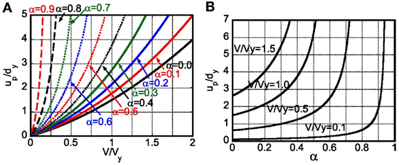
Figure 7. Plastic deformation amplitude u_p/d_y under critical multi impulse: (A) u_p/d_y with respect to input level V/V_y for various post-yield stiffness ratio α, (B) u_p/d_y with respect to post-yield stiffness ratio α for various input levels V/V_y.

Derivation of Critical Impulse Timing

The time intervals between two consecutive impulses in CASE 1 and CASE 2 are derived in this section. In CASE 1 and CASE 2, each impulse acts at the zero restoring-force point. The time interval $t_0^c$ between two consecutive impulses can be obtained by solving the differential equations (equations of motion) and substituting the continuation conditions at the transition points. The time interval $t_0^c$, shown in Figures 4B and 6B, can be expressed as follows:

$\begin{array}{l}\frac{t_0^c}{T_1}=\frac{1}{\mathrm{2\pi }}\left[\arcsin \left\{\frac{1-0.\mathrm{5\alpha }\left(u_p/d_y\right)}{\left(v_c+V\right)/V_y}\right\}+\frac{1}{\sqrt{\mathrm{\alpha }}}\arctan \left\{\frac{1}{\sqrt{\mathrm{\alpha }}}\frac{v_B/V_y}{\left(1/\mathrm{\alpha }\right)-0.5\left(u_p/d_y\right)}\right\}\right]+\frac{1}{4}\hfill \\ \text{for }V/V_y\le -2+2\sqrt{1/\mathrm{\alpha }}\hfill \end{array}$ (19a)

$\begin{array}{l}\frac{t_0^c}{T_1}=\frac{1}{4}\left(1+\frac{1}{\sqrt{\mathrm{\alpha }}}\right)+\frac{1}{\mathrm{2\pi }}\left[-\arcsin \left\{\frac{0.\mathrm{5\alpha }\left(u_p/d_y\right)-1}{0.\mathrm{5\alpha }\left(u_p/d_y\right)+1}\right\}+\frac{1}{\sqrt{\mathrm{\alpha }}}\arctan \left\{\frac{0.5\left(u_p/d_y\right)-\left(1/\mathrm{\alpha }\right)}{\sqrt{2\left(u_p/d_y\right)}}\right\}\right]\hfill \\ \text{for }V/V_y>-2+2\sqrt{1/\mathrm{\alpha }}\hfill \end{array}$ (19b)

The quantities u_p/d_y and v_c/V_y in Eq. 19a are obtained from Eqs 4 and 2 and u_p/d_y in Eq. 19b is obtained from Eq. 15. In addition, the velocity v_B/V_y at point B in Eq. 19a is obtained by

$v_B/V_y=\sqrt{{\mathrm{\{}\left(v_c+V\right)/V_y\mathrm{\}}}^2-{\mathrm{\{}1-0.\mathrm{5\alpha }\left(u_p/d_y\right)\mathrm{\}}}^2}\text{for }V/V_y\le -2+2\sqrt{1/\mathrm{\alpha }}$ (20)

The detailed derivation of Eqs 19a, 19b, and 20 is shown in Appendix 1.

Figure 8 shows the normalized quantity of the time interval $t_0^c$ with respect to the input velocity level for various post-yield stiffness ratios α = 0, 0.1, 0.2, 0.3. The model with α = 0 is equivalent to the elastic–perfectly plastic model and $t_0^c$ in this model was derived in the previous paper (Kojima and Takewaki, 2015c).

FIGURE 8

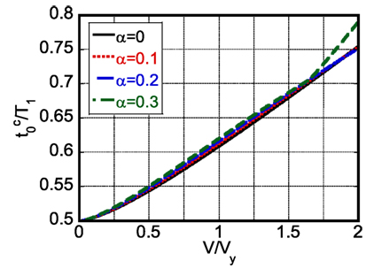
Figure 8. Critical impulse timing $t_0^c/T_1$ with respect to input level V/V_y for various post-yield stiffness ratios α.

Convergence of Impulse Timing

In this section, it is investigated whether the response under the multi impulse with the equal time interval $t_0^c$ obtained in Section “Derivation of Critical Impulse Timing” converges to the steady state in which each impulse acts at the zero restoring-force point as shown in Figure 3. The closed-form expression of the time-history response in the steady state can be derived (see Appendix 1). However, the transient response is complicated because the number of impulses for convergence depends on the input velocity level and the post-yield stiffness ratio. The time-history response analysis is used to calculate the response under the multi impulse with the time interval $t_0^c$. T₁ = 1.0 (s), d_y = 0.04 (m), Δt = 1.0 × 10⁻⁴T₁ are used in the analysis. Δt denotes the time increment used in the time-history response analysis. The response under the multi impulse is calculated by adding ±V to the velocity of the mass at the impulse timing. Figures 9–11 show the time histories of relative displacement, relative velocity, restoring force, and restoring-force deformation relation under the multi impulse with the time interval $t_0^c$ in the model with α = tan(π/8) = 0.414 for V/V_y = 0.5, 1.0, 1.5. This post-yield stiffness ratio was taken from the previous work (Iwan, 1961). It should be noted that the time interval used in this section is obtained by using the assumption of the steady state. The circles in Figures 9–11 indicate the acting points of impulses. It can be observed that the response converges to a state in which each impulse acts at the zero restoring force irrespective of the input velocity level and the maximum deformation and the plastic deformation amplitude after convergence correspond to the closed-form expressions obtained in Sections “Case 1: Impulse in Unloading Process” and “Case 2: Impulse in Loading Process (Second Stiffness Range).” In the model with α = tan(π/8) = 0.414, the input velocity levels V/V_y = 0.5, 1.0 correspond to CASE 1 in Section “Case 1: Impulse in Unloading Process” and the acting points of impulses converge to the zero restoring-force timing in the unloading process in Figures 9 and 10. From Figures 9 and 10, the required number of impulses is about 25. On the other hand, the input velocity level V/V_y = 1.5 corresponds to CASE 2 in Section “Case 2: Impulse in Loading Process (Second Stiffness Range)” and the acting points of impulses converge to the zero restoring-force timing in the loading process in Figure 11. From Figure 11, CASE 2 requires over 100 impulses for convergence.

FIGURE 9

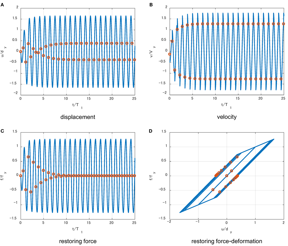
Figure 9. Response under multi impulse with time interval $t_0^c$ for V/V_y = 0.5 and α = tan(π/8) = 0.414 (impulse timing is the critical one obtained by steady-state assumption): (A) displacement, (B) velocity, (C) restoring force, and (D) restoring-force deformation relation.

FIGURE 10

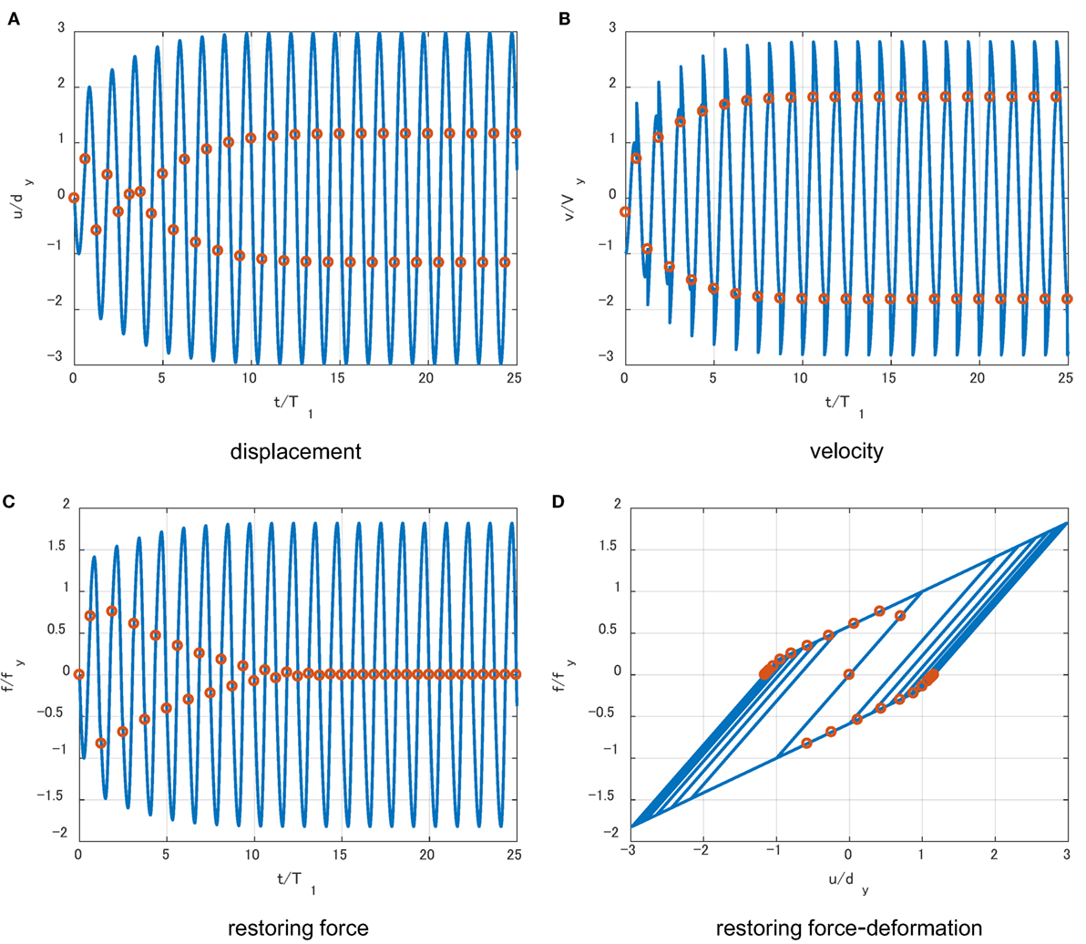
Figure 10. Response under multi impulse with time interval $t_0^c$ for V/V_y = 1.0 and α = tan(π/8) = 0.414 (impulse timing is the critical one obtained by steady-state assumption): (A) displacement, (B) velocity, (C) restoring force, and (D) restoring-force deformation relation.

FIGURE 11

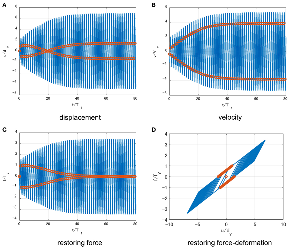
Figure 11. Response under multi impulse with time interval $t_0^c$ for V/V_y = 1.5 and α = tan(π/8) = 0.414 (impulse timing is the critical one obtained by steady-state assumption): (A) displacement, (B) velocity, (C) restoring force, and (D) restoring-force deformation relation.

Accuracy Check by Time-History Response Analysis Under the Corresponding Multi-Cycle Sinusoidal Wave

In order to check the accuracy of using the multi impulse with the equal time interval as a substitute of the corresponding multi-cycle sinusoidal wave representing long-duration ground motions, the time-history response analysis of the SDOF bilinear hysteresis system under the corresponding multi-cycle sinusoidal wave is conducted.

In the evaluation procedure, it is important to adjust the input level of the multi impulse and the corresponding multi-cycle sinusoidal wave based on the equivalence of the maximum Fourier amplitude. The period, the circular frequency, the acceleration amplitude, and the velocity amplitude of the corresponding sinusoidal wave are denoted by T_l, ω_l = 2π/T_l, A_l, and V_l = A_l/ω_l, respectively, and $T_l=2t_0^c$ is used in this section. The number of cycles of the multi-cycle sinusoidal wave is half of the number of impulses. In the derivation of the response under the multi impulse, the steady state after a sufficient number of impulses is assumed as shown in Figures 9–11. The relation between the input velocity level of the multi impulse with the sufficient number of impulses (for example over 20 impulses) and the acceleration amplitude of the corresponding multi-cycle sinusoidal wave with the sufficient number of cycles is expressed as follows:

$V_l=A_l/{\mathrm{\omega }}_l=\left(2/\mathrm{\pi }\right)V$ (21)

The derivation of Eq. 21 is shown in Appendix 2.

Figure 12 presents the comparison of the plastic deformation amplitude and the maximum deformation normalized by the yield deformation of the SDOF bilinear hysteretic system under the multi impulse and the corresponding multi-cycle sinusoidal wave with respect to input velocity level. The response under the multi impulse is obtained from the closed-form expressions derived in Sections “Case 1: Impulse in Unloading Process” and “Case 2: Impulse in Loading Process (Second Stiffness Range)” and the response under the corresponding multi-cycle sinusoidal wave is calculated by using the time-history response analysis. T₁ = 1.0 (s), d_y = 0.04 (m), Δt = 1.0 × 10⁻⁴T₁ are used in the time-history response analysis and the numbers of cycles used in the time-history response analysis are 100 cycles for α = tan(2π/180) = 0.035, 500 cycles for α = tan(π/8) = 0.414, and 1,000 cycles for α = 0.9. These post-yield stiffness ratios were taken from the previous work (Iwan, 1961). It can be seen that the multi impulse provides a fairly good substitute of the multi-cycle sinusoidal wave in the evaluation of the maximum deformation and the plastic deformation amplitude if the maximum Fourier amplitude is adjusted. In order to relate the elastic–plastic responses under the multi-cycle sinusoidal wave to that under the multi impulse, it is necessary to amplify the acceleration amplitude of the corresponding multi-cycle sinusoidal wave by 1.15 after both Fourier amplitudes of the sinusoidal wave and the multi impulse are adjusted in the model with the elastic–perfectly plastic restoring-force characteristics (α = 0) (Kojima and Takewaki, 2015c). The maximum deformation under the multi impulse is larger than that under the corresponding multi-cycle sinusoidal wave in $V/V_y<-2+\sqrt{1/\mathrm{\alpha }}$ in CASE 1. On the other hand, the maximum deformation under the corresponding multi-cycle sinusoidal wave is larger than that under the multi impulse in $V/V_y>-2+\sqrt{1/\mathrm{\alpha }}$ in CASE 2.

FIGURE 12

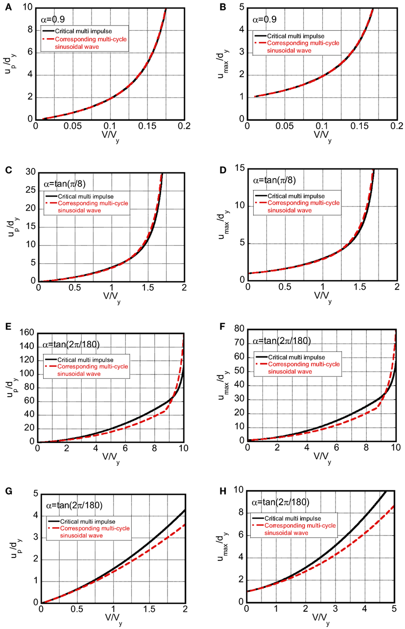
Figure 12. Comparison of plastic deformation and maximum deformation between critical multi impulse and corresponding multi-cycle sinusoidal wave: (A,B) α = 0.9, (C,D) α = tan(π/8) = 0.414, (E,F,G,H) α = tan(2π/180) = 0.0349 [(G,H) are magnified ones of (E,F)].

Proof of Critical Timing

In order to investigate the validity of the critical timing evaluated by Eq. 19a,b, the time-history response analysis has been conducted of the SDOF bilinear hysteresis system under the multi impulse with the varied impulse timing t₀ for various input velocity levels and various post-yield stiffness ratios. The critical timing of each impulse can be characterized as the time with zero restoring force as assumed in Section “Closed-Form Expression of Elastic–Plastic Steady-state Response under Critical Multi Impulse.” T₁ = 1.0 (s), d_y = 0.04 (m), Δt = 1.0 × 10⁻⁴T₁ are used in the time-history response analysis and the numbers of impulses used in the time-history response analysis for the convergence of the response are 1,000.

Figure 13 shows the normalized maximum deformation u_max/d_y and the normalized plastic deformation amplitude u_p/d_y with respect to the impulse timing $t_0/t_0^c$ normalized by the critical timing for various input velocity levels V/V_y and various post-yield stiffness ratios α = 0.035, 0.414, 0.9. It can be confirmed that the critical timing $t_0^c$ derived in Section “Derivation of Critical Impulse Timing” actually provides the critical case under the multi impulse and gives the upper bound of u_max/d_y and u_p/d_y. The closed-form expressions of u_max/d_y and u_p/d_y derived in Sections “Case 1: Impulse in Unloading Process” and “Case 2: Impulse in Loading Process (Second Stiffness Range)” are equal to the upper bound of u_max/d_y and u_p/d_y in Figure 13.

FIGURE 13

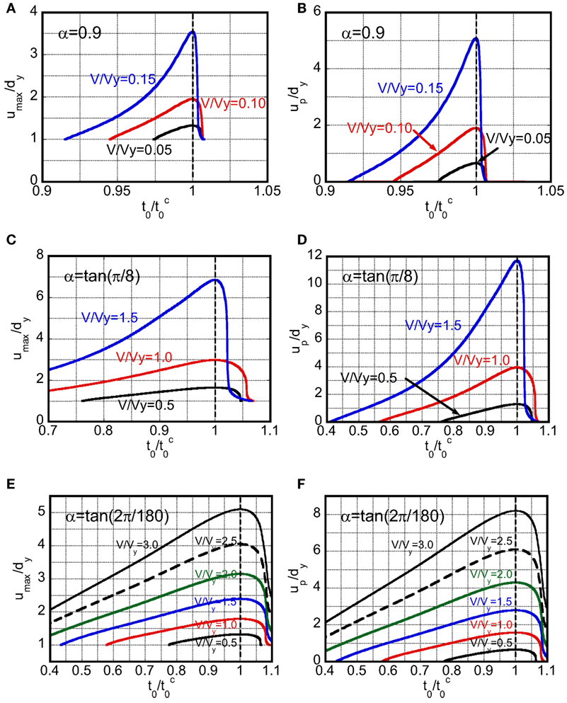
Figure 13. Maximum deformation and plastic deformation amplitude with respect to timing of multi impulse for various input levels: (A,B) α = 0.9, (C,D) α = tan(π/8) = 0.414, (E,F) α = tan(2π/180) = 0.0349.

Applicability of Critical Multi Impulse Timing to Corresponding Sinusoidal Wave

In Section “Accuracy Check by Time-History Response Analysis under the Corresponding Multi-Cycle Sinusoidal Wave,” it has been demonstrated that, if the maximum value of the Fourier amplitude is selected as a key parameter, the response under the multi impulse with the time interval obtained by Eq. 19a,b and that under the corresponding multi-cycle sinusoidal wave exhibit a fairly good correspondence. In this section, it is investigated whether the critical timing of the multi impulse derived in Section “Derivation of Critical Impulse Timing” is also an approximate critical period of the multi-cycle sinusoidal wave.

The resonant equivalent frequency of the harmonic wave for a specific acceleration amplitude has to be obtained by the resonance curve computed by using the exact solution (Iwan, 1961). In this procedure, it is necessary to solve the transcendental equation by changing the excitation frequency in a parametric manner. On the other hand, Caughey (1960a,b) has proposed the method to derive the equivalent resonance frequency directly by using the equivalent linearization method with the least squares approximation. However, this equivalent resonant frequency differs from the exact equivalent resonant frequency in the larger acceleration amplitude range. In these previous papers, the resonant equivalent frequency of the harmonic wave for a specific acceleration amplitude has been derived. However, the resonant equivalent frequency for a specific velocity amplitude has not been derived.

In order to calculate the maximum deformation and the plastic deformation amplitude under the corresponding multi-cycle sinusoidal wave with the varied period T_l for various input velocity levels and various post-yield stiffness ratios, the time-history response analysis has been conducted of the SDOF bilinear hysteresis system under the corresponding multi-cycle sinusoidal wave. T_l, ω_l = 2π/T_l, A_l, and V_l = A_l/ω_l denote the period, the circular frequency, the acceleration amplitude, and the velocity amplitude of the sinusoidal wave corresponding to the multi impulse with the equal time interval t₀ and the input velocity level V. In addition, T_l = 2t₀ is used in this section. The input period T_l is changed for the specific velocity amplitude calculated by Eq. 21 with the input velocity level V. ${T_l}^c=2t_0^c$ denotes the approximate critical period of the multi-cycle sinusoidal wave for a specific velocity amplitude V_l.

Figure 14 shows the normalized maximum deformation u_max/d_y and the normalized plastic deformation amplitude u_p/d_y with respect to the input period $T_l/{T_l}^c\left(=t_0/t_0^c\right)$ normalized by the approximate critical period for various input velocity levels V/V_y (corresponding to the velocity amplitude V_l) and various post-yield stiffness ratios α = 0.035, 0.414, 0.9. It can be observed that ${T_l}^c=2t_0^c$ is a fairly good approximate of the critical period of the multi-cycle sinusoidal wave for a specific velocity amplitude.

FIGURE 14

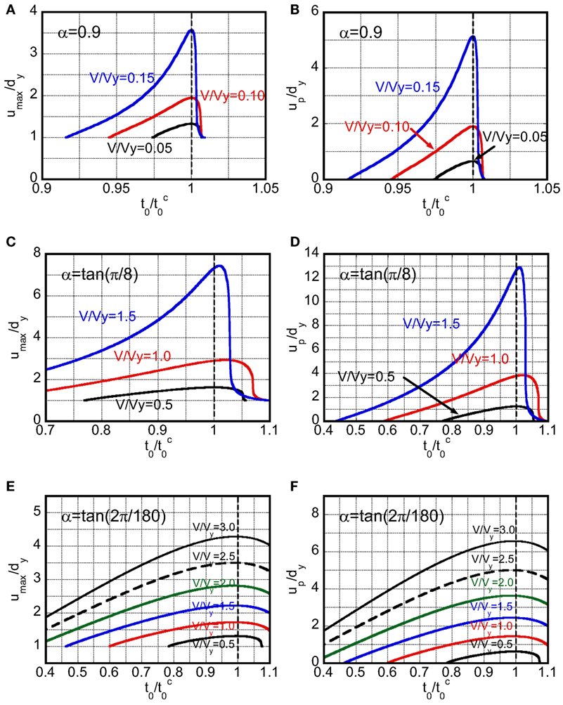
Figure 14. Maximum deformation and plastic deformation amplitude with respect to period of corresponding sinusoidal wave for various input levels: (A,B) α = 0.9, (C,D) α = tan(π/8) = 0.414, (E,F) α = tan(2π/180) = 0.0349.

Accuracy Check by Exact Solution Subjected to the Corresponding Multi-Cycle Sinusoidal Wave

The accuracy of the proposed closed-from steady-state response under the critical multi impulse is investigated through the comparison with the resonance curve under the corresponding sinusoidal wave computed by using the exact solution (Iwan, 1961). It is necessary for the resonance curve to solve the transcendental equation by changing the excitation frequency in a parametric manner and the resonant equivalent frequency of the harmonic wave for a specific acceleration amplitude has to be obtained by the resonance curve (Iwan, 1961). On the other hand, the proposed method provides directly the critical steady-state response for the specific input level by the closed-form expression. The input level of the multi impulse and the corresponding sinusoidal wave has been adjusted by using the equivalence of the maximum Fourier amplitude as explained in Sections “Accuracy Check by Time-History Response Analysis under the Corresponding Multi-Cycle Sinusoidal Wave” and “Applicability of Critical Multi Impulse Timing to Corresponding Sinusoidal Wave.”

Figure 15 shows the comparison of the proposed closed-form expression of the critical maximum deformation with respect to ω* with the resonance curve by Iwan (1961) [corresponding to Figures 11–13 in the study by Iwan (1961)]. ω* and r in Figure 15 denote the ratio of the excitation frequency ω_l = 2π/T_l of the corresponding sinusoidal wave to the elastic natural circular frequency ω₁ and the ratio of the excitation acceleration amplitude A_l = ω_lV_l of the corresponding sinusoidal wave to the parameter $A_y={\mathrm{\omega }}_1^2{d}_y$. r is also equal to the product of the mass m and the acceleration amplitude A_l normalized by the yield force f_y. The red line in Figure 15 shows the maximum deformation under the critical multi impulse. The normalized critical timing $t_0^c/T_1$ is converted to ${\mathrm{\omega }}^{\ast }=T_1/\left(2t_0^c\right)$ by using $T_l=2t_0^c$ in the critical case. The black line shows the resonance curve with r = 0.1 in Figure 15A, r = 0.3, 0.478, 0.746 in Figure 15B, r = 0.6, 0.955, 1.228 in Figure 15C. The black solid circles in Figure 15 present the resonance points for the specific acceleration amplitude. In addition, the blue dotted line in Figure 15 presents the resonance curve for constant velocity amplitude. It can be observed that the proposed closed-form expression of the critical maximum deformation under the multi impulse corresponds to the blue dotted line (constant velocity amplitude) better than the black line (constant acceleration amplitude).

FIGURE 15

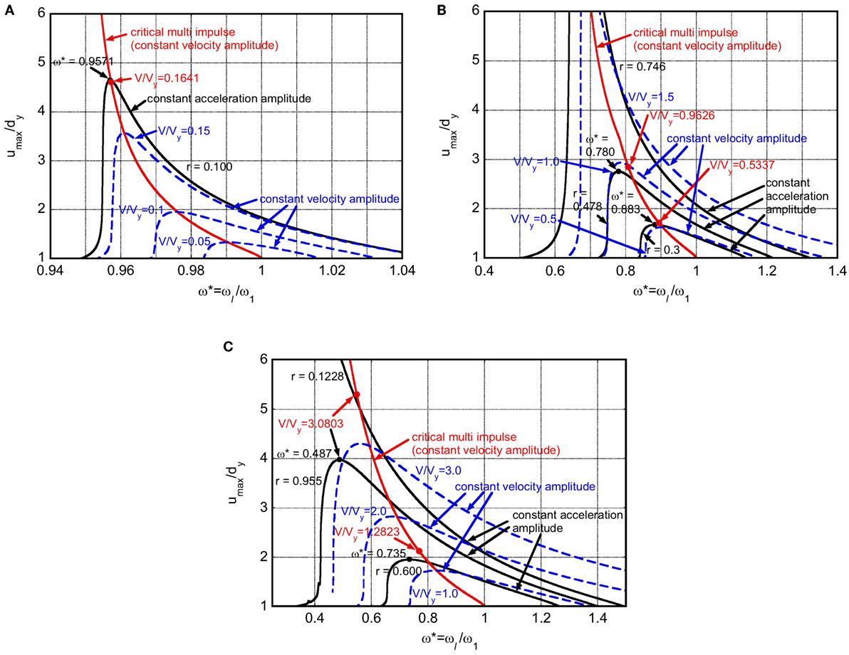
Figure 15. Comparison of closed-form maximum deformation under critical multi impulse (constant velocity amplitude) and resonance curve under sinusoidal wave (constant acceleration amplitude and constant velocity amplitude): (A) α = 0.9, (B) α = tan(π/8) = 0.414, (C) α = tan(2π/180) = 0.0349.

The red solid circles present the maximum deformation under the critical multi impulse for the input levels corresponding to the resonance points of the resonance curve (the black solid circles in Figure 15). The method to calculate the input velocity level corresponding to the resonant point (black solid circle) is explained next. From given parameters r, ω* (at the resonance point), and Eq. 21, the following relation can be obtained.

$V_l=A_l/{\mathrm{\omega }}_l=\left(r{\mathrm{\omega }}_1{V}_y\right)/\left({\mathrm{\omega }}^{\ast }{\mathrm{\omega }}_1\right)=\left(2/\mathrm{\pi }\right)V$ (22)

From Eq. 22, the normalized input velocity level can be obtained as follows:

$V/V_y=\left(\mathrm{\pi }/2\right)\left(r/{\mathrm{\omega }}^{\ast }\right)$ (23)

The maximum deformation u_max/d_y and the critical timing $t_0^c/T_1$ can be obtained by Eq. 5 or 16 and Eq. 19a or 19b depending on the input velocity level, respectively.

The results of the correspondence between the critical multi impulse and the critical sinusoidal wave are listed in Table 1. The responses and the resonant frequencies between the critical multi impulse and the critical sinusoidal wave exhibit fairly good correspondence except the case with α = tan(2π/180) and r = 0.600 (the small post-yield stiffness with the large input level).

TABLE 1

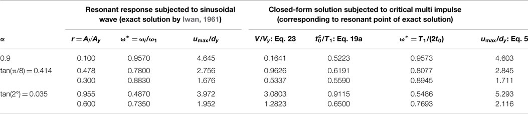
Table 1. Comparison of maximum deformations between sinusoidal wave and multi impulse.

Conclusion

The multi impulse has been introduced as a substitute of the long-duration ground motion and the closed-form expression has been derived of the steady-state elastic–plastic response of the SDOF bilinear hysteretic system under the critical multi impulse. While the resonant equivalent frequency of the elastic–plastic system for a specific input level has to be computed by changing the excitation frequency in a parametric manner in the conventional method dealing directly with the sinusoidal wave (Iwan, 1961), the steady-state elastic–plastic response under the critical multi impulse can be obtained in closed form (without repetition) and the critical time interval of the multi impulse (the resonant frequency) can also be obtained in closed form for the increasing input level in this proposed method. The following conclusions have been derived.

(1) The steady state in which the each impulse acts at the zero restoring-force point has been assumed and the closed-form expressions of the elastic–plastic response under the critical multi impulse have been derived by using the energy approach. The steady state under the critical multi impulse can be classified into two cases depending on the plastic deformation and the input velocity level. CASE 1 is the case where each impulse acts at the zero restoring-force timing in the unloading process and CASE 2 is the case where each impulse acts at the zero restoring-force timing in the loading process. The closed-form expressions of the critical time interval of the multi impulse in both CASE 1 and CASE 2 have been derived by solving the equations of motion and substituting the continuation conditions at the transition points.

(2) The response under the multi impulse with the equal time interval obtained in Section “Derivation of Critical Impulse Timing” converges into the steady state in which each impulse acts at the zero restoring force as shown in Figure 3. The maximum deformation and the plastic deformation amplitude after convergence into the steady state correspond to the closed-form expressions obtained in Section “Case 1: Impulse in Unloading Process” and Section “Case 2: Impulse in Loading Process (Second Stiffness Range).”

(3) The validity and accuracy of the proposed closed-form expressions have been investigated through the comparison with the steady-state response under the corresponding multi-cycle sinusoidal wave as a representative of the long-duration ground motion by using the time-history response analysis. It has been confirmed that the multi impulse provides a fairly good substitute of the multi-cycle sinusoidal wave in the evaluation of the maximum deformation and the plastic deformation amplitude if the maximum Fourier amplitude is adjusted.

(4) The validity of the critical time interval derived in Section “Derivation of Critical Impulse Timing” has been confirmed by using the time-history response analysis of the SDOF bilinear hysteresis system under the multi impulse with the varied impulse timing. The critical timing of each impulse can be characterized as the time with zero restoring force in the steady state.

(5) Twice the critical time interval is a good approximate of the critical period of the multi-cycle sinusoidal wave with the corresponding input amplitude.

In this paper, the closed-form expression of the critical elastic–plastic response has been derived for a specific input velocity level V of the multi impulse. The input velocity level V corresponds to the velocity amplitude of the long-duration ground motion. The earthquake ground motions have been recorded for 70–80 years all over the world and the most rational method in determining V is to predict the velocity amplitude and the period of the ground motion at a specific site from the magnitude and/or other parameters of the possible fault rupture. However, it seems quite difficult to predict a possible ground motion at a specific site even by the most advanced method. In such a situation, the most reliable method may be to determine the input velocity level V from the occurrence return period of ground motions and the level of importance of the object building structure. In this case, an allowable level of damage to the structure should be set depending on the level of importance of the structure. From an alternative view point, the following treatment may be possible. The relation between V/V_y and the ductility factor u_max/d_y has been obtained as a result of this paper. If two of V, V_y, u_max/d_y are given, the remaining one can be obtained. V_y represents the strength and stiffness parameter of the structure in velocity dimension. Therefore, if two among the structural parameter V_y (the strength and stiffness parameter of the structure), the input level V of the ground motion, the allowable damage level u_max/d_y of the structure are given, the remaining parameter can be determined. The final decision is entrusted to structural designers. It may be said that the present paper has offered a tool for such decision.

Author Contributions

KK carried out the theoretical and numerical analysis. IT supervised the theoretical formulation.

Conflict of Interest Statement

The authors declare that the research was conducted in the absence of any commercial or financial relationships that could be construed as a potential conflict of interest.

Funding

Part of the present work is supported by the Grant-in-Aid for Scientific Research (KAKENHI) of Japan Society for the Promotion of Science (No. 15H04079, 15J00960) and Sumitomo Rubber Industries, Co. This support is greatly appreciated.

References

Abrahamson, N., Ashford, S., Elgamal, A., Kramer, S., Seible, F., and Somerville, P. (1998). 1st PEER Workshop on Characterization of Special Source Effects. San Diego: Pacific Earthquake Engineering Research Center, University of California.

Google Scholar

Bertero, V. V., Mahin, S. A., and Herrera, R. A. (1978). Aseismic design implications of near-fault San Fernando earthquake records. Earthquake Eng. Struct. Dyn. 6, 31–42. doi:10.1002/eqe.4290060105

CrossRef Full Text | Google Scholar

Caughey, T. K. (1960a). Sinusoidal excitation of a system with bilinear hysteresis. J. Appl. Mech. 27, 640–643. doi:10.1115/1.3644077

CrossRef Full Text | Google Scholar

Caughey, T. K. (1960b). Random excitation of a system with bilinear hysteresis. J. Appl. Mech. 27, 649–652. doi:10.1115/1.3644077

CrossRef Full Text | Google Scholar

Iwan, W. D. (1961). The Dynamic Response of Bilinear Hysteretic Systems. Ph.D. thesis, California Institute of Technology, Pasadena.

Google Scholar

Iwan, W. D. (1965a). “The dynamic response of the one-degree-of-freedom bilinear hysteretic system,” in Proc. of the Third World Conf. on Earthquake Eng (New Zealand).

Google Scholar

Iwan, W. D. (1965b). The steady-state response of a two-degree-of- freedom bilinear hysteretic system. J. Appl. Mech. 32, 151–156. doi:10.1115/1.3625711

CrossRef Full Text | Google Scholar

Kalkan, E., and Kunnath, S. K. (2006). Effects of fling step and forward directivity on seismic response of buildings. Earthquake Spectra 22, 367–390. doi:10.1193/1.2192560

CrossRef Full Text | Google Scholar

Kojima, K., and Takewaki, I. (2015a). Critical earthquake response of elastic-plastic structures under near-fault ground motions (Part 1: fling-step input). Front. Built Environ. 1:12. doi:10.3389/fbuil.2015.00012

CrossRef Full Text | Google Scholar

Kojima, K., and Takewaki, I. (2015b). Critical earthquake response of elastic-plastic structures under near-fault ground motions (Part 2: forward-directivity input). Front. Built Environ. 1:13. doi:10.3389/fbuil.2015.00013

CrossRef Full Text | Google Scholar

Kojima, K., and Takewaki, I. (2015c). Critical input and response of elastic-plastic structures under long-duration earthquake ground motions. Front. Built Environ. 1:15. doi:10.3389/fbuil.2015.00015

CrossRef Full Text | Google Scholar

Kojima, K., and Takewaki, I. (2016). Closed-form critical earthquake response of elastic-plastic structures with bilinear hysteresis under near-fault ground motions. J. Struct. Constr. Eng. 726, 1209–1219. doi:10.3130/aijs.81.1209

CrossRef Full Text | Google Scholar

Liu, C.-S. (2000). The steady loops of SDOF perfectly elastoplastic structures under sinusoidal loadings. J. Mar. Sci. Technol. 8, 50–60.

Google Scholar

Roberts, J. B., and Spanos, P. D. (1990). Random Vibration and Statistical Linearization. New York, NY: Wiley.

Google Scholar

Takewaki, I., Murakami, S., Fujita, K., Yoshitomi, S., and Tsuji, M. (2011). The 2011 off the Pacific coast of Tohoku earthquake and response of high-rise buildings under long-period ground motions. Soil Dyn. Earthquake Eng. 31, 1511–1528. doi:10.1016/j.soildyn.2011.06.001

CrossRef Full Text | Google Scholar

Appendix 1

Time-History Response under Critical Multi Impulse and Derivation of Critical Time Interval

The closed-form expressions of the time-history response under the critical multi impulse and the critical time interval in the steady state are derived by solving the equation of motion directly.

First of all, the time-history response for CASE 1 is derived. Figures 4B,C show the time histories of the deformation and the restoring force in CASE 1. By solving the equation of motion in the path between point F and B in Figure 4A and substituting the displacement and velocity conditions at point A, the time-history response after the impulse acting point (point A in Figure 4A) can be expressed as follows:

$u\left(t\right)=\mathrm{\{}\left(v_c+V\right)/V_y\mathrm{\}}{d}_y\text{sin}\left({\mathrm{\omega }}_{1}t\right)-0.5\left(1-\mathrm{\alpha }\right)u_p$ (A1a)

$\dot{u}\left(t\right)=\left(v_c+V\right)\text{cos}\left({\mathrm{\omega }}_{1}t\right)$ (A1b)

In Eqs A1a and A1b, t = 0 is set at point A and v_c, u_p can be obtained from Eqs 2 and 4. The time interval between point A and B in Figure 4 is denoted by t_AB as shown in Figures 4B,C. t_AB can then be obtained as follows from u(t = t_AB) = d_y − 0.5u_p and Eq. A1a.

$t_{\mathit{AB}}/T_1=\mathrm{\{}1/\left(\mathrm{2\pi }\right)\mathrm{\}}\arcsin \left[\mathrm{\{}1-0.\mathrm{5\alpha }\left(u_p/d_y\right)\mathrm{\}}/\mathrm{\{}\left(v_c+V\right)/V_y\mathrm{\}}\right]$ (A2)

The time-history response after the yielding point (point B in Figure 4) can be expressed as follows:

$u\left(t\right)=\left(\frac{1}{\mathrm{\alpha }}-0.5\frac{u_p}{d_y}\right)d_y\text{cos}\left(\sqrt{\mathrm{\alpha }}{\mathrm{\omega }}_{1}t\right)+\frac{1}{\sqrt{\mathrm{\alpha }}}\frac{v_B}{V_y}{d}_y\text{sin}\left(\sqrt{\mathrm{\alpha }}{\mathrm{\omega }}_{1}t\right)-\left(\frac{1}{\mathrm{\alpha }}-1\right)d_y$ (A3a)

$\dot{u}\left(t\right)=-\sqrt{\mathrm{\alpha }{\left(\frac{1}{\mathrm{\alpha }}-0.5\frac{u_p}{d_y}\right)}^2+{\left(\frac{v_B}{V_y}\right)}^2}{V}_y\times \text{sin}\left[\sqrt{\mathrm{\alpha }}{\mathrm{\omega }}_{1}t-\arctan \frac{v_B/V_y}{\sqrt{\mathrm{\alpha }}\mathrm{\{}\left(1/\mathrm{\alpha }\right)-0.5\left(u_p/d_y\right)\mathrm{\}}}\right]$ (A3b)

In Eqs A3a and A3b, t = 0 at point B and the velocity v_B at point B can be obtained as shown in Eq. 20 by the following energy balance law between point A and point B.

$m{\left(v_c+V\right)}^2/2=\left(m{v}_B^2/2\right)+\mathrm{\{}{\left(f_y-0.\mathrm{5\alpha }k{u}_p\right)}^2/2k\mathrm{\}}$ (A4)

The time interval between point B and C in Figure 4 is denoted by t_BC as shown in Figures 4B,C. t_BC can then be obtained as follows from $\dot{u}\left(t=t_{\mathit{BC}}\right)=0$ and Eq. A3b.

$t_{\mathit{BC}}/T_1=\mathrm{\{}1/\left(\mathrm{2\pi }\sqrt{\mathrm{\alpha }}\right)\mathrm{\}}\arctan \left[\frac{v_B/V_y}{\sqrt{\mathrm{\alpha }}\mathrm{\{}\left(1/\mathrm{\alpha }\right)-0.5\left(u_p/d_y\right)\mathrm{\}}}\right]$ (A5)

The time-history response after the unloading initiation point (point C in Figure 4) can be expressed as follows:

$u\left(t\right)=\mathrm{\{}1+0.\mathrm{5\alpha }\left(u_p/d_y\right)\mathrm{\}}{d}_y\text{cos}\left({\mathrm{\omega }}_{1}t\right)+0.5\left(1-\mathrm{\alpha }\right)u_p$ (A6a)

$\dot{u}\left(t\right)=-\mathrm{\{}1+0.\mathrm{5\alpha }\left(u_p/d_y\right)\mathrm{\}}{V}_y\text{sin}\left({\mathrm{\omega }}_{1}t\right)$ (A6b)

In Eqs A6a and A6b, t = 0 is set at point C. The time interval between point C and D in Figure 4 is denoted by t_CD as shown in Figures 4B,C. t_CD can be then obtained as follows from u(t = t_CD) = 0.5(1 − α)u_p and Eq. A6a.

$t_{\mathit{CD}}/T_1=0.25$ (A7)

From Eqs. A2, A5, and A7 and Figures 4B,C, the time interval $t_0^c$ between two consecutive impulses acting at the zero restoring-force points (points A and D) in CASE 1 can be obtained as follows:

$\begin{array}{l}{t}_0^c/T_1=\left(t_{\mathit{AB}}/T_1\right)+\left(t_{\mathit{BC}}/T_1\right)+\left(t_{\mathit{CD}}/T_1\right)\hfill \\ =\frac{1}{\mathrm{2\pi }}\left[\arcsin \left\{\frac{1-0.\mathrm{5\alpha }\left(u_p/d_y\right)}{\left(v_c+V\right)/V_y}\right\}+\frac{1}{\sqrt{\mathrm{\alpha }}}\arctan \left\{\frac{1}{\sqrt{\mathrm{\alpha }}}\frac{v_B/V_y}{\left(1/\mathrm{\alpha }\right)-0.5\left(u_p/d_y\right)}\right\}\right]+\frac{1}{4}\hfill \\ \text{for }V/V_y\le -2+2\sqrt{1/\mathrm{\alpha }}\hfill \end{array}$ (A8)

Second, the time-history response for CASE 2 is derived. Figures 6B,C show the time histories of the deformation and the restoring force in CASE 2. The time-history response after the impulse acting point (point A in Figure 6) can be expressed as follows:

$u\left(t\right)=\mathrm{\{}\left(v_c+V\right)/\left(\sqrt{\mathrm{\alpha }}{V}_y\right)\mathrm{\}}{d}_y\text{sin}\left(\sqrt{\mathrm{\alpha }}{\mathrm{\omega }}_{1}t\right)-\mathrm{\{}\left(1/\mathrm{\alpha }\right)-1\mathrm{\}}{d}_y$ (A9a)

$\dot{u}\left(t\right)=\left(v_c+V\right)\text{cos}\left(\sqrt{\mathrm{\alpha }}{\mathrm{\omega }}_{1}t\right)$ (A9b)

In Eqs A9a and A9b, t = 0 is set at point A and v_c, u_p can be obtained from Eqs 13 and 15. The time interval between point A and B in Figure 6 is denoted by t_AB as shown in Figures 6B,C. t_AB can be then obtained as follows from $\dot{u}\left(t=t_{\mathit{AB}}\right)=0$ and Eq. A9b.

$t_{\mathit{AB}}/T_1=\mathrm{\{}1/\left(\mathrm{2\pi }\right)\mathrm{\}}\mathrm{\{}\mathrm{\pi }/\left(2\sqrt{\mathrm{\alpha }}\right)\mathrm{\}}=1/\left(4\sqrt{\mathrm{\alpha }}\right)$ (A10)

The time-history response after the unloading initiation point (point B in Figure 6) can be expressed as follows:

$u\left(t\right)=\mathrm{\{}1+0.\mathrm{5\alpha }\left(u_p/d_y\right)\mathrm{\}}{d}_y\text{cos}\left({\mathrm{\omega }}_{1}t\right)+\left(1-\mathrm{\alpha }\right)0.5u_p$ (A11a)

$\dot{u}\left(t\right)=-\mathrm{\{}1+0.\mathrm{5\alpha }\left(u_p/d_y\right)\mathrm{\}}{V}_y\text{sin}\left({\mathrm{\omega }}_{1}t\right)$ (A11b)

In Eqs A11a and A11b, t = 0 is set at point B. The time interval between point B and C in Figure 6 is denoted by t_BC as shown in Figures 6B,C. t_BC can then be obtained as follows from u(t = t_BC) = − d_y + 0.5u_p and Eq. A11a.

$t_{\mathit{BC}}/T_1=\left(1/4\right)-\mathrm{\{}1/\left(\mathrm{2\pi }\right)\mathrm{\}}\arcsin \left[\frac{0.\mathrm{5\alpha }\left(u_p/d_y\right)-1}{0.\mathrm{5\alpha }\left(u_p/d_y\right)+1}\right]$ (A12)

The time-history response after the yielding initiation point (point C in Figure 6) can be expressed as follows:

$u\left(t\right)=-\sqrt{{\left(-\frac{1}{\mathrm{\alpha }}+0.5\frac{u_p}{d_y}\right)}^2+\left(2\frac{u_p}{d_y}\right)}{d}_y\times \text{sin}\left\{\sqrt{\mathrm{\alpha }}{\mathrm{\omega }}_{1}t-\arctan \frac{0.5\left(u_p/d_y\right)-\left(1/\mathrm{\alpha }\right)}{\sqrt{2u_p/d_y}}\right\}+\left(\frac{1}{\mathrm{\alpha }}-1\right)d_y$ (A13a)

$\dot{u}\left(t\right)=-\sqrt{\mathrm{\alpha }\left\{{\left(-\frac{1}{\mathrm{\alpha }}+0.5\frac{u_p}{d_y}\right)}^2+\left(2\frac{u_p}{d_y}\right)\right\}}{V}_y\times \text{cos}\left\{\sqrt{\mathrm{\alpha }}{\mathrm{\omega }}_{1}t-\arctan \frac{0.5\left(u_p/d_y\right)-\left(1/\mathrm{\alpha }\right)}{\sqrt{2u_p/d_y}}\right\}$ (A13b)

In Eqs A13a and A13b, t = 0 is set at point C. The time interval between point C and D in Figure 6 is denoted by t_CD as shown in Figures 6B,C. t_CD can then be obtained as follows from u(t = t_CD) = {(1/α) − 1}d_y and Eq. A13a.

$t_{\mathit{CD}}/T_1=\frac{1}{\sqrt{\mathrm{\alpha }}}\frac{1}{\mathrm{2\pi }}\arctan \left\{\frac{0.5\left(u_p/d_y\right)-\left(1/\mathrm{\alpha }\right)}{\sqrt{2\left(u_p/d_y\right)}}\right\}$ (A14)

From Eqs A10, A12, and A14 and Figures 6B,C, the time interval $t_0^c$ between two consecutive impulses acting at the zero restoring-force points (points A and D) in CASE 2 can then be obtained as follows:

$\begin{array}{l}{t}_0^c/T_1=\left(t_{\mathit{AB}}/T_1\right)+\left(t_{\mathit{BC}}/T_1\right)+\left(t_{\mathit{CD}}/T_1\right)\hfill \\ =\frac{1}{4}\left(1+\frac{1}{\sqrt{\mathrm{\alpha }}}\right)+\frac{1}{\mathrm{2\pi }}\left[-\arcsin \left\{\frac{0.\mathrm{5\alpha }\left(u_p/d_y\right)-1}{0.\mathrm{5\alpha }\left(u_p/d_y\right)+1}\right\}+\frac{1}{\sqrt{\mathrm{\alpha }}}\arctan \left\{\frac{0.5\left(u_p/d_y\right)-\left(1/\mathrm{\alpha }\right)}{\sqrt{2\left(u_p/d_y\right)}}\right\}\right]\hfill \\ \text{for }V/V_y>-2+2\sqrt{1/\mathrm{\alpha }}\end{array}$ (A15)

Appendix 2

Adjustment of Input Level of Multi Impulse and Corresponding Sinusoidal Wave

The adjustment method of input level of the multi impulse and the corresponding sinusoidal wave is explained based on the equivalence of the maximum Fourier amplitude.

Consider the multi impulse as a representative of a long-duration ground acceleration as shown in Figure 2A, expressed by

${ü}_g\left(t\right)=V\mathrm{\delta }\left(t\right)-V\mathrm{\delta }\left(t-t_0\right)+V\mathrm{\delta }\left(t-2t_0\right)-V\mathrm{\delta }\left(t-3t_0\right)+\cdots +{\left(-1\right)}^{N-1}V\mathrm{\delta }\mathrm{\{}t-\left(N-1\right)t_0\mathrm{\}}$ (A16)

where N is the number of impulses. The corresponding multi-cycle sinusoidal wave ${{ü}_g}^{\text{SW}}\left(t\right)$ is expressed as follows:

${ü}_g^{\text{SW}}\left(t\right)=A_l\text{sin}\left({\mathrm{\omega }}_{l}t\right)\left(0\le t\le 0.5N{T}_l=N{t}_0\right)$ (A17)

where A_l is the acceleration amplitude, T_l = 2t₀ is the excitation period, ω_l = 2π/T_l is the excitation circular frequency and V_l = A_l/ω_l is the velocity amplitude. The number of cycles is half of the number of impulses.

The maximum Fourier amplitude of the multi impulse ${ü}_g\left(t\right)$ and that of the corresponding multi-cycle sinusoidal wave ${ü}_g^{\text{SW}}\left(t\right)$ can be derived as follows:

$\text{max}\mathrm{|}{Ü}_g\left(\mathrm{\omega }\right)\mathrm{|}=V\left\{\text{max}\left|{\sum }_{n=0}^{N-1}{\left(-1\right)}^n{e}^{-i\mathrm{\omega }n{t}_0}\right|\right\}=\mathit{NV}$ (A18)

$\text{max}\mathrm{|}{Ü}_g^{\text{SW}}\left(\mathrm{\omega }\right)\mathrm{|}=A_l\left\{\text{max}\left|\frac{\mathrm{2\pi }{t}_0}{{\mathrm{\pi }}^2-{\left(\mathrm{\omega }{t}_0\right)}^2}\text{sin}\left(0.5N\mathrm{\omega }{t}_0\right)\right|\right\}$ (A19)

The function $f\left(\mathrm{\omega }{t}_0\right)=\mathrm{2\pi }{t}_0\mathrm{|}\text{sin}\left(0.5N\mathrm{\omega }{t}_0\right)/\mathrm{\{}{\mathrm{\pi }}^2-{\left(\mathrm{\omega }{t}_0\right)}^2\mathrm{\}}\mathrm{|}$ can be defined from Eq. A19. If N is a sufficiently large number of impulses (e.g., over 20 impulses), the function f (x = ωt₀) is maximized at ωt₀ = π and the maximum value of f(x = ωt₀) can be obtained as follows by using l’Hospital’s theorem.

$\underset{\mathrm{\omega }{t}_0\to \mathrm{\pi }}{\lim }\left|\frac{\text{sin}\left(0.5N\mathrm{\omega }{t}_0\right)}{{\mathrm{\pi }}^2-{\left(\mathrm{\omega }{t}_0\right)}^2}\right|=\underset{\mathrm{\omega }{t}_0\to \mathrm{\pi }}{\lim }\left|\frac{0.5N\text{cos}\left(0.5N\mathrm{\omega }{t}_0\right)}{-2\left(\mathrm{\omega }{t}_0\right)}\right|=\frac{N}{\mathrm{4\pi }}$ (A20)

N is assumed here to be an even number. From Eqs A18, A19, and A20, the following relation can be obtained by using the equivalence $\text{max}\mathrm{|}{Ü}_g\left(\mathrm{\omega }\right)\mathrm{|}=\text{max}\mathrm{|}{Ü}_g^{\text{SW}}\left(\mathrm{\omega }\right)\mathrm{|}$ of the maximum Fourier amplitude.

$V_l=A_l/{\mathrm{\omega }}_l=\left(2/\mathrm{\pi }\right)V$ (A21)