Data-Interpretation Methodologies for Non-Linear Earthquake Response Predictions of Damaged Structures

Introduction

Earthquakes still pose a major threat to the integrity of existing buildings. Although significant progress has been made on earthquake-resistant design methodologies, large parts of the building stock continue to sustain damage from earthquake actions. Structural damage to buildings after an earthquake is inevitable, especially in the context of design specifications being generally limited to the protection of building occupants rather than guaranteeing structural integrity in regions with low to medium earthquake hazard (Priestley, 2000). In addition, regions with low to medium seismicity are often characterized by large amounts of buildings that have been designed without consideration of the seismic limit state.

Current practice for building assessment after earthquakes exclusively relies on visual inspection. However, large numbers of buildings need inspection in such a context. Combined with a potential need for multiple inspections of the same buildings, important economic losses can result from restricted access leading to loss of business opportunities and needs for provisional housing. Also, visual inspection has been shown to produce subjective assessment results (Marshall et al., 2013; Galloway et al., 2014).

Evaluation of increased vulnerability during aftershocks of buildings damaged by mainshocks of an earthquake sequence is a known challenge, and it has recently received attention in risk assessment during the design stage (Nazari et al., 2015). In addition, updated vulnerability assessments for buildings characterized by a given damage state after a mainshock have been proposed (Réveillère et al., 2012; Jeon et al., 2015; Raghunandan et al., 2015). Jalayer et al. (2011) proposed an updating approach for aftershock probabilities to enhance post-earthquake reliability assessment using single-degree-of-freedom models. However, few studies incorporate measurement interpretation to update vulnerability curves after the main shock. In addition, uncertainties are generally limited to ground motion parameters, not behavior modeling uncertainties.

Measurement-based structural identification has the potential to improve upon current assessment techniques and to complement visual inspection. Measurement data can, thus, provide an objective support for post-earthquake decision-making. In addition, identifying parameters of physical models allows engineers to predict structural behavior during future earthquakes and can support the design of retrofitting and strengthening.

Ambient vibrations are an attractive data source in a post-earthquake context as small, sensitive and affordable sensors have emerged. Ambient vibrations are non-destructive and can be measured without any form of actuation and, therefore, ambient vibration measurements are potentially cost-effective and time-efficient. However, a well-known drawback of ambient vibration measurements is the very low amplitude of excitation, resulting in mostly linear responses. In addition, despite controversial results, modal properties derived from ambient vibrations have been shown in the past to be potential indicators of structural damage (Mucciarelli et al., 2004; Clinton et al., 2006; Michel et al., 2011). As a consequence, many proposals for structural identification based on vibrations measurements for damage detection have emerged (Chellini et al., 2010; Moaveni et al., 2010; Behmanesh et al., 2017).

Structural identification based on Bayes’ theorem to identify hysteretic models has been proposed (Muto and Beck, 2008; Worden and Hensman, 2012; Green and Worden, 2015). However, predicting non-linear behavior with models that have been identified using exclusively linear measurements involves extrapolation. As structural models are a simplified and approximate representation of real structures, model error, defined as the discrepancy between model predictions and observed behavior, cannot be avoided. Such model error is epistemic and systematic, meaning model error is often spatially correlated. The challenge of this type of error for inverse engineering tasks, such as structural identification, has been discussed (Tarantola, 2006; Fernández-Martínez et al., 2013; Brynjarsdóttir and O’Hagan, 2014). However, in a scenario that involves extrapolation, such as predicting non-linear displacement demands with models that are identified using natural frequencies, the model uncertainty differs from identification to prediction. Few studies have been found to assess accuracy and precision of identified non-linear structural models identified based on linear measurements with respect to prediction intervals for non-linear extrapolations. As single answers are ill-suited for such inverse problems, prediction ranges involving bounds on uncertainty are needed and proposed in this paper.

Asgarieh et al. (2017) assessed the influence of model error on the calibration of non-linear parameters of a structural model. However, no comparative study of identification methodologies was proposed for identification of non-linear models with linear measurements. In addition, the consequences of erroneous uncertainty definition were not evaluated.

In this paper, three structural identification methodologies are compared. The background and underlying assumptions related to Bayesian model updating (BMU) involving traditional and modified likelihood function formulations as well as error-domain model falsification (EDMF) methodologies are described and compared. A methodology to derive non-linear structural parameters from linear modal structural properties is provided. These three structural identification methodologies are then applied to a numerical case study and the robustness and precision regarding parameter identification and behavior extrapolation are compared.

Background

Error-domain model falsification, traditional Bayesian model updating (TBMU), and modified Bayesian model updating (MBMU) are compared. These three methodologies result in populations of solution through taking uncertainties into account. However, the methodologies differ in their initial formulation, starting points, assumptions related to the sources and forms of uncertainty, as well as the implementation of uncertainties.

Error-Domain Model Falsification

Error-domain model falsification implements a model falsification strategy that is based on the principles of scientific discovery (Popper, 1959). Rather than validating or optimizing single models, measurement data should ideally be used to falsify inappropriate model instances (Robert-Nicoud et al., 2005). The applicability of model falsification provides robust solutions to inverse engineering problems that are complicated by significant amounts of measurement and model uncertainty (Tarantola, 2006; Fernández-Martínez et al., 2013), particularly in the presence of model bias (Pasquier and Smith, 2015a).

A population of model instances is created through discrete samples of parameter combinations and, subsequently, used to simulate structural behavior (Raphael and Smith, 1998). The concept of simulating discrete populations of parameter combinations and discarding models that fail to predict measured behavior according to probabilistic criteria has been formalized by Goulet and Smith (2013) to develop a structural identification methodology called EDMF.

Error-domain model falsification explicitly takes into account measurement and modeling uncertainties resulting from multiple sources that are estimated to be biased (Goulet et al., 2013). Residuals between measured and predicted behavior are compared to thresholds for each measured quantity. Therefore, the acceptance region in the error-domain or residual-domain is a hypercube, which results in a model identification process that is usually insensitive to wrong correlation estimates. Correlations between uncertainties related to various measurements cannot be known precisely, therefore, prediction accuracy is sacrificed in EDMF in order to improve the robustness of prediction ranges. Also, EDMF results in uniform probabilities of candidate models, rather than more detailed probability distributions, thus reflecting the lack of knowledge of uncertainty forms in practical situations. Reduced sensitivity to uncertainty correlations and uniform prediction distributions increase robustness especially for prediction tasks, where behavior is predicted for conditions that differ from the measured configuration (Pasquier and Smith, 2015a). Extrapolation is required for decision-making in asset management for activities, such as repair, extension, and increasing service-life.

Tens of full-scale applications in several countries have confirmed that EDMF is intuitively understood by practicing engineers who need to interpret measurement data and field observations (Smith, 2016). This aspect is important for iterative data-interpretation tasks when information becomes available gradually over long periods. In such situations, specialized consultants cannot provide complete support. Engineers who are responsible for assets need to be able to comprehend how data are interpreted so that iterations following changes and discovery of new information can be carried out.

Error-domain model falsification, like any model-based structural identification methodology, relies on the comparison of predictions of model instances with measurements. Intervals of possible parameter values are defined for the parameters θ = {θ₁,…,θ_n} of a physics-based model g(.) through engineering heuristics and past experience. The parameter space is then sampled in order to obtain a discrete initial population of model instances. Applications of EDMF rely on grid sampling, Latin hypercube sampling and stochastic search to sample the parameter space (Robert-Nicoud et al., 2005; Goulet et al., 2010; Pasquier et al., 2014; Pasquier and Smith, 2015a).

For all n_m measured quantities the predictions of the physics-based model, g_i(θ), are compared to the measurement, y_i. Measurement data are conditioned by measurement error, ε_y. In addition, physics-based models are simplified and idealized representations of complex open-world structures. Therefore, the model prediction, g(θ), is conditioned by a significant model error, ε_g. For full-scale applications, model errors have been observed to be an order of magnitude higher than measurement error and are likely to be biased (Pasquier and Smith, 2015b).

When error estimates, ε_y and ε_g, are accurate, the true parameter values, θ*, can be obtained through Eq. 1.

$g_i\left({\mathrm{\theta }}^{\ast }\right)+{\mathrm{\epsilon }}_g=y_i+{\mathrm{\epsilon }}_y$ (1)

However, in open-world applications, modeling error and measurement error cannot be estimated deterministically. Nevertheless, conservative estimates of the uncertainty resulting from model and measurement error can be established through engineering knowledge. Generally, such heuristic estimates of model uncertainties, U_g, and measurement uncertainties, U_y, take the form of bounded intervals. If there is additional information regarding some uncertainty distributions, more elaborate distributions can be used.

A joint probability density function (PDF), f_Ui(u), of the total uncertainty f_U is obtained by combining measurement and modeling uncertainties. The total uncertainty f_U reflects the engineering estimate of acceptable levels of error on the residual between measurement data and model predictions. Therefore, thresholds are derived from the uncertainty to falsify inappropriate models.

In order to calculate the thresholds, a target identification probability ϕ_d is fixed. The probability of false rejection of the correct parameter combination is, thus, given by (1-ϕ_d) for correctly estimated uncertainty distributions. The thresholds, T_low,i and T_high,i, delimitate the shortest interval that has a cumulative probability equal to the fixed target probability as shown in Eq. 2. Residuals are compared to thresholds for all the n_m measured quantities, therefore, the Šidák correction for multiple hypothesis testing is applied to the target probability (Šidák, 1967), see Eq. 2.

${{\mathrm{\varphi }}_d}^{1∕n_m}={\int }_{T_{\text{low,}i}}^{T_{\text{high,}i}}{f}_{U_i}\left(u\right)\mathit{du}$ (2)

The candidate model set (CMS) is defined by all parameter combination instances of the initial model population that verify Eq. 3 for all nm measured and predicted quantities.

$\forall i\in \left\{1,\dots ,n_m\right\}:T_{\text{low,}i}\le g\left(\mathrm{\theta }\right)-y_i\le T_{\text{high,}i}$ (3)

The complete CMS is used to perform behavior predictions. When structural behavior, q_i, is predicted, the model uncertainty is added to the prediction range to comply with Eq. 1, as shown in Eq. 4. For interpolation tasks, the model uncertainty U_g equals the model error used for identification. If extrapolation is performed, the model uncertainty needs to be re-evaluated.

$q_i=g_i\left(\mathrm{\theta }\right)+U_g$ (4)

Traditional Bayesian Model Updating

Traditional Bayesian model updating is based on the Bayes theorem of conditional probability. Multiple applications of BMU have been proposed in the past for static and dynamic measurement data (Beck and Katafygiotis, 1998; Vanik et al., 2000; Katafygiotis and Yuen, 2001; Cheung and Beck, 2009; Lam et al., 2017; Marsili et al., 2017).

Based on the Bayes theorem of conditional probability, prior knowledge of model parameters θ is updated using a vector of measurement data y. The inference of an updated (or posterior) PDF p(θ|y) is calculated using a likelihood function p(y|θ) according to Eq. 5 that is based on Bayes’ conditional probability.

$p\left(\mathrm{\theta }|\mathit{\text{y}}\right)=\frac{p\left(y|\mathrm{\theta }\right)p\left(\mathrm{\theta }\right)}{p\left(y\right)}$ (5)

Traditional applications of BMU, also referred to as Bayesian inference, use zero-mean normal (or Gaussian) PDF formulations as likelihood function (see Eq. 6).

$p\left(\mathit{\text{y}}|\mathrm{\theta }\right)\propto \text{exp}\left[-\frac{{\left(\mathit{\text{y}}-\mathit{\text{g}}\left(\mathrm{\theta }\right)\right)}^{\prime }{\Sigma }^{-1}\left(\mathit{\text{y}}-\mathit{\text{g}}\left(\mathrm{\theta }\right)\right)}{2}\right]$ (6)

Most often, the covariance matrix $\Sigma \mathrm{ϵ}{\mathbb{R}}^{n_m\times n_m}$ that defines the likelihood function and that is composed of the variances and co-variances for each measurement is simplified. A recurrent assumption is independence between measurements that results in all non-diagonal terms equaling 0, according to the principle of maximum entropy (Simoen et al., 2013; Ebrahimian et al., 2017). A widespread technique is to parametrize the diagonal terms ${\mathrm{\sigma }}_i^2$, in order to estimate the likelihood function using available measurement data. In absence of modeling errors, such likelihood functions may be adequate estimations of the total uncertainty (Behmanesh et al., 2015).

The parameter space is sampled using Markov-chain Monte-Carlo (MCMC) sampling (Papadimitriou et al., 1997; Beck and Au, 2002), for which the sampling is guided using the likelihood function.

Modified Bayesian Model Updating

Modified Bayesian model updating is a novel formulation of BMU that avoids relying on zero-mean Gaussian likelihood functions. Relying on likelihood functions that are non-informed (constant probability) distributions is the most obvious difference between TBMU and MBMU. In environmental engineering, relying on uniform likelihood functions is sometimes referred to as generalized likelihood uncertainty estimation (Beven and Binley, 1992; Stedinger et al., 2008). By relying on a L∞-norm PDF (see Eq. 7), the likelihood function takes the form of bounds. In a similar way to EDMF, a likelihood function that takes the form of bounds is robust with respect to unknown and evolving correlations between measured quantities (Pai and Smith, 2017). Also, MBMU corrects for the number of measurements through applying the Šidák correction in a similar way to EDMF. MCMC sampling schemes are used similar to TBMU.

$p\left(\mathit{\text{y}}|\mathrm{\theta },\mathrm{\kappa }\right)\propto \text{exp}\left[-\left(\frac{1}{\mathrm{\kappa }}\right){\left|\frac{\left(\mathit{\text{y}}-\mathit{\text{g}}\left(\mathrm{\theta }\right)\right)-\mathrm{\mu }}{I^t\Sigma \text{I}}\right|}^{\mathrm{\kappa }}\right]$ (7)

Structural Identification with Non-Linear Models Based on Modal Properties

For structures that show non-linear behavior and where ultimate limit states need to be assessed, non-linear structural identification is needed. However, non-linear structural identification of buildings is complicated by the fact that non-destructive tests are limited to the linear range of structural behavior. Unless time-histories are measured during extreme events, such as earthquakes, no measurement data in the non-linear range are available. Therefore, in this paper, modal properties that characterize the linear behavior before and after an earthquake are used to identify parameters of a non-linear behavior model. Hysteretic non-linear time-series simulations are applied to link the building state before and after an earthquake (see Figure 1).

FIGURE 1

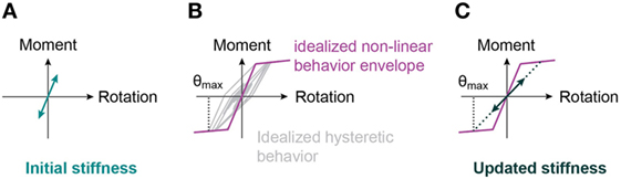
Figure 1. Updated stiffness for a moment-resisting spring undergoing hysteretic non-linear moment-rotation cycles. (A) Initial state, (B) earthquake, and (C) damaged state.

Simulation of non-linear time-series requires knowledge of the ground motion parameters that characterized the earthquake. If such knowledge is unavailable due to a coarse seismological network, multiple earthquakes need to be simulated in order to reflect the uniqueness and spatial variability of earthquake signals.

Error-domain model falsification as well as BMU involves multiple model simulations to identify model parameters. Simulating non-linear time-series for multiple model instances (typically thousands of models) is computationally expensive. Therefore, engineers rely on simplified models that are idealized representations of real structures. Lumped mass models or multiple-degree-of-freedom (MDOF) models are simplified models to simulate dynamic behavior of buildings. In such lumped mass models, each floor is represented by a single degree-of-freedom at which the mass of the floor is concentrated and that is linked to other floors by one stiffness element that sums the contribution of all structural elements. In simplified models, non-linear springs are used for lumped plasticity representation. For instance, non-linear hysteretic rotational springs are used at the base to model non-linear behavior of moment-resisting structures.

Damage is observed to often cumulate at the base floor, where shear forces and moments are highest. Reduction in stiffness that is due to structural damage resulting from earthquake actions is, thus, modeled by a reduction of the spring stiffness. A simplified method to update the spring stiffness due to damage is the secant stiffness to the maximum point reached during an earthquake. This simplified stiffness updating provides a lower bound to the damaged spring stiffness (see Figure 1).

Modal parameters that can be used for structural identification are natural frequencies and mode-shapes. While measured and predicted frequencies can be compared directly, the modal assurance criterion (MAC) is used to compare modeled and predicted mode-shapes (Allemang and Brown, 1982; Pastor et al., 2012). If measurement error related to mode-shapes is expressed in terms of modal displacement (U_y,i), a Monte-Carlo combination is used to determine the corresponding MAC values, $U_{\text{MA}{\text{C}}_m,i}$, for mode m and uncertainty source i, see Eq. 8. Model errors expressed in terms of modal displacement can be transformed into MAC values using a similar procedure (Reuland et al., 2015). If multi-source uncertainties are identified for mode-shapes, the n_ϵ sources are combined using Eq. 9.

$U_{{\text{MAC}}_m,i}=\text{MAC}\left({\mathrm{\psi }}_{\mathit{\text{m}},\mathit{\text{y}}},{\mathrm{\psi }}_{\mathit{\text{m}},\mathit{\text{y}}}+{\mathit{\text{U}}}_{y,i}\right)$ (8)

$U_{\text{MAC},m}=-\left(n_{\mathrm{\epsilon }}+1\right)+{\displaystyle \sum _{i=1}^{n_{\mathrm{\epsilon }}}}{U}_{\text{MA}{\text{C}}_m,i}$ (9)

Application to a Case Study

Accuracy and efficiency of the three structural identification techniques are compared through an application using simulated measurements. Although simulated measurements are not realistic with respect to material behavior models, material homogeneity, and boundary conditions, application of structural identification techniques for simulated measurements provides conclusions regarding robustness of parameter identification and non-linear predictions, as the true values are known. However, simulated measurements provide upper bounds to the efficiency of structural identification methodologies.

Model Definition

The baseline model that is considered to be the true structure is a MDOF representation of a four-storey building. Plasticity is lumped into non-linear hysteretic rotational springs at the base and at each floor. The hysteretic behavior model for springs is the modified Takeda model (Takeda et al., 1970). Lumped masses of 30 t characterize the floor, while a distributed mass of 7.725 t/m characterizes vertical elements. The storey height is 3 m. The vertical elements have a stiffness of 412.5 MNm². Also, the rotation of the floors is partially restrained, therefore, the structure is not perfectly moment-resisting. A representation of the true structure is shown in Figure 2A. A global viscous Rayleigh-type damping is assumed, with 6% damping at 4 Hz and 5% damping at 8 Hz.

FIGURE 2

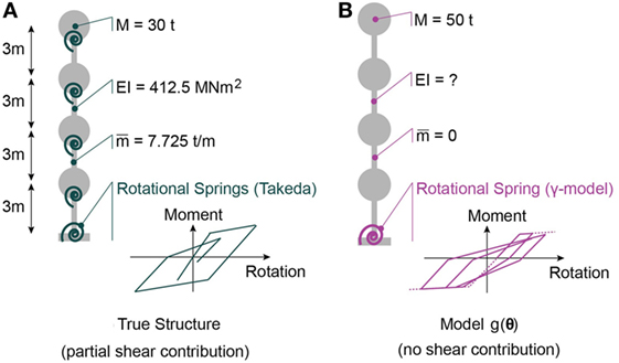
Figure 2. Description of lumped mass models representing the baseline (true) structure (A) as well as model g(.) for which parameters θ are identified (B). Identification is performed on states before and after main earthquake. Behavior during aftershock is predicted.

In reality, models are simplified and approximate representations of reality. Therefore, the model instance g(.) that is used to identify values of the parameter vector θ has a model bias with respect to the true structure. The mass is lumped at the floors and estimated to be 50 t per floor. The structure is assumed to be perfectly moment-resisting, meaning no rotation restraint of the lumped masses is considered. In addition, the plasticity is localized with a non-linear hysteretic spring at the base level. The hysteretic behavior is assumed to be defined by the Gamma-model (Lestuzzi and Badoux, 2003). A global damping coefficient of 5% is assumed for the structure. The structure that is identified using the three investigated methodologies is shown in Figure 2B.

Parameters θ that are identified for model g(.) are the stiffness EI as well as the parameters of the γ-model governing the behavior of the rotational spring: stiffness (k_rot), yield moment (M_y), post-yield stiffness (hard), and the gamma-factor (γ). Thus, in total five parameters are identified based on simulated measurements (see Table 1). The remaining parameters defining the model g(.) are assumed to be known and add to the model error. Initial ranges for the parameter values are given in Table 1. Prior distributions related to parameter knowledge are taken to be uniform, which corresponds to a realistic scenario.

TABLE 1

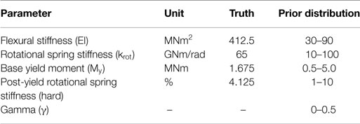
Table 1. True values and prior distributions of the parameters to identify.

Ground Motion Characteristics

The simulated earthquake-aftershock sequence, for which predictions will be performed, are shown in Figure 3. The selected main shock is the Alkion, Greece, earthquake from February 24th, 1981. The selected aftershock is the Izmit, Turkey, aftershock from September 13th, 1999. The two ground motions are simulated with a non-linear time-history analysis in a sequential way, with 1 s of zero-acceleration between the two signals. The true behavior of the base spring is shown in Figure 3 for the main shock and the aftershock.

FIGURE 3

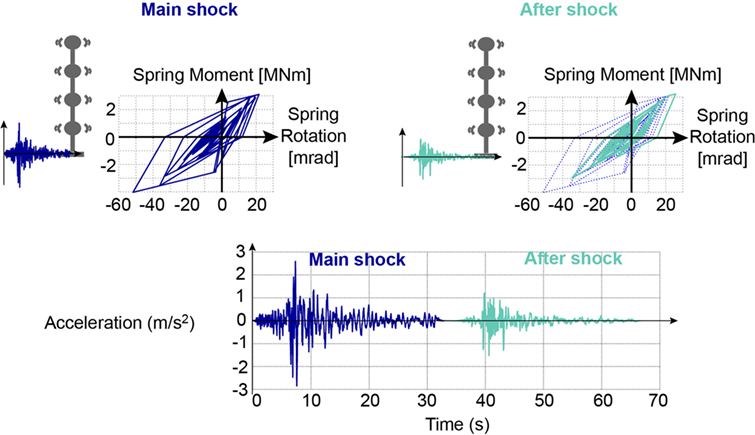
Figure 3. Simulation of Mainshock and Aftershock sequence using the true model for simulated measurements. For identification, mainshock and aftershock are run for each model instance.

The measurement uncertainty is simulated by randomly adding an instance of the chosen measurement uncertainty to each measured quantity. The measurement error related to natural frequencies follows a normal n(0,1.5%) distribution while measurement error on modal displacements is estimated to be defined by a n(0,5.0%) distribution.

Identification Scenarios

Three identification methodologies are compared in this paper (see BACKGROUND): (i) TBMU with zero-mean independent normal likelihood functions; (ii) MBMU with a non-zero-mean uniform (generalized normal distribution with an L∞-norm) biased likelihood function; and (iii) EDMF with thresholds that are derived from biased uncertainty distributions. In inverse tasks, such as structural identification, epistemic uncertainty resulting from the discrepancy between model predictions and true structural behavior has an important influence.

There are two approaches to determine the model uncertainty related to such discrepancies. Either engineering heuristics can help to estimate conservative bounds on the model uncertainty, or measurement data can be used to infer the uncertainty. In the second case, supplementary parameters θ_i need to be identified.

A total of eight structural identification applications are compared. The three structural identification methodologies are implemented for three scenarios based on how uncertainties are taken into account. A summary of the eight applications is provided in Table 2.

TABLE 2

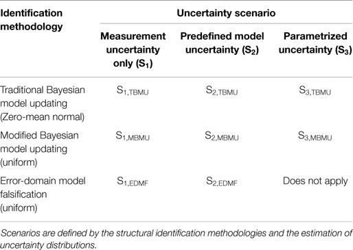
Table 2. Eight identification scenarios are used for comparisons.

Two uncertainty scenarios involve predefined uncertainty ranges. First, model error is ignored (Scenarios S₁ in Table 2) and a zero-mean normal measurement uncertainty is defined in accordance with the measurement errors that are added to the true model in order to obtain simulated measurements (see Ground Motion Characteristics). The second uncertainty scenario involves a distribution that combines measurement uncertainty and model uncertainty (Scenarios S₂ in Table 2). Model uncertainty is defined as a uniform distribution that is derived based on the true model error values. The true model error is defined by Eq. 10. Absolute uncertainty values that are used in the identification process are obtained by multiplying relative model errors by the model prediction with mean parameter values, $g\left(\overline{\mathrm{\theta }}\right)$. Therefore, the discrepancy between truth and model predictions with true parameter values, g(θ*), is divided by model predictions resulting from mean parameter values in Eq. 10.

${\mathrm{\epsilon }}_{\text{model}}=\frac{\text{Truth}-g\left({\mathrm{\theta }}^{\ast }\right)}{g\left(\overline{\mathrm{\theta }}\right)}$ (10)

The third uncertainty scenario involves parametrization of uncertainties. The initial ranges for relative uncertainty SD and mean are 0–100%. EDMF relies on engineering judgment to estimate combined uncertainty; therefore, uncertainty identification is limited to BMU methodologies.

Four separate model uncertainty distributions are derived for: initial frequencies, initial MAC values, post-earthquake frequencies, and post-earthquake MAC values. Model uncertainty distributions are obtained as a uniform distribution between the minimum and the maximum error calculated for the three first modes that are used for identification. Likelihood functions for TBMU and MBMU that are derived from combining predefined measurement and model uncertainties based on Eq. 10 for natural frequencies before and after the main shock are shown in Figure 4. Falsification thresholds that are used in EDMF are equivalent to the boundaries of the MBMU. The uncertainty distribution that is calculated using the true model is not zero-mean. Thus, a zero-mean normal distribution that is fitted using such a biased distribution results in a wider distribution when compared to the uniform likelihood function related to MBMU (see Figure 4).

FIGURE 4

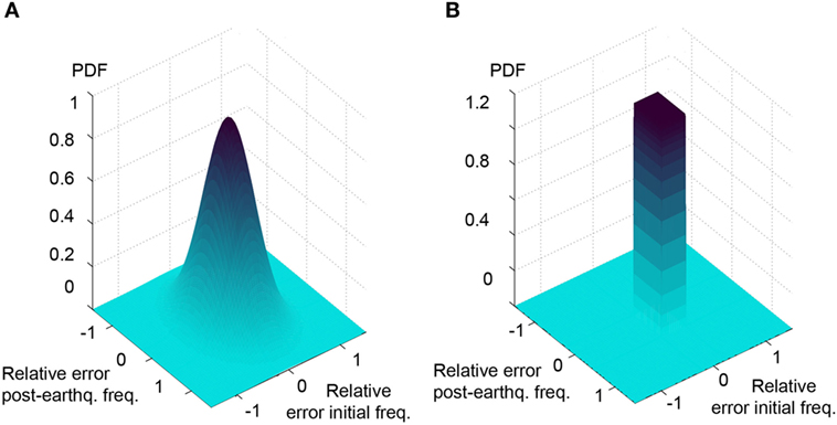
Figure 4. Likelihood functions for traditional Bayesian model updating (TBMU) (left) and modified Bayesian model updating (MBMU) (right) calculated using true model error values (Scenario S₂ in Table 2). (A) Zero-mean normal likelihood function for TBMU. (B) Non-zero-mean uniform likelihood function for MBMU.

Three vibration modes are used for identification. Therefore, in order to limit the number of uncertainty distributions, single distributions are calculated for initial natural frequencies, post-earthquake natural frequencies, initial mode-shapes, and post-earthquake mode-shapes. Therefore, when uncertainties are parametrized for BMU applications, additional parameters need to be identified. For TBMU, SD for four independent zero-mean normal distributions are identified (S_3,TBMU in Table 2). For MBMU, eight additional uncertainty parameters are identified, being the mean and SD of uniform likelihood functions (S_3,MBMU in Table 2). For numerical stability reasons, uniform likelihood functions are approximated with generalized Gaussian distributions with a norm (κ) of 250 (see Eq. 7).

Sampling of the Parameter Space

Markov-chain Monte-Carlo sampling is used for the applications of Bayesian model updating (TBMU and MBMU). A Metropolis–Hastings algorithm (Hastings, 1970) is used to guide the random walk through the multi-dimensional parameter space. The convergence of the random walk method to the posterior distribution depends on the parameters that are chose for the Metropolis–Hastings algorithm. For identification scenarios with predefined uncertainty, 30,000 accepted samples are used. If uncertainty is parametrized, the higher number of parameters is accounted for by using 60,000 samples.

Grid sampling is used for EDMF. An initial model population is generated by dividing the parameter space (see Table 1) with a regular grid. The initial range of flexural stiffness is divided into 18 intervals, rotational spring stiffness into 12 intervals, base yield moment and post-yield spring stiffness into eight intervals, and Gamma-value into 5 intervals. Thus, the initial model population is composed of 120,042 parameter combinations. Grid sampling results in independent simulations for each parameter combination (no guided search or stochastic sampling), which favors parallel computing schemes.

Identification Results

The first uncertainty scenario (see Table 2) involves ignoring model uncertainty, and defining the total uncertainty using zero-mean normal measurement uncertainty, N(0,1.5%). Although the total uncertainty is underestimated, TBMU provides identification results (S_1,TBMU). The 30,000 samples that are obtained using MCMC sampling and that define the posterior probability of parameter values are shown in Figure 5. The identification result is precise, as the scatter is low compared to the initial (or prior) parameter range. This is true for linear parameters (Figure 5A) as well as for non-linear parameters (Figure 5B). However, the identification result is biased from the true parameter values. If model uncertainty, which is usually systematic and biased, is ignored, inaccurate identification results are obtained.

FIGURE 5

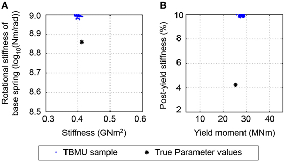
Figure 5. Posterior distribution of parameter values obtained using traditional Bayesian model updating (TBMU) ignoring model uncertainty (S_1,TBMU in Table 2). The TBMU parameter identification result is precise, yet biased and inaccurate. Modified Bayesian model updating and error-domain model falsification falsified the entire model class. (A) Linear parameters. (B) Non-linear parameters.

Modified Bayesian model updating fails to provide a starting point for MCMC sampling when model uncertainty is ignored (S_1,MBMU). For100,000 randomly selected starting points in the parameter space, no parameter combination provides results that return a likelihood other than 0. Therefore, it is concluded that using MBMU, the model class, g(.), is rejected. Model class rejection indicates either a wrong model, a wrong selection or estimation of model parameters, or an underestimation of uncertainties.

Using EDMF, the initial model population sampled from the parameter space using a regular grid is entirely falsified when model uncertainty is ignores (S_1,EDMF). In a similar way to MBMU, this result indicates a misevaluation of the uncertainty or a wrong model class. The capacity to falsify entire model classes increases the robustness of structural identification by reducing the risk of biased results.

The second uncertainty scenario involves predefined uncertainty with correctly estimated measurement and model uncertainty (S₂ in Table 2). The identification results for linear parameters that are obtained from the three studied identification techniques are shown in Figure 6. The tails of the zero-mean normal likelihood function of TBMU are widespread compared with the bounds of the uniform likelihood function for MBMU and EDMF (see Figure 4). Therefore, the identification results that are obtained using TBMU (Figure 6A) are less precise than EDMF and MBMU. MBMU provides accurate and precise identification of linear parameters (Figure 6B).

FIGURE 6

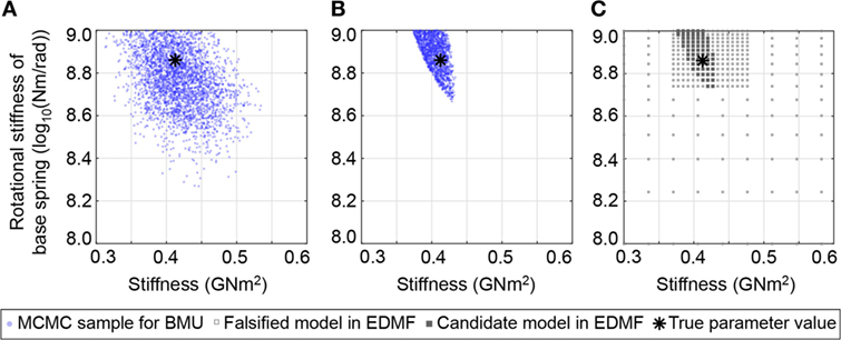
Figure 6. Identification results for linear parameters resulting from correctly estimated model uncertainty for S_2,TBMU (A), S_2,MBMU (B), and S_2,EDMF (C), as defined in Table 2. Modified Bayesian model updating (MBMU) and error-domain model falsification (EDMF) provide similarly accurate results.

Prediction of modal properties related to the initial state exclusively depend on linear parameters, which are model stiffness and rotational spring stiffness. Due to a small interval of identified values for structural stiffness compared to the initial range (8%), grid sampling for EDMF is re-evaluated using a sequential scheme: based on the results of the coarse grid (120,402 sample, see The Measurement Uncertainty Is Simulated by Randomly Adding an Instance of the Chosen Measurement Uncertainty to Each Measured Quantity. The Measurement Error Related to Natural Frequencies Follows a Normal N(0,1.5%) Distribution While Measurement Error on Modal Displacements Is Estimated to Be Defined by a N(0,5.0%) Distribution. Identification Scenarios), the linear parameters are resampled in the region containing candidate models, thereby increasing the total number of samples to 21,204 (Figure 6C). EDMF explicitly allows engineers to sequentially add information and model instances (Pasquier and Smith, 2016).

Identified parameter ranges for EDMF are contained within identified ranges for MBMU. Unlike MBMU, which involves a MCMC sampling scheme, EDMF relies on discrete grid sampling of the parameter space. Therefore, MBMU gives a more refined result of the identified parameter space contour.

While parameter identification is precise for linear parameters, identification of non-linear parameters fails to provide precise results (see Figure 7). The widespread tails of the zero-mean normal distribution undermine non-linear parameter identification for TBMU (see Figure 7A). However, even for uniform model uncertainty distributions (see Figure 4B), no significant reduction in the parametric uncertainty related to non-linear parameters can be obtained (see Figure 7B for MBMU and Figure 7C for EDMF). This is to be expected since all measurements are made in the linear range.

FIGURE 7

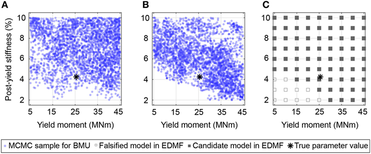
Figure 7. Identification results for non-linear parameters resulting from correctly estimated model uncertainty. Parametric uncertainty cannot be reduced significantly. (A) Traditional Bayesian model updating. (B) Modified Bayesian model updating. (C) Error-domain model falsification (EDMF).

The third uncertainty scenario involves parametrizing the likelihood function (S₃ in Table 2). The identified SD values exceed the values that are derived using the true model. SDs of the zero-mean normal likelihood function (S_3,TBMU) are shown in Figure 8 for initial and post-earthquake frequencies, f_ini and f_peq. The SD is provided as a relative value, as proposed in Eq. 10. Uncertainty parameter identification provides more precision, when compared to the prior distribution (uniform between 0 and 1). However, in general terms, uncertainty values are overestimated when they are parametrized.

FIGURE 8

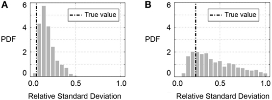
Figure 8. Identification results for parametrized uncertainties in traditional Bayesian model updating application (S_3,TBMU in Table 2). The SD of a zero-mean normal distribution is identified. (A) Likelihood function for initial frequency (f_ini) and (B) likelihood function for post-earthquake frequency (f_peq).

For TBMU, the SD of a zero-mean normal distribution is treated as an uncertain parameter. However, the limited number of measurements undermines identifiability of structural parameters in addition to likelihood function parameters. Thus, no reduction in the structural parameter uncertainty is obtained for either linear or non-linear parameters and the results for parameter identification are not reported.

Modified Bayesian model updating relies on uniform likelihood functions with a constant probability inside bounds and zero probability outside the bounds. As MBMU allows biased uncertainty distribution (not centered on 0), parametrizing uncertainty leads to eight additional parameters for scenario S_3,MBMU (see Table 2): lower and upper bounds on the likelihood function for natural frequencies and MAC values before and after the earthquake. The identification results for parametrized bounds to uniform likelihood functions in MBMU are reported in Figure 9 for initial and post-earthquake frequencies. The distribution of identification results indicates higher precision for the lower bound than for the upper bound. Also, values for lower bounds are accurately identified, while upper bounds tend to be overestimated. Overestimated uncertainty bounds result in conservative parameter identification. In general, the distribution of identified uncertainty bounds hinders a precise identification of parameter values.

FIGURE 9

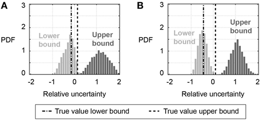
Figure 9. Identification of parametrized bounds to the L∞ norm likelihood function implemented in modified Bayesian model updating (S_3,MBMU in Table 2). (A) Bounds to uniform likelihood function for initial frequency (f_ini) and (B) bounds to uniform likelihood function for post-earthquake frequency (f_peq).

In this case, 12 measured quantities are available: natural frequencies and mode-shapes of the first three modes before and after the earthquake. Identifying SDs for TBMU adds four likelihood function parameters to the five structural parameters. Identifying bounds for uniform likelihood functions in addition to parameter values would require the identification of a total of 13 parameters. In addition, long computation times, which increase with the number of parameters (higher number of samples are needed to get stable results), a high number of parameters is unidentifiable when limited number of measurements is available. Therefore, in such scenarios, uncertainties need to be identified prior to the identification task.

When such error estimations take the form of bounds on uniform distributions, the identification results may lead to the conclusion that the model class is wrong or the error underestimated. Underestimating the uncertainty can lead to biased identification results when error estimations are taken to be Gaussian, as it is the case using TBMU when model error is ignored. Such biased identification potentially leads to wrong predictions, as shown in the next section.

Prediction

Identification of parameter values is an intermediate step when the goal is to predict behavior. In this section, identification methodologies are compared with respect to the accuracy and precision of behavior predictions. Predictions are carried out for base moment and top displacement during an aftershock. Since loading conditions differ from measurement conditions (modal properties), extrapolation is needed.

When extrapolation is carried out, the model error potentially differs from the model error that is used for identification. For instance, top displacement depends linearly on stiffness, while model properties depend on the square-root of stiffness. Therefore, model error should be redefined for extrapolation-based prognosis.

Model prediction uncertainty is estimated from true model predictions using Eq. 10 in a similar way than model uncertainty is estimated for identification. Calculating model error using Eq. 10 returns a single value for prediction error (−55% for predicted maximum base moment and −73.5% for predicted maximum top displacement). Therefore, model uncertainty is assumed to be uniformly distributed between the estimated prediction errors and 0. Model uncertainty, U_g in Eq. 4, is thus estimated to be part of the interval [−55%, 0%] for base moment and [−73.5%, 0] for top displacement. Estimated prediction uncertainties are larger than model uncertainty related to modal properties, which is estimated for identification. Hence, the need for re-evaluating model uncertainties to achieve robust predictions is underlined.

For identification scenarios that ignore model error (S₁ in Table 2), the prediction range is taken without adding model uncertainty. For identification scenarios that involve parametrizing the uncertainty distributions, model prediction uncertainties need to be re-estimated as well, as identified errors are limited to the measurement conditions. The modeling error is applied to identification scenarios (b) and (c), Figure 10. A Monte-Carlo scheme with 5 million samples is used to combine parametric prediction uncertainty with model prediction uncertainty.

FIGURE 10

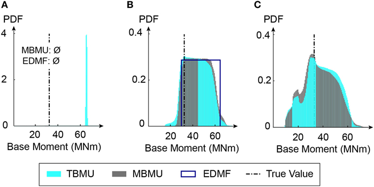
Figure 10. Comparison of predicted absolute maximum base moment during an aftershock for tested identification scenarios. If model errors are ignored (S₁ in Table 2), error-domain model falsification (EDMF) and modified Bayesian model updating (MBMU) indicate that the wrong model class is used (A). The vertical axis (probability density function) for measurement uncertainty (A) is increased for better readability. (B) Predefined uncertainty. (C) Parameterized uncertainty.

Predictions related to maximum absolute base moment values are presented in Figure 10. If model error is ignored (see Figure 10A), MBMU and EDMF indicate a wrong model class. Posterior parameter distributions for TBMU without model errors result in biased predictions compared to the true aftershock base moment.

Error-domain model falsification assumes uniform prediction intervals based on bounds that are derived using a target prediction probability of 0.95. For predictions based on BMU, the complete prediction distribution is reported. The prediction results based on the true model error are accurate, as the true values are included in the prediction distributions. Prior parameter distributions without identification result in a prediction interval of 6–68 kNm for base moment. Thus, prediction range resulting from EDMF is reduced to 55% of the initial prediction range. For parametrized uncertainties (Figure 10C), no reduction in the prediction range can be obtained, given the non-identifiability of model parameters.

Figure 11 shows the prediction results related to the top displacement during an aftershock. Again, the prediction ranges yield similar results. TBMU without model error (S_1,TBMU in Table 2), Figure 11A, provides precise yet inaccurate biased results. The prediction range obtained from EDMF (S_2,EDMF in Table 2) is 14% of the initial prediction range and provides accurate thus, robust, results. Also, the prediction ranges resulting from parametrized uncertainties are high (see Figure 11). For top displacement predictions, the maximum likelihood estimates provided by BMU scenarios are acceptable. However, given the results for base moments, it appears best to sacrifice prediction precision in order to increase prediction accuracy, through use of EDMF, Figure 11.

FIGURE 11

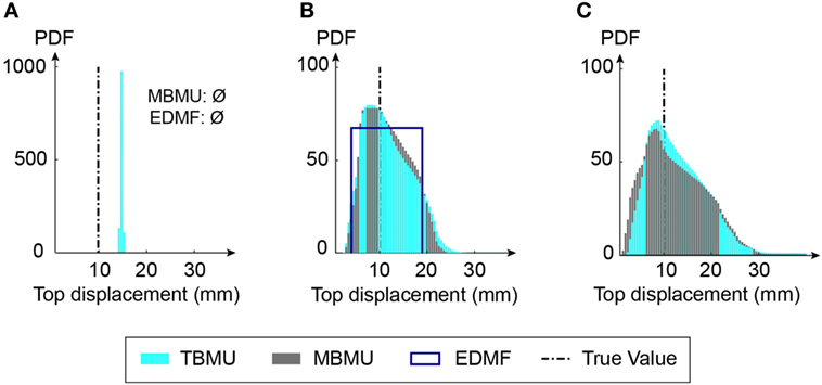
Figure 11. Comparison of predicted absolute maximum top displacements during an aftershock for tested identification scenarios. If model errors are ignored (S₁ in Table 2), error-domain model falsification (EDMF) and modified Bayesian model updating (MBMU) indicate that the wrong model class is used (A). The vertical axis (probability density function) for measurement uncertainty (A) is increased for better readability. (B) Predefined uncertainty. (C) Parameterized uncertainty.

Estimating model errors correctly is challenging in full-scale applications. Therefore, the robustness of EDMF results with regard to misevaluated model uncertainty is assessed. As EDMF results are based on grid sampling, changing model uncertainty values does not require new model simulations. EDMF thereby enables the engineer to adapt and change model uncertainties when increased knowledge of the structure is acquired, for instance, through in situ inspections.

The influence of model uncertainty levels is first assessed with respect to the number of candidate models that are found. As can be seen in Figure 12, no candidate models are found for model errors that are lower than 95% of the model uncertainty that is estimated using the true values in Eq. 10. This source of robustness is very useful in applications on full-scale structures. If model errors are overestimated, higher numbers of incorrect models are accepted.

FIGURE 12

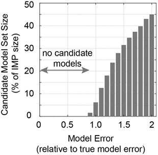
Figure 12. Size of the candidate model set evaluated for changing levels of model error estimations.

Even more important than identification, the prediction robustness of EDMF with regard to misevaluation of model errors is assessed in Figure 13. If model uncertainty is underestimated, by more than 10%, no candidate models are found. This feature of EDMF (and MBMU) leads to robust predictions. TBMU lacks this source of robustness, as identification results are found even for 0% model error (see Figure 6). Thus, uniform PDFs for combined model and measurement uncertainties are appropriate and robust for situations with unknown and varying uncertainty correlation values. Predictions that involve extrapolation are robust with respect to large, biased, and correlated uncertainties. However, overestimation of model error reduces the precision of prediction ranges. Therefore, EDMF and MBMU sacrifice precision for increased accuracy (or robustness).

FIGURE 13

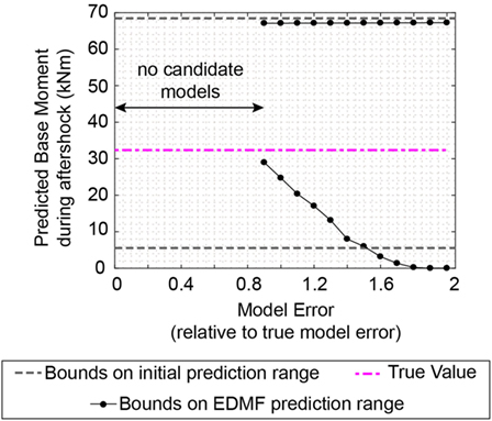
Figure 13. Evolution of the maximum base moment prediction range during an aftershock. No candidate models were found for model uncertainties smaller than 90% of the model uncertainty derived using the true model.

Summary and Discussion

Three structural identification methodologies are compared in terms of parameter identification and behavior prediction. Through varying scenarios for taking model uncertainty into account (no model uncertainty, predefined model uncertainty and parametrized model uncertainty), the data-interpretation methodologies are tested with respect to accuracy of prediction intervals that involve extrapolation from linear modal properties (used for identification) to non-linear time-history predictions. Traditional assumptions, such as zero-mean normal uncertainties are found to be inappropriate in such applications.

Simulated measurements from a simplified structure are used to test three structural identification methodologies. Upper bounds of the usefulness of structural identification using non-linear behavior models from linear measurements are obtained. Model uncertainties, such as ignoring shear contribution, changing hysteretic rules and ignoring springs on upper stories (as shown in Figure 2) are quantified. Non-linear time-history analyses are path dependent. Thus, a significant amount of uncertainty is related to the loading history of non-linear springs. Modal measurements do not provide information about past maximum encountered strains or displacements. However, unlike base shear or top displacements, modal properties can be measured quickly and at low cost. Therefore, this paper gives an upper bound estimation for the efficiency of identifying linear parameters for non-linear analyses.

Traditional assumptions for structural identification are shown to be inappropriate. However, future work on full-scale structures and models with increased complexity is needed to validate the accuracy of structural identification methodologies that are based on uninformed (uniform) uncertainty distributions.

Conclusion

Structural identification with non-linear models based on linear measurements is a challenging task. Three identification techniques that provide populations of solutions are reviewed and compared. The following conclusions are drawn:

– Uniform probability distributions for combined model and measurement uncertainties are appropriate for situations with unknown and varying uncertainty correlation values. Predictions that involve extrapolation are robust with respect to large, biased and correlated uncertainties. Prediction precision is sacrificed to maintain accuracy.

– Traditional Bayesian model updating that relies on non-uniform uncertainty predictions can result in biased prediction ranges. Maximum likelihood estimates should, therefore, be avoided. In addition, unlike MBMU and EDMF, TBMU fails to reject wrong model classes, which can result in wrong identification as well as incorrect predictions.

– Adding prediction error is essential for predictions of structural behavior. For prognosis of building responses to actions that differ largely from measurement conditions, prediction uncertainty can be larger than identification uncertainty.

– Parametrized uncertainties in MBMU (L∞ norm) provide conservative estimates of upper bounds of the correct model uncertainties. However, small numbers of measurements can undermine identification of parameter values along with parametrized uncertainty distributions.

– For parameters that are related to non-linear behavior, the precision of structural identification based on linear measurements (natural frequencies) is understandably lower than for linear parameters. Nevertheless, prediction ranges can be reduced by 30% (for base moments) to 90% (for top displacements) using EDMF.

Author Contributions

YR elaborated the application of the methodology to the context of non-linear predictions with linear modal measurement data. PL assisted to the elaboration of the case study and wrote the code for non-linear dynamic simulation. Also, YR wrote the majority of the paper and conducted the research and simulations of the case study. IS was actively involved in developing and adapting the data-interpretation methodology and wrote parts of the contribution. All authors reviewed and accepted the final version.

Conflict of Interest Statement

The authors declare that the research was conducted in the absence of any commercial or financial relationships that could be construed as a potential conflict of interest.

Acknowledgments

This work was funded by the Swiss National Science Foundation under Contract No. 200020-169026. The authors thank Dr. Romain Pasquier and Sai Pai for their input and the reviewers for their constructive remarks.

References

Allemang, R. J., and Brown, D. L. (1982). “A correlation coefficient for modal vector analysis,” in Proceedings of the 1st International Modal Analysis Conference (Orlando: SEM), 110–116.

Google Scholar

Asgarieh, E., Moaveni, B., Barbosa, A. R., and Chatzi, E. (2017). Nonlinear model calibration of a shear wall building using time and frequency data features. Mech. Syst. Signal Process. 85, 236–251. doi: 10.1016/j.ymssp.2016.07.045

CrossRef Full Text | Google Scholar

Beck, J. L., and Au, S.-K. (2002). Bayesian updating of structural models and reliability using Markov chain Monte Carlo simulation. J. Eng. Mech. 128, 380–391. doi:10.1061/(ASCE)0733-9399(2002)128:4(380)

CrossRef Full Text | Google Scholar

Beck, J. L., and Katafygiotis, L. S. (1998). Updating models and their uncertainties. I: Bayesian statistical framework. J. Eng. Mech. 124, 455–461. doi:10.1061/(ASCE)0733-9399(1998)124:4(455)

CrossRef Full Text | Google Scholar

Behmanesh, I., Moaveni, B., Lombaert, G., and Papadimitriou, C. (2015). Hierarchical Bayesian model updating for structural identification. Mech. Syst. Signal Process. 64–65, 360–376. doi:10.1016/j.ymssp.2015.03.026

CrossRef Full Text | Google Scholar

Behmanesh, I., Moaveni, B., and Papadimitriou, C. (2017). Probabilistic damage identification of a designed 9-story building using modal data in the presence of modeling errors. Eng. Struct. 131, 542–552. doi:10.1016/j.engstruct.2016.10.033

CrossRef Full Text | Google Scholar

Beven, K., and Binley, A. (1992). The future of distributed models: model calibration and uncertainty prediction. Hydrol. Process. 6, 279–298. doi:10.1002/hyp.3360060305

CrossRef Full Text | Google Scholar

Brynjarsdóttir, J., and O’Hagan, A. (2014). Learning about physical parameters: the importance of model discrepancy. Inverse Probl. 30, 114007. doi:10.1088/0266-5611/30/11/114007

CrossRef Full Text | Google Scholar

Chellini, G., De Roeck, G., Nardini, L., and Salvatore, W. (2010). Damage analysis of a steel–concrete composite frame by finite element model updating. J. Construct. Steel Res. 66, 398–411. doi:10.1016/j.jcsr.2009.10.004

CrossRef Full Text | Google Scholar

Cheung, S. H., and Beck, J. L. (2009). Bayesian model updating using hybrid Monte Carlo simulation with application to structural dynamic models with many uncertain parameters. J. Eng. Mech. 135, 243–255. doi:10.1061/(ASCE)0733-9399(2009)135:4(243)

CrossRef Full Text | Google Scholar

Clinton, J. F., Bradford, S. C., Heaton, T. H., and Favela, J. (2006). The observed wander of the natural frequencies in a structure. Bull. Seismol. Soc. Am. 96, 237–257. doi:10.1785/0120050052

CrossRef Full Text | Google Scholar

Ebrahimian, H., Astroza, R., Conte, J. P., and de Callafon, R. A. (2017). Nonlinear finite element model updating for damage identification of civil structures using batch Bayesian estimation. Mech. Syst. Signal Process. 84(Part B), 194–222. doi:10.1016/j.ymssp.2016.02.002

CrossRef Full Text | Google Scholar

Fernández-Martínez, J. L., Fernández-Muñiz, Z., Pallero, J. L. G., and Pedruelo-González, L. M. (2013). From Bayes to Tarantola: new insights to understand uncertainty in inverse problems. J. Appl. Geophys. 98, 62–72. doi:10.1016/j.jappgeo.2013.07.005

CrossRef Full Text | Google Scholar

Galloway, B., Hare, J., Brunsdon, D., Wood, P., Lizundia, B., and Stannard, M. (2014). Lessons from the post-earthquake evaluation of damaged buildings in Christchurch. Earthq. Spectra 30, 451–474. doi:10.1193/022813EQS057M

CrossRef Full Text | Google Scholar

Goulet, J.-A., Kripakaran, P., and Smith, I. F. C. (2010). Multimodel structural performance monitoring. J. Struct. Eng. 136, 1309–1318. doi:10.1061/(ASCE)ST.1943-541X.0000232

CrossRef Full Text | Google Scholar

Goulet, J.-A., Michel, C., and Smith, I. F. C. (2013). Hybrid probabilities and error-domain structural identification using ambient vibration monitoring. Mech. Syst. Signal Process. 37, 199–212. doi:10.1016/j.ymssp.2012.05.017

CrossRef Full Text | Google Scholar

Goulet, J.-A., and Smith, I. F. C. (2013). Structural identification with systematic errors and unknown uncertainty dependencies. Comput. Struct. 128, 251–258. doi:10.1016/j.compstruc.2013.07.009

CrossRef Full Text | Google Scholar

Green, P. L., and Worden, K. (2015). Bayesian and Markov chain Monte Carlo methods for identifying nonlinear systems in the presence of uncertainty. Phil. Trans. R. Soc. A 373, 20140405. doi:10.1098/rsta.2014.0405

PubMed Abstract | CrossRef Full Text | Google Scholar

Hastings, W. K. (1970). Monte Carlo sampling methods using Markov chains and their applications. Biometrika 57, 97–109. doi:10.1093/biomet/57.1.97

CrossRef Full Text | Google Scholar

Jalayer, F., Asprone, D., Prota, A., and Manfredi, G. (2011). A decision support system for post-earthquake reliability assessment of structures subjected to aftershocks: an application to L’Aquila earthquake, 2009. Bull. Earthq. Eng. 9, 997–1014. doi:10.1007/s10518-010-9230-6

CrossRef Full Text | Google Scholar

Jeon, J.-S., DesRoches, R., Lowes, L. N., and Brilakis, I. (2015). Framework of aftershock fragility assessment–case studies: older California reinforced concrete building frames. Earthq. Eng. Struct. Dyn. 44, 2617–2636. doi:10.1002/eqe.2599

CrossRef Full Text | Google Scholar

Katafygiotis, L. S., and Yuen, K.-V. (2001). Bayesian spectral density approach for modal updating using ambient data. Earthq. Eng. Struct. Dyn. 30, 1103–1123. doi:10.1002/eqe.53

CrossRef Full Text | Google Scholar

Lam, H.-F., Hu, J., and Yang, J.-H. (2017). Bayesian operational modal analysis and Markov chain Monte Carlo-based model updating of a factory building. Eng. Struct. 132, 314–336. doi:10.1016/j.engstruct.2016.11.048

CrossRef Full Text | Google Scholar

Lestuzzi, P., and Badoux, M. (2003). “The gamma-model: a simple hysteretic model for reinforced concrete walls,” in Proceedings of the Fib-Symposium: Concrete Structures in Seismic Regions. Athens.

Google Scholar

Marshall, J. D., Jaiswal, K., Gould, N., Turner, F., Lizundia, B., and Barnes, J. C. (2013). Post-earthquake building safety inspection: lessons from the Canterbury, New Zealand, earthquakes. Earthq. Spectra 29, 1091–1107. doi:10.1193/1.4000151

CrossRef Full Text | Google Scholar

Marsili, F., Croce, P., Friedman, N., Formichi, P., and Landi, F. (2017). Seismic reliability assessment of a concrete water tank based on the Bayesian updating of the finite element model. ASME J. Risk Uncertain. Eng. Syst. B Mech. Eng. 3, 021004. doi:10.1115/1.4035737

CrossRef Full Text | Google Scholar

Michel, C., Zapico, B., Lestuzzi, P., Molina, F. J., and Weber, F. (2011). Quantification of fundamental frequency drop for unreinforced masonry buildings from dynamic tests. Earthq. Eng. Struct. Dyn. 40, 1283–1296. doi:10.1002/eqe.1088

CrossRef Full Text | Google Scholar

Moaveni, B., He, X., Conte, J. P., and Restrepo, J. I. (2010). Damage identification study of a seven-story full-scale building slice tested on the UCSD-NEES shake table. 32, 347–356. doi:10.1016/j.strusafe.2010.03.006

CrossRef Full Text | Google Scholar

Mucciarelli, M., Masi, A., Gallipoli, M. R., Harabaglia, P., Vona, M., Ponzo, F., et al. (2004). Analysis of RC building dynamic response and soil-building resonance based on data recorded during a damaging earthquake (Molise, Italy, 2002). Bull. Seismol. Soc. Am. 94, 1943–1953. doi:10.1785/012003186

CrossRef Full Text | Google Scholar

Muto, M., and Beck, J. L. (2008). Bayesian updating and model class selection for hysteretic structural models using stochastic simulation. J. Vibr. Control 14, 7–34. doi:10.1177/1077546307079400

CrossRef Full Text | Google Scholar

Nazari, N., van de Lindt, J. W., and Li, Y. (2015). Quantifying changes in structural design needed to account for aftershock hazard. J. Struct. Eng. 141, 04015035/1-10.

Google Scholar

Pai, S. G. S., and Smith, I. F. (2017). “Comparing three methodologies for system identification and prediction,” in 14th International Probabilistic Workshop (Gent: Springer), 81–95.

Google Scholar

Papadimitriou, C., Beck, J. L., and Katafygiotis, L. S. (1997). Asymptotic expansions for reliability and moments of uncertain systems. J. Eng. Mech. 123, 1219–1229. doi:10.1061/(ASCE)0733-9399(1997)123:12(1219)

CrossRef Full Text | Google Scholar

Pasquier, R., Goulet, J., Acevedo, C., and Smith, I. F. C. (2014). Improving fatigue evaluations of structures using in-service behavior measurement data. J. Bridge Eng. 19, 04014045. doi:10.1061/(ASCE)BE.1943-5592.0000619

CrossRef Full Text | Google Scholar

Pasquier, R., and Smith, I. F. C. (2015a). Robust system identification and model predictions in the presence of systematic uncertainty. Adv. Eng. Inform. 29, 1096–1109. doi:10.1016/j.aei.2015.07.007

CrossRef Full Text | Google Scholar

Pasquier, R., and Smith, I. F. C. (2015b). “Sources and forms of modelling uncertainties for structural identification,” in 7th International Conference on Structural Health Monitoring of Intelligent Infrastructure (SHMII). Torino.

Google Scholar

Pasquier, R., and Smith, I. F. C. (2016). Iterative structural identification framework for evaluation of existing structures. Eng. Struct. 106, 179–194. doi:10.1016/j.engstruct.2015.09.039

CrossRef Full Text | Google Scholar

Pastor, M., Binda, M., and Harčarik, T. (2012). Modal assurance criterion. Proc. Eng. 48, 543–548. doi:10.1016/j.proeng.2012.09.551

CrossRef Full Text | Google Scholar

Popper, K. R. (1959). The Logic of Scientific Discovery. London: Hutchinson.

Google Scholar

Priestley, M. J. N. (2000). “Performance based seismic design,” in Bulletin of the New Zealand Society for Earthquake Engineering 33.3, 325–346.

Google Scholar

Raghunandan, M., Liel, A. B., and Luco, N. (2015). Aftershock collapse vulnerability assessment of reinforced concrete frame structures. Earthq. Eng. Struct. Dyn. 44, 419–439. doi:10.1002/eqe.2478

CrossRef Full Text | Google Scholar

Raphael, B., and Smith, I. (1998). “Finding the right model for bridge diagnosis,” in Artificial Intelligence in Structural Engineering (Berlin: Springer), 308–319.

Google Scholar

Reuland, Y., Garofano, A., Lestuzzi, P., and Smith, I. F. (2015). “Evaluating seismic retrofitting efficiency through ambient vibration tests and analytical models,” in IABSE Conference–Structural Engineering: Providing Solutions to Global Challenges. Geneva.

Google Scholar

Réveillère, A., Gehl, P., Seyedi, D., and Modaressi, H. (2012). “Development of seismic fragility curves for mainshock-damaged reinforced-concrete structures,” in Presented at the 15th World Conference on Earthquake Engineering, Lisbon, 999.

Google Scholar

Robert-Nicoud, Y., Raphael, B., and Smith, I. F. C. (2005). System identification through model composition and stochastic search. J. Comput. Civil Eng. 19, 239–247. doi:10.1061/(ASCE)0887-3801(2005)19:3(239)

CrossRef Full Text | Google Scholar

Šidák, Z. (1967). Rectangular confidence regions for the means of multivariate normal distributions. J. Am. Stat. Assoc. 62, 626–633. doi:10.2307/2283989

CrossRef Full Text | Google Scholar

Simoen, E., Papadimitriou, C., and Lombaert, G. (2013). On prediction error correlation in Bayesian model updating. J. Sound Vibr. 332, 4136–4152. doi:10.1016/j.jsv.2013.03.019

CrossRef Full Text | Google Scholar

Smith, I. F. (2016). Studies of sensor-data interpretation for asset management of the built environment. Front. Built Environ. 2:8. doi:10.3389/fbuil.2016.00008

CrossRef Full Text | Google Scholar

Stedinger, J. R., Vogel, R. M., Lee, S. U., and Batchelder, R. (2008). Appraisal of the generalized likelihood uncertainty estimation (GLUE) method. Water Resour. Res. 44, W00B06. doi:10.1029/2008WR006822

CrossRef Full Text | Google Scholar

Takeda, T., Sozen, M. A., and Nielsen, N. N. (1970). Reinforced concrete response to simulated earthquakes. J. Struct. Div. 96, 2557–2573.

Google Scholar

Tarantola, A. (2006). Popper, Bayes and the inverse problem. Nat. Phys. 2, 492–494. doi:10.1038/nphys375

CrossRef Full Text | Google Scholar

Vanik, M. W., Beck, J., and Au, S. (2000). Bayesian probabilistic approach to structural health monitoring. J. Eng. Mech. 126, 738–745. doi:10.1061/(ASCE)0733-9399(2000)126:7(738)

CrossRef Full Text | Google Scholar

Worden, K., and Hensman, J. (2012). Parameter estimation and model selection for a class of hysteretic systems using Bayesian inference. Mech. Syst. Signal Process. 32, 153–169. doi:10.1016/j.ymssp.2012.03.019

CrossRef Full Text | Google Scholar