Prioritization Scheme for Proposed Road Weather Information System Sites: Montana Case Study

Introduction

Weather presents considerable challenges to highway agencies both in terms of safety and operations. From a safety standpoint, snow, ice, and other forms of precipitation may reduce pavement friction, increasing the potential for crashes when vehicles are traveling too fast for the conditions. From an operations standpoint, heavy snow storms may affect the connectivity of the highway network due to closures that need to be cleared in an efficient and timely fashion. Further, travelers should be informed about unusual pavement conditions and road closures on time to minimize the effect of adverse weather on the safety and mobility of the traveling public. For the aforementioned reasons, road weather information has become increasingly important for highway agencies particularly in regions that experience harsh winter weather conditions. Road Weather Information System (RWIS) consists of the hardware, software, and communications interfaces to collect and transfer road weather observations from or near the roadway to a display device at the user’s location (John et al., 2005). Today, most environmental sensor stations (ESS) for RWIS include various atmospheric sensors, some form of pavement sensor, and camera imaging. Additional sensors are also being added to some ESS locations to measure traffic volumes, traffic speeds, and vehicle classifications and weights (Hawkins and Albrecht, 2014).

Road weather information has been used by highway agencies in many applications such as winter maintenance, traveler information, and other weather-related intelligent transportation systems (ITS) applications. Data adequacy, reliability, and geographic coverage are critical attributes to consider for these transportation applications. Highway agencies are often faced with the challenge of selecting a limited number of ESS sites from a larger pool of proposed sites given the limited budgets available. This process has been largely subjective in practice, relying on the expertise and judgment of the agency staff involved. Therefore, there is a need for an objective prioritization scheme for proposed ESS stations, which should guide future RWIS expansion and ensure maximum utility (benefits) from new ESS installations.

Background

Environmental sensor station siting for RWIS has typically been a mostly subjective practice relying on local expert input, but a few attempts to make the process more objective have been documented.

General Guidance

The most recent Federal Highway Administration (FHWA) ESS Siting Guidelines (Manfredi et al., 2008) provide details concerning local siting, but little specific guidance for macro-scale geographic ESS placement beyond relying on DOT personnel and meteorologists. In general, the authors state that the placement of regional ESS should be on relatively flat, open terrain on the upwind side of the road.

Zwahlen et al. (2003) have identified many additional factors to consider when determining the placement of ESS including: climactic history, road class, traffic volumes, locations with high grades, crash history, and common storm pattern movement directions. While these factors are listed, a method for using them for geographic placement is not described in the report.

Researchers in North Dakota (Surface Transportation Weather Research Center, 2009) determined that a 30-mile radius coverage area should not be exceeded in order to discern finer scale weather patterns given North Dakota’s land-use and terrain. This is in-line with the FHWA guidelines recommendation of up to 20–30 miles for regional ESS (Manfredi et al., 2008). Using this general guideline and the existing ESS network, the researchers provided 18 additional recommended ESS locations to ensure more comprehensive coverage.

Systematic Approaches

Efforts in recent years have attempted to develop siting procedures that involve somewhat more objective and analytical means to determine geographic ESS placement. Analyzing the potential placement of 10 ESS in the Austin, Texas region, Jin et al. (2014) developed a placement optimization model that was driven primarily by weather-related crash history. The authors developed a safety concern index based on past weather-related crash occurrence then spatially optimized the placement of the 10 ESS to obtain the greatest risk coverage assuming a 10 mile area coverage radius per ESS.

During the initial design of Alberta’s RWIS network (Pinet and Lo, 2003) and a later expansion (Pinet and Bielkiewicz, 2009), the authors described the geographic siting procedures considering many factors. Topography, hydrology, meteorological zones, winter crash statistics, traffic volumes, and expertise from local meteorologist helped define influence areas for each ESS as well as the overall placement of the RWIS network. The initial RWIS locations were limited to the National Highway System and the expansion designs branched out from the initial placements.

Kwon and Fu (2013) developed geographic ESS placement methods based on multiple factors including surface temperature variability, mean surface temperatures, precipitation amounts, traffic volumes, crash rates, and highway classification. The authors also investigated case studies of their methods using different combinations of the placement factors for Ontario, Canada. The study area was first broken into equal sized cells for analysis, next only cells containing the relevant road network were considered as candidates for ESS placement, and then the analyses using the factors above were performed resulting in the candidate locations. The placement model outputs were then shown with the highest 140 ranked candidate locations highlighted and grid shading according to the prioritization from a combination of all factors.

Yang and Regan (2014) developed a methodology to prioritize the placement of ESS for RWIS in South Korea. Their methods for prioritizing placement of ESS includes factors related to snow vulnerability analysis, winter crash statistics, traffic volumes, and the presence of nearby cameras. The initial areas prone to snow were identified by personnel in regional offices and additional snow vulnerability analysis was performed on these areas. Next, these areas were reduced to eliminate places that already had ESS or nearby automatic weather stations that were placed appropriately to provide ESS type road weather information. Finally, the remaining areas were prioritized by considering winter crash history, traffic volumes, and whether or not a camera was installed nearby.

This research effort aims to build upon and expand the knowledge base that has begun to be constructed by these studies while focusing on the unique modeling approach proposed within for Montana.

Objective

The research presented in this paper aims at developing a model for assessing the merit of proposed new ESS sites which could serve as a guide for RWIS system expansion in a region or at the state level. Such a model can help transportation agencies in prioritizing the installation of new ESS sites on a regular basis. The model could also be used in finalizing the exact location of a proposed site along a specific corridor to ensure an optimum output is obtained.

Proposed Prioritization Scheme

In any given year, multiple sites may be proposed for installation of new ESS stations as part of an RWIS system expansion. Given that there are limited resources available, an agency is usually required to select only a few sites out of the proposed list of sites where weather data is deemed most needed. This process is mostly subjective in nature, and agency personnel are often faced with the challenge of coming up with a semi-objective rankings for the proposed sites which may help them in making this decision. Objective rankings would require the consideration of many factors that are all important in determining the merit of ESS installation at a particular site.

In this research, the proposed scheme for assessing the merit of a proposed ESS site takes into account the following considerations.

1. Weather conditions;

2. highway network served;

3. expected safety benefits;

4. geographic coverage of ESS stations in surrounding areas;

5. other opportunistic factors (OF).

Each of the above considerations is discussed briefly in the following sections.

Weather Conditions

Weather is one of the most important determinants of merit for new ESS sites. Both severity and variability in meteorological conditions are important considerations in this determination. From the severity perspective, weather data are more valuable and satisfy a larger need in areas where extreme winter weather conditions exist. For example, information on the form (snow, ice, rain, etc.) and amount of precipitation is critical for winter maintenance operations and ITS safety applications. On the other hand, variability of weather conditions in the area surrounding a proposed site is also important in assessing the need for a new adjacent ESS site. Specifically, if weather conditions do not vary significantly in the area surrounding a proposed site, then information from surrounding existing ESS stations may reasonably be used in predicting weather conditions at the new site. However, this may prove to be impractical should significant variability in weather conditions exist in the area surrounding the proposed site, such as when topography and terrain notably change over a relatively short distance.

Highway Network Served

Road Weather Information System programs are primarily intended to provide weather data for the highway system and its associated applications. As such, the role of an ESS station in remote areas where no major highways exist may not be as significant as that of a station that is located in developed areas with extensive highway network surrounding the ESS site.

Expected Safety Benefits

Adverse weather conditions can negatively affect safety on highways and result in higher frequencies of weather-related crashes. The availability of real-time weather data is critical for highway agencies to ensure safer roads by providing timely winter maintenance and/or alerting drivers to hazardous situations via traveler information systems and ITS warning devices. Therefore, higher instances of weather-related crashes along highway segments surrounding a proposed site may reflect a need for timely weather data.

Geographic Coverage of ESS Stations

Another consideration in assessing the need for a new EES station at a proposed site is the geographic coverage of existing ESS stations in the area. In areas where ESS stations are sparse and farther apart, the need for new installations becomes more evident as weather data there may be especially valuable in the absence of other ESS. Likewise, if the area is well served by ESS stations, justifying a new installation may be difficult.

Other OF

Power and communications are essential for the operation of ESS stations. Therefore, the availability and ease of access to power and communications often have implications on installation costs and feasibility and should be considered in assessing the merit of a proposed ESS site.

Structure of Proposed Model

In this section, the formulation of the proposed model is discussed along with the procedures developed for quantifying different model variables. The overall merit (OM) is a rank on a scale of 0–1.0 which will serve as an indicator of the merit (or the need) associated with a proposed new site. The OM can be calculated using the following equation:

$\text{OM}=w_1(\text{WI})+w_2(\text{CI})+w_3(\text{TI})+w_4(\text{GC})+w_5(\text{OF})$

where WI is the weather index, CI is the crash index, TI is the traffic index, GC is the geographic coverage index, OF is the opportunistic (situational) factors, and w₁, w₂, w₃, w₄, and w₅ are the weights associated with model variables that should be selected to reflect the agency preferences and priorities.

The weights assigned to the different terms in the OM model are determined using input from agency staff who are concerned with RWIS applications and maintenance. The use of collective staff judgment in assigning these weights will ensure that agency priorities are reflected in the OM model.

Weather Index

The WI accounts for all meteorological variables that are deemed important in a new ESS installation. As discussed earlier, those variables are indicators of the severity and variability in weather conditions at the proposed site. The WI is calculated using the following equation:

$\mathrm{WI}=a_1(\text{FT})+a_2(\text{RF})+a_3(\text{SI})+a_4(\text{TG})+a_5(\text{SG})$

where FT is the freezing temperature, measured as the proportion of time during the year with minimum temperature below 32° Fahrenheit, RF is the annual rainfall accumulation score, SI is the monthly snowfall intensity score, TG is the temperature relative gradient score, SG is the snowfall relative gradient score, and a₁, a₂, a₃, a₄, and a₅ are the weights associated with model variables which should be selected to reflect the agency preferences and priorities.

The first variable in the above equation, FT, is calculated as the number of months during the year with average minimum temperature less than 32° divided by 12 (months in a full year). The second variable, RF, is a score which represents the expected total annual accumulation of rainfall at the proposed ESS site. In regard to SI, this variable represents the average snowfall intensity at the proposed ESS site during the months of the year with snowfall accumulation in excess of two inches. The aforementioned three variables all represent the magnitude of weather attributes at the proposed ESS site. The other two variables in the equation above, TG and SG, are concerned with weather variability in the area surrounding a proposed ESS site. Specifically, TG is a score that represents the average temperature relative gradient between the proposed site and surrounding existing weather stations and is calculated as follows:

$\text{TG}={\displaystyle {\sum }_{i=1}^n[(T_p-T_i)/D]}/n$

where T_p and T_i are the annual average mean temperature for the proposed and nearby station, respectively, D is the distance between stations in miles, and n is the number of existing stations surrounding the proposed ESS site. For the purpose of this research, surrounding stations within a 15-mile radius circle are considered in this calculation.

The last variable in the WI equation is SG which is a score representing the average snowfall relative gradient between the proposed site and surrounding existing weather stations and is calculated using the following equation:

$\mathrm{SG}={\displaystyle {\sum }_{i=1}^n[(S_p-S_i)/D]}/n$

where S_p and S_i are the annual average snowfall accumulation for the proposed and nearby station, respectively, D is the distance between stations in miles, and n is the number of existing weather stations surrounding the proposed ESS site. Again, surrounding stations within a 15-mile radius circle are considered in this calculation.

The scoring schemes used for variables RF, SI, TG, and SG are summarized in Table 1. The values shown in the table were developed considering weather conditions throughout the state of Montana; however, values for other states or regions could be developed to closely reflect local weather conditions.

TABLE 1

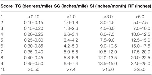
Table 1. Scoring scheme for variables RT, RS, SI, and RF.

Scores used from this table are divided by 10 and then substituted in the WI equation. Therefore, the feasible range for WI value varies between 0 and 1.0.

WI Model Validation

To test the ability of the WI model in forecasting weather conditions at a proposed EES site, the model was applied to a selected sample of existing weather stations that were treated as proposed new sites in Montana. Specifically, a total of 16 sites were selected from various regions in the state with different numbers of surrounding stations. First, a predicted WI was developed at those selected sites using weather information from surrounding stations only as well as weather predictions using published temperature and precipitation contour maps for the state of Montana. Then, the WI was calculated using actual weather information from the selected sites (referred to later as actual WI). The two values (predicted and actual) are compared and the percentage difference is determined. In this analysis, weights of WI model were selected using the researcher’s best judgment.

Validation results are shown in Table 2. The second and third columns show the calculated WI based on predicted and measured weather information, respectively. The fourth column in this table is of particular importance as it shows the absolute value of the difference between the predicted and actual weather indices expressed as a percentage. The last column in this table shows the number of surrounding weather stations used in WI calculation.

TABLE 2

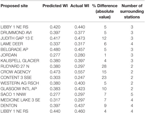
Table 2. Validation results of proposed weather index model.

The overall average difference between the predicted and actual WI is around 9% at all sites with the highest value being around 28%. The difference exceeded 10% at only four out of 16 sites, i.e., at 25% of the sites. A closer look at those sites clearly shows that the highest three values belong to sites that are surrounded by only two nearby weather stations that were used in WI calculations, and the fourth highest value at a site surrounded by three nearby stations. This observation implies a potential relationship between the accuracy of WI predictions and the number of surrounding weather stations used in WI calculations. To test this possibility, the relationship between percent difference and the number of surrounding stations was plotted and the best fit linear curve was established as shown in Figure 2. While observations are scattered, the general trend supports the tentative relationship, i.e., the more surrounding stations used in calculations, the less the difference between the predicted and actual WI. The coefficient of correlation was found to be −0.49, which is consistent with the assumed relationship and the trend shown in Figure 1.

FIGURE 1

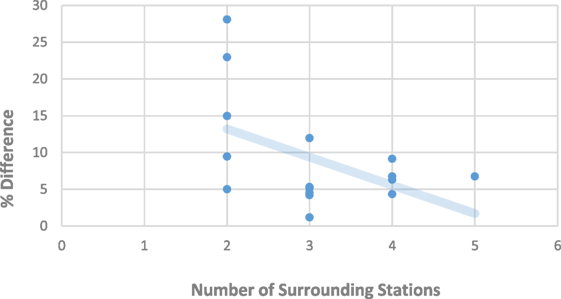
Figure 1. Percent difference versus number of surrounding stations.

FIGURE 2

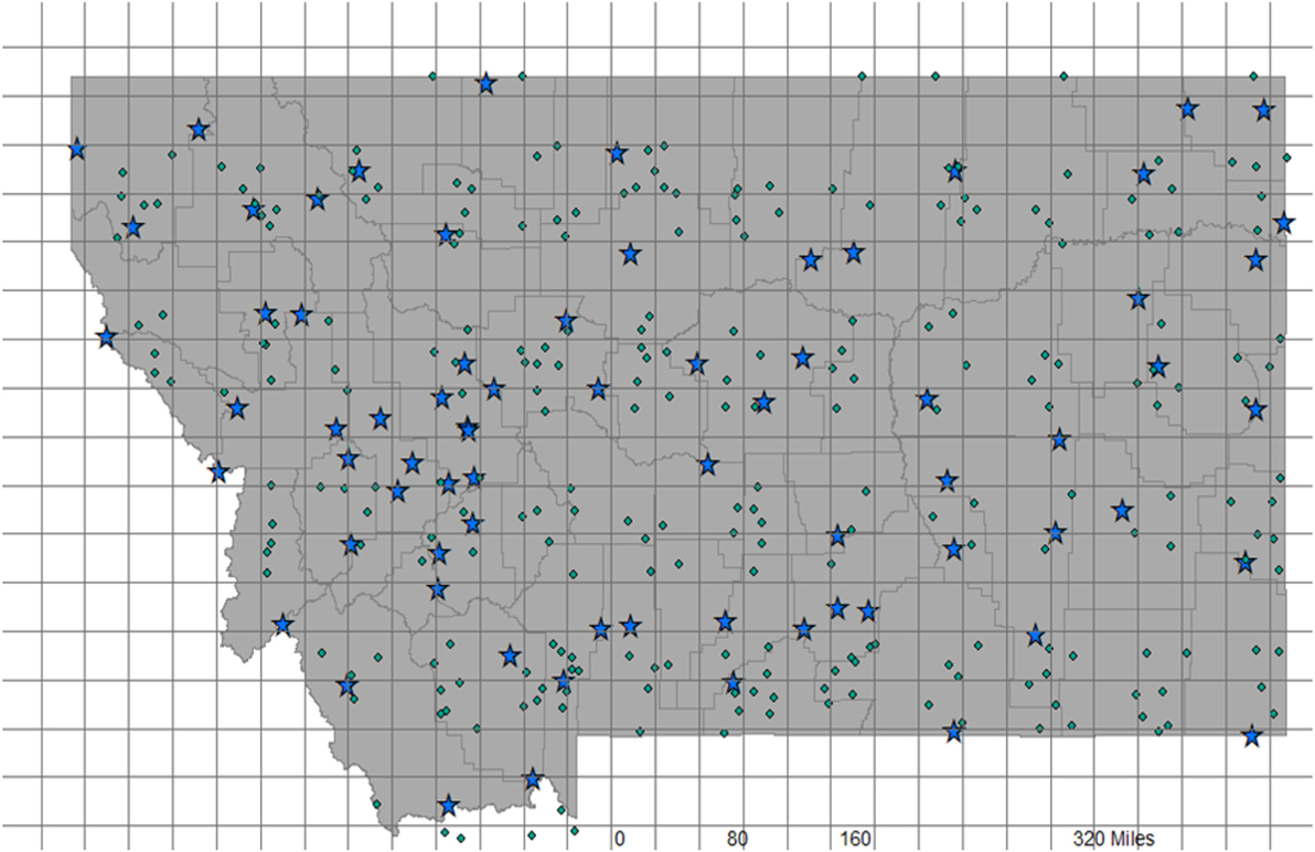
Figure 2. Weather stations in the state of Montana using 30 × 30 miles grid lines.

Traffic Index

A major consideration in the siting of a new ESS station is the amount of traffic that is expected to benefit from the weather information produced by the ESS station. In general, the amount of traffic is largely a function of the highway network surrounding the weather station and the functional class of highways in the network. The amount of travel expressed in million vehicle miles of travel (MVMT) within a 30-mile diameter circle around the proposed site was used to account for traffic variables. The amount of travel was calculated using the annual average daily traffic (AADT) and segment length for all highways in the network except local roads using the following equation:

$\mathrm{MVMT}=\frac{{{\displaystyle \sum }}_{i=1}^n({\text{AADT}}_i\ast 365\ast L_i)}{1,000,000}$

where AADT_i is the annual average daily traffic for segment i, L_i is the length of segment i, and n is the number of segments within the 30-mile circle surrounding proposed ESS site.

A scoring scheme for the amount of travel was developed using travel information for the state of Montana as shown in Table 3. This score will then be divided by 10 to find the TI to be used in the OM equation.

TABLE 3

Table 3. Amount of travel scoring scheme.

Crash Index (CI)

Another consideration in assessing the merit of a new ESS station is the safety of the route along which the proposed site is located. It is logical to expect that routes with high crash experience and particularly weather-related crashes to benefit more from weather information produced by a proposed ESS station.

In this research, crash rate per MVMT along 20-mile segment of the route where the proposed ESS station is located and the percentage of weather-related crashes are used in calculating the crash index. The aforementioned segment extends 10 miles upstream and 10 miles downstream of the proposed site. Crash severity is accounted for in calculating crash rate by using Equivalent Property Damage Only (EPDO) crashes where different weights are assigned to injury and fatal crashes based on the estimated crash cost of each severity of crash. Once all crashes are converted to EPDO crashes and using the AADT for all sections comprising the 20-mile segment route, crash rate (CR) can be calculated using the following equation.

$\text{CR}=\frac{C\ast 100,000,000}{{{\displaystyle \sum }}_{i=1}^{n}365\ast {\text{AADT}}_i\ast T\ast L_i}$

where C is the total number of EPDO crashes on the 20-mile evaluation segment, AADT_i is the annual average daily traffic for section i, T is the evaluation time period in years, L_i is the length of section i, and n is the number of sections in the 20-mile segment.

Using crash statistics in the state of Montana, a scoring scheme was developed for crash rate representing the crash experience along the route where the proposed ESS site is located. This scoring scheme is provided in Table 4.

TABLE 4

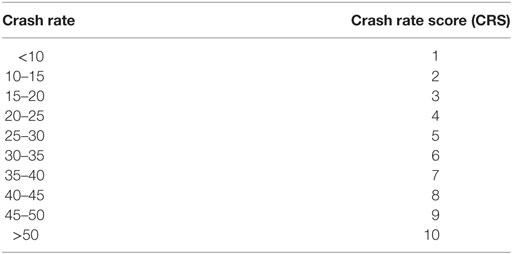
Table 4. Crash experience scoring scheme.

While crash history overall is important in assessing the merit of installing new ESS stations, weather-related crashes are of particular importance. To account for inclement weather risks along the route, the percentage of weather-related crashes (PW) is used along with crash rate score (CRS) in calculating the CI using the following equation:

$\mathrm{CI}=\mathrm{MIN}[1,(\text{CRS}/10)\ast (1+(\text{PW}-0.10))]$

where CI is the crash index, CRS is the crash rate score, and PW is the percentage of weather-related crashes to total crashes.

Other OF

As discussed earlier, the availability of power and communications infrastructure should add to the merit of a proposed ESS site, and the lack of power, communications or both should negatively affect the merit of a proposed site. While the availability of grid power at a proposed site is always a plus, the use of solar panels at isolated sites has widely been used and may provide an affordable alternative. In regard to communications, the lack of a wireless mobile network or telephone lines at the proposed site may require connecting the site using fiber optic cables, a solution that may prove to be costly. The OF scoring scheme developed consists of four different scenarios and associated scores as shown in Table 5. The score from this table should be divided by 10 when used in the OM formula.

TABLE 5

Table 5. Opportunistic factors (OF) scoring scheme.

Geographic Coverage of ESS Stations

Another aspect of assessing the merit of proposed ESS stations is the area coverage by existing weather stations. Specifically, areas and regions that have sparse weather stations may be good candidates for new ESS installations. Likewise, it may be somewhat difficult to justify a new ESS installation in areas where multiple weather stations exist. In this assessment, both RWIS and non-RWIS weather stations should be considered. However, the fact that RWIS stations are directly located along important routes while non-RWIS stations are usually located at some distance from surrounding highways, the two types should be treated differently.

To assess the geographic coverage of ESS stations in the proposed model, the state of Montana was divided into uniform units of area using a 30 × 30 miles grid, and weather station coverage was then established and expressed as the number of square miles per station, i.e., the larger the number the lower the coverage. Figure 2 shows weather stations in the state of Montana using the 30 × 30 miles grid lines. The stars refer to existing RWIS stations, while dots refer to other weather stations.

Each non-RWIS station was treated as 0.7 RWIS station in calculating coverage, given the higher utility expected from RWIS stations in supporting transportation applications. The area of a single grid unit (900 square miles) is then divided by the number of weather stations to determine coverage. Using data from the state of Montana shown in Figure 2 above, a scoring scheme from 1 to 5 was developed to assess the coverage at a particular proposed site (see Table 6 below). When using this variable in the OM model, the score from Table 6 should be divided by 5 for use in the model.

TABLE 6

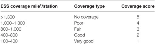
Table 6. Scoring scheme for environmental sensor station (ESS) coverage.

Application of Proposed Model

To demonstrate the application of the proposed ESS merit model, five hypothetical sites in the state of Montana were selected to represent different regions, highway class, and weather conditions. Information on selected sites from Montana Department of Transportation (MDT) records is provided in Table 7, and the location of sites on the state county map is shown in Figure 3.

TABLE 7

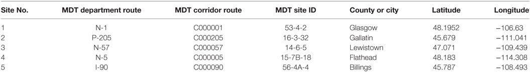
Table 7. Description of selected sites per Montana Department of Transportation (MDT) records.

FIGURE 3

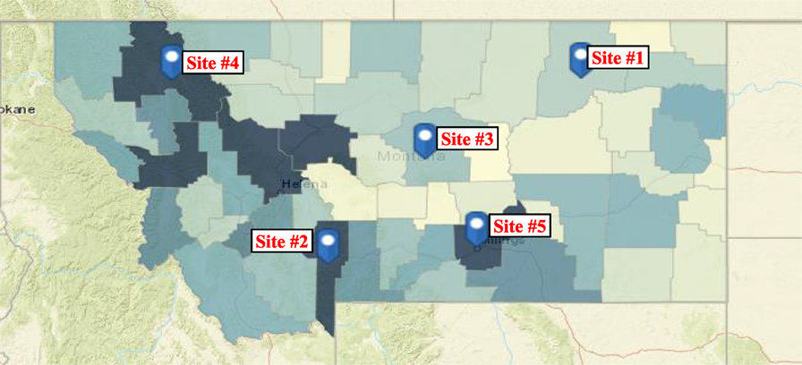
Figure 3. Selected sites on Montana county map.

Information on selected sites were gathered, variables were calculated using the equations and charts used in the proposed procedure, and the OM of sites were determined using the OM model. All sites were assumed to have access to grid power and mobile communication network. Equal weights (w₁ = w₂ = w₃ = w₄ = w₅ = 0.2) were used for model variables in this sample application. Results of the analysis are presented in Table 8.

TABLE 8

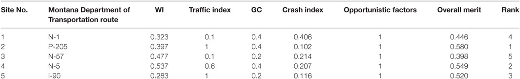
Table 8. Application of proposed model on selected sites.

As can be seen in Table 8 above, installing ESS station at site #2 is expected to provide most utility (benefits) followed by site # 4, site #5, site #1, and site #3, respectively.

Closing Remarks

The current paper presents a new model for prioritizing proposed ESS sites in a state or region by assessing the merits of those sites using weather, traffic, and safety data among other variables. Unlike most of the models proposed in the literature, the current model considers many variables that are thought to affect the merit (or need) of ESS installation while being more objective in assessing the contribution of those variables to the OM model.

Inputs to the proposed model include WI, TI, crash index, geographic coverage, and OF. The WI at a proposed site is determined using multiple indicators of weather severity and variability. The proposed crash index, another major input to the OM model, incorporates crash rate along the route and the percentage of weather-related crashes over the analysis period. The third input to the merit model, the TI, reflects the amount of travel on the highway network in the area surrounding the proposed ESS site. The fourth input to the merit model accounts for the ESS existing coverage in the area where the proposed site is located while the fifth and last input accounts for the availability and ease of access to power and communications. Model coefficients are represented by weights assigned to different model inputs that reflect the contribution of each input (variable) to the OM of the ESS site. Those weights are user-specified and should be selected to reflect the agency preferences and priorities.

A demonstration of the application of the proposed model using a selected sample of five sites in the state of Montana is presented to help readers understand the way the model could be used in practice.

Author Contributions

This research was part of a project funded by the Montana Department of Transportation (Project # 8229-001). AA-K was the principal investigator on this project while LE was the co-principal investigator where both authors worked closely in performing all project tasks.

Conflict of Interest Statement

The authors declare that the research was conducted in the absence of any commercial or financial relationships that could be construed as a potential conflict of interest.

Acknowledgments

The authors would like to acknowledge the financial support to this project by the Montana Department of Transportation (MDT) and the Federal Highway Administration (FHWA). The authors would also like to thank the project technical panel for their support and guidance throughout the project.

References

Hawkins, N., and Albrecht, C. (2014). Multi-Purpose ESS/ITS Data Collection Sites. Ames, IA: Aurora Program and FHWA.

Google Scholar

Jin, P., Walker, A., Cebelak, M., and Walton, M. (2014). Determining strategic locations for environmental sensor stations with weather-related crash data. Transp. Res. Rec. J. Transp. Res. Board 2440. doi: 10.3141/2440-05

CrossRef Full Text | Google Scholar

John, M., Walters, T., Wilke, G., Osborne, L., FHWA. (2005). Road Weather Information System – Environmental Sensor Station Siting Guidelines – Version 1.0. Washington, DC: Federal Highway Administration.

Google Scholar

Kwon, T., and Fu, L. (2013). Evaluation of alternative criteria for determining the optimal location of RWIS stations. J. Mod. Transp. 21, 17–27. doi:10.1007/s40534-013-0008-9

CrossRef Full Text | Google Scholar

Manfredi, J., Walters, T., Wilke, G., Osborne, L., Hart, R., Incrocci, T., et al. (2008). Road Weather Information System Environmental Sensor Station Siting Guidelines, Version 2.0. Washington, DC: FHWA-HOP-05-026 & FHWA-JPO-09-012 for US Department of Transportation.

Google Scholar

Pinet, M., and Bielkiewicz, B. (2009). “Alberta RWIS network expansion, winter risk assessment and priority list for advanced winter maintenance strategies,” in Annual Conference of the Transportation Association of Canada (Vancouver, British Columbia).

Google Scholar

Pinet, M., and Lo, A. (2003). “Development of a road weather information system network for Alberta’s National Highway System,” in Annual Conference of the Transportation Association of Canada (St. Johns, Newfoundland).

Google Scholar

Surface Transportation Weather Research Center. (2009). Analysis of Environmental Sensor Station Deployment Alternatives. Bismarck, ND: North Dakota Department of Transportation.

Google Scholar

Yang, C., and Regan, A. (2014). Methodology for the prioritization of environmental sensor station installation (case study of South Korea). Transport Policy 32, 53–59. doi:10.1016/j.tranpol.2013.12.012

CrossRef Full Text | Google Scholar

Zwahlen, H., Russ, A., and Vatan, S. (2003). Evaluation of ODOT Roadway/Weather Sensor Systems for Snow and Ice Removal Operations Part I: RWIS. Columbus, OH: FHWA/OH-2003/008A for Ohio Department of Transportation.

Google Scholar