Spatial–Temporal Analysis of the Heat and Electricity Demand of the Swiss Building Stock

Introduction

The global energy statistic report (BFE, 2016) and the sectorial energy consumption analysis of Kemmler et al. (2014) show that around 40% of the Swiss final energy consumption is used for space heating (SH) and domestic hot water (DHW) production. Adding the energy consumed by other building services to heat demand, shows that around half of the total final energy consumption can be attributed to the building sector. For this reason, the 2050 Swiss Energy Strategy targets to reduce the demand of the Swiss building stock by 63%, while increasing the share of renewable energy (Kirchner et al., 2012). The 2050 Swiss Energy Strategy has ambitious CO₂ emission reduction targets as well. Replacing fossil energy resources by electricity will raise questions on how to satisfy the increasing electricity demand (58 TWh in 2015).

Using Kaya’s identity, Mavromatidis et al. (2016) emphasize that reaching these targets will require to work along two axes: energy efficiency to reduce energy demand and substitution of fossil resources by renewables to reduce emissions per produced energy unit. A precondition to design strategies allowing to progress along these two axes is to have a better knowledge of the territorial energy demand. Territorial aspects related to heat and electricity consumption are a main concern of major EU research projects, such as Connolly et al. (2013), Persson et al. (2014), and David et al. (2017). The territorial aspect of heat demand is predominant, since heat is difficult and expensive to transport over long distances. Renewable heat resources are numerous but often linked to spatial–temporal constraints. For example, the use of high enthalpy geothermal and/or waste heat requires the development of district heating networks. At the Swiss national level, the potential use of these resources is studied by the SCCER FEEB&D (2017) project hosted by the Swiss Center of Competence in Energy Research (SCCER). The project is based on a spatial–temporal characterization of energy demand and renewable energy supply; one of its tasks is to design optimal decentralized energy systems that are able to match both the demand and supply side.

The characterization of heat and electricity consumption is also an important topic to better understand the effectiveness of energy efficiency programs. Heat demand reduction can be achieved, for example, by retrofitting the building envelope, using ventilation with heat recovery and improved building control systems. The effect of the performance gap, defined as the discrepancy between the expected and real savings achieved by building retrofit, was quantified by Khoury (2014) the for post-war multi-family residential buildings of the Canton of Geneva. How this gap impacts the projected heat demand reduction of the entire Swiss building stock is estimated in Section “Impact of Large-scale Retrofit on Heat Demand.” The design of programs that target the reduction of electricity demand is more complex because of the different possible uses of electricity. Detailed knowledge of how the electricity demand of a territory breaks down into various activities and electric appliances is a precondition for such a program. This is illustrated by Le Strat’s (Le Strat, 2008) study giving a detailed analysis of how electric consumption has evolved in the Canton of Geneva. In 2009, this study was used to redesign the large-scale electricity savings program ECO21 launched by the energy service company SIG. This knowledge allows, for example, to make ex ante estimations of savings achievable by large-scale electric device replacement, such as efficient lighting in the common areas of residential buildings. Expected versus actual savings for two ECO21 subprograms were compared (Cabrera et al., 2012) using three different approaches.

Geographical information systems (GIS) have gained major importance thanks to the increasing computing power and data storage capacities combined with big data analysis techniques. The use of GIS databases to assess energy demand and renewable resources is relevant at several territorial scales. Studies at the regional scale use building level demand as input for their models, as, for example, Saner et al. (2014) and Orehounig et al. (2014). The potential of combining thermal and PV solar panels is assessed for one urban and one suburban district by Quiquerez et al. (2015) using a GIS analysis. At the Swiss national scale Eicher et al. (2014) use GIS demand models aggregated on a hectare raster. At a much bigger scale, such as the European Union, Connolly et al. (2013) or Persson et al. (2014) use a 1-km² raster grid.

This paper presents two geo-dependent energy demand models, the first deals with final energy demand for SH and DHW production and the second one concerns electricity demand. The two following subsections give specific background information for these two models.

Geo-Dependent Heat Demand

The review paper of Swan and Ugursal (2009) outlines a clear classification of available models that estimate heat demand of buildings. Bottom-up models have the advantage that they estimate the energy demand of small consumer aggregates, as for example buildings that can be linked to geographical coordinates. To estimate the energy demand at the building level, the two main alternatives are to use either engineering or statistical models.

Engineering models are based on building physics and require detailed information on the building geometry as well as the envelope components and their associated U and g values. At the national scale such detailed data are not available and default values for many parameters must be used (Perez et al., 2011) when simulating the heat demand of a large building stock. Choosing this approach implies that buildings of same type have the same losses by conduction through the building envelope. Energy demand, therefore, only depends on local climate conditions and solar gains.

Statistical models encapsulate the complex set of building characteristics that explain the energy demand in a smaller set of parameters. Regression models estimate these parameters using calibration samples of buildings with known energy consumption. Another advantage of basing the model on measured energy demand is that it includes the influence of the users (inhabitants and facility manager). This influence often leads to a difference between calculated and actual consumption even in cases where the characteristics of the building are known in detail (De Wilde, 2014).

These reasons motivate the choice of a statistical extrapolation method based on measured final energy consumption; such a method accounts for the behavior of the user and the variability of demand between buildings with similar characteristics. A representative sample of around 27,000 buildings containing measured final energy for SH and DHW is used to calibrate the model.

Geo-Dependent Electricity Demand

There are numerous methods to simulate load curves. The review paper of Grandjean et al. (2012) classifies the most relevant algorithms into five groups, including both random (replicating the diversity of consecutive days) and deterministic models (replicating average behavior). For example, high-resolution models, such as Marszal-Pomianowska et al. (2016), seek to include the stochastic variability of electricity demand related to the behavior of the inhabitants. At the Swiss national level, the goal is rather to provide a large-scale model based on the average behavior of users and their related activities. The proposed approach is closer to that of the FORECAST/eLOAD model (Jakob et al., 2014). The primary target is to offer the Swiss municipalities a tool allowing to identify electricity saving potential and to predesign an ECO21 type program. The key question is how the electric demand of a municipality is divided into the various activities and electric appliances.

The model presented in Section “Geo-Dependent Electricity Demand” is the result of a collaboration between the academic research project SCCER FEEB&D (2017) and the local utility SIG. The basis for this model is a study of Le Strat (2011) that characterizes the electric consumption of a territory including all the energy service companies (ESCO) of the EOS holding group. This model decomposes the electricity demand into 36 activities and 18 groups of electric appliances. The planned outcome of this collaboration is the ElectroWhat web platform, which seeks to answer the question “who consumes where, when and for what use” at the national level. Throughout this paper, the term ElectroWhat often also refers to the geo-dependent electricity demand model.

Finally, the resulting GIS data of both models is stored in a database developed in collaboration with EPFL in Lausanne, also containing the renewable PV rooftop potential (Assouline et al., 2015) and low enthalpy geothermal potential (in preparation). Such a database offers the opportunity to perform many territorial studies at the Swiss national level.

Methods

This section describes the methods used to make a geo-dependent characterization of heat and electricity demand. These two demands are linked for buildings that are heated using electricity. In this case, we first start to estimate the final energy demand for SH and DHW using the heat demand model. For each municipality we use the fraction of dwellings that are equipped with electric heat production systems. For this fraction, the heat demand is then converted into electricity using efficiency factors that depend on the heat production system (resistance electric heating or heat pump). The yearly demand estimations are then divided in monthly demands using ratios of monthly degree day (DD) over yearly DD.

Geo-Dependent Heat Demand

The chosen approach, presented in this section, is a statistical regression bottom-up model (Schneider et al., 2016). It is based on measured heat demand and heated surfaces values of a representative set of around 27,000 buildings. It estimates the heat demand per square meter of each building of the Swiss national building register as a function of its category, age, and location, and its heated surface as a function of the category, gross surface, and/or dwelling surface. A bootstrap resampling algorithm quantifies the uncertainty inherent to the use of average demand values per age and category. This model improves previous work done by Eicher et al. (2011). Figure 1 outlines the general structure of the model. The heated surface A_E (square meter) and the floor specific heat demand E (MJ/m²/year) are estimated combining basic information provided by the Swiss building register (OFS, 2014a) with average statistics calculated using calibration sets. The estimations of the heated surface A_E and floor specific heat demand E are done separately, since they allow to take account of regional climate conditions that may vary a lot depending on geographical position. We assume that only E depends on climatic conditions, whereas the relation between A_E and gross building surface (A_gross) and/or dwelling surface (A_dwelling) do not. The final energy demand SE_B (MJ/year) of a building is obtained by multiplying these two estimations.

FIGURE 1

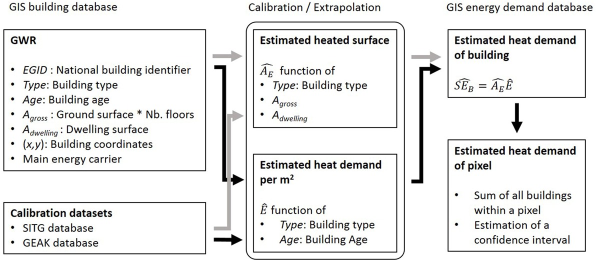
Figure 1. Heat demand model overview.

Finally, for each pixel of territory, the estimated heat demand is summed over all buildings and a bootstrap algorithm allows to compute a confidence interval around the estimated value given by the model.

Datasets

The model uses the following datasets:

(i) The Swiss national building register (GWR) maintained by the Swiss Federal Statistical Office (OFS, 2014a) that contains basic building information such as: geographical coordinates, category, age, ground, and dwelling surface as well as the main energy carrier for approximately two million buildings. This database is not exhaustive for non-residential buildings. A comparison with the Swiss building footprint data layer (Swiss Topo, 2015) shows that around 400,000 buildings are missing. A unique federal building identification number (EGID) identifies each building, which allows to link these data with other databases. Basic building information data, such as building category, construction period, A_gross, A_dwelling, geographical coordinates, and main energy carrier are extracted from this dataset.

(ii) The Geneva SITG IDC database contains measured energy consumption as well as heated surface A_E defined according to the SIA 416/1 standard for residential multi-family buildings and buildings used for non-residential purpose. This declaration is mandatory and is updated each year by a network of trained agents. This database (SITG, 2015) contains around 16,000 buildings, out of a total of approximately 48,000 buildings for the Canton of Geneva.

(iii) The GEAK database contains the energy consumption for SH and DHW averaged over 3 years. The database contains 11,500 buildings (approximately 0.5% of the Swiss building stock) spread over the entire Swiss territory.

(iv) The SIA 2028 standard (SIA, 2010) contains DD for 40 meteorological stations. Figure 2 displays the fit of a linear regression between the DD, altitude and latitude in CH_LV03 coordinates. Each dot of the scatterplot represents the estimated versus measured DD of a meteorological station. This linear fit will be used at later stage to estimate the DD for each building of the GWR using its altitude and geographical coordinates. The R² is 0.95, the maximum observed relative difference is 14% and the average difference is 4%.

FIGURE 2

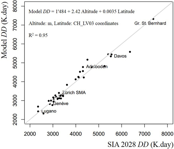
Figure 2. Model degree day DD versus SIA 2028 DD for all Swiss meteorological stations.

Estimation of Heated Surface A_E

Cross-matching the SITG IDC and GWR databases allows to study the relations between building category, gross surface, dwelling surface, and actual heated surface indicated in the SITG IDC database. Figure 3 shows such a linear regression for the multi-family residential buildings. The buildings with known heated surface A_E of the SITG IDC database are divided into four main categories and ten sub-categories based on a classification that divides the sample into groups with significant differences for the ratio A_E/A_gross. Table 1 gives the regression coefficients obtained from ten different building categories, given by 8,951 observations from the SITG IDC database. These regression coefficients allow to estimate for each building of the GWR database, the heated surface A_E by means of the gross surface (number of floors x ground surface) and/or the dwelling surface. If both estimations are possible, priority is given to the estimation based on gross surface because the coefficient of determination R² of the linear regression is higher.

FIGURE 3

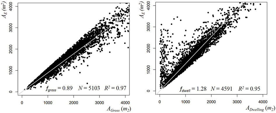
Figure 3. Heated floor area A_E as a function of gross surface A_gross and A_dwelling for multi-family buildings.

TABLE 1

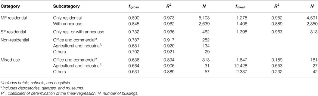
Table 1. Regression coefficients between heated floor surface and gross surface (f_gross) and between heated floor surface and dwelling surface (f_dwell), as observed in the IDC database.

Finally, for each building of the IDC database and for both linear regressions, we compute the relative error ΔA_E (%) between the actual and the estimated heated surface using

$\mathrm{\Delta }{A}_E=\frac{A_E-f_{\text{gross}}\cdot A_{\text{gross}}}{f_{\text{gross}}\cdot A_{\text{gross}}},$ (1)

$\mathrm{\Delta }{A}_E=\frac{A_E-f_{\text{dwell}}\cdot A_{\text{dwelling}}}{f_{\text{dwell}}\cdot A_{\text{dwelling}}}.$ (2)

These values, which are stored per building subcategory, will be used further down in Eq. 10 for the calculation of confidence intervals.

Note that the GEAK database, which is anonymous, could not be linked to the gross and dwelling surfaces of the GWR, reason why it is not used in this part of the calculation.

Heat Demand Estimation

For each building of the GWR database, the specific final energy for the heat demand SE_B is estimated by means of its age and category, using average values given by the SITG IDC and GEAK datasets, which are normalized to a common climatic reference. Due to its geographical specificities, Switzerland has important climatic differences between regions that depend mainly on altitude variations. To take this into account, a climatic correction is done to adapt the heat demand of a building to the local climatic conditions it is subject to.

Normalization of Calibration Data to a Common Reference

Since the heat demand data of the GEAK and SITG IDC calibration sets concern a variety of energy carriers and locations, it must first be normalized to a common reference. Therefore, for each building of these datasets, the measured final energy demand E (MJ/m² year) is converted into useful heat demand for SH using the relation

$Q_{\text{SH}}={\mathrm{\eta }}_{\text{EC}}E-Q_{\text{DHW}},$ (3)

η_EC (depending on energy carrier) is the transformation efficiency factor estimated by Khoury (2014) and Q_DHW the useful heat demand for DHW according to the SIA 380/1 norm. For buildings with thermal solar panels, Q_DHW only accounts for the fraction of the DHW demand which is produced by the main heat production system. In such a case, using $Q_{\text{DHW}}^{\text{SIA}}$ in Eq. 3 would lead to overestimating Q_DHW and underestimating Q_SH. To avoid underestimated Q_SH values the following constraint is added, which implies that at least one third of the total produced heat is used for SH

$Q_{\text{DHW}}=\min \left(Q_{\text{DHW}}^{\text{SIA}},2/3{\mathrm{\eta }}_{\text{EC}}E\right).$ (4)

This thumb rule sets an upper limit for the ratio between Q_DHW and Q_SH that corresponds to very efficient buildings. This limit is based on observations made in buildings with high energy standards for which the energy required for DHW can be higher than the one for SH. Note that this choice will have limited influence on the final result since it only impacts the fraction Q_SH of E that is subject to the climatic correction of Eq. 5 and only concerns a small fraction of buildings. The impact of this thumb rule was evaluated by looking at the difference between $\overline{Q_{\text{SH}}^{\text{GE}}}$ (see Eq. 7) calculated with the constraint (4) and $\overline{Q_{\text{SH}}^{\text{GE}}}$ calculated without. All absolute differences are below 2% and the average difference is 0.2% considering all categories and construction periods.

The useful energy demand values for SH are further normalized for each building to a common climatic reference (arbitrarily Geneva) using

$Q_{\text{SH}}^{\text{GE}}=Q_{\text{SH}}\frac{\text{DD}\left(\text{GE}\right)}{\text{DD}\left(\text{building}\right)},$ (5)

DD(building) stands for the standard SIA 2028 heating DDs of the climatic station associated to the building of the calibration set. The assumption behind this climatic correction is that the yearly demand for SH depends linearly on the DD. For this reason a ratio of DD between two climatic regions allows to estimate the Q_SH of a building in various climates.

Finally, the SITG IDC and GEAK data sets allow computing 15,588 and 11,499 $Q_{\text{SH}}^{\text{GE}}$ values normalized to the Geneva climatic reference.

Computing the DD for Each Building of the GWR

Combining the geographical coordinates with a topographic altitude model permits to compute the altitude of each building of the GWR using Eq. 6. Figure 2 illustrates the fit of the linear regression model estimating DD(building) by means of the building altitude Alt(building) and latitude Lat(building)

$\text{DD}\left(\text{building}\right)=1484+2.42\text{ Alt}\left(\text{building}\right)+0.0035\text{ Lat}\left(\text{building}\right).$ (6)

Statistical Analysis by Building Category and Age

For the purpose of statistical analysis, the previous data is grouped in four categories of buildings (multi-family residential, individual residential, non-residential, mixed use). For each of these categories, the data is further divided into 12 construction periods, and analyzed in terms of the statistical distribution of $Q_{\text{SH}}^{\text{GE}}$ as displayed in Figure 4. At this stage, it is worthwhile noticing that the variability within each construction period is much higher than between the periods, as previously observed by Khoury (2014). Note that this subdivision is different from the one used for the A_E estimation, since the building characteristics that influence the specific heat demand are not the same as those influencing the ratio between A_E and A_gross.

FIGURE 4

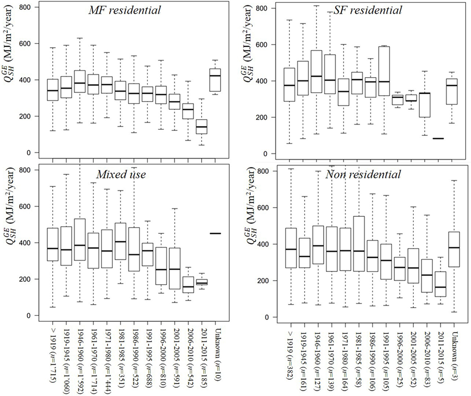
Figure 4. Boxplot distribution of $Q_{\text{SH}}^{\text{GE}}$ by construction period and building category (SITG IDC database).

Finally, for each building category and construction period, the average SH demand, which will be used for extrapolation of the GWR database is defined by

$\overline{Q_{\text{SH}}^{\text{GE}}}=\frac{{\sum }_{\left\{\right\}}{Q}_{\text{SH}}^{\text{GE}}{A}_E}{{\sum }_{\left\{\right\}}{A}_E}.$ (7)

The sum in Eq. 7 is made for all buildings of same category and construction period contained in the calibration samples. The average is weighted by A_E to give more importance to large buildings since they will also have more influence in the energy demand of a portion of territory. This will reduce the bias that could be introduced by small buildings having extreme specific heat demand $Q_{\text{SH}}^{\text{GE}}$.

This analysis is done separately for the SITG IDC and GEAK datasets, the respective values being used for the reconstruction of the entire GWR building stock located in Geneva, respectively, for the rest of Switzerland.

Heat Demand at Building and Pixel Levels

For each building of the GWR database, the final energy demand per square meter is estimated by the average demand of the corresponding category and construction period using

$\widehat{E}=\raisebox{1ex}{$1$}\!\left/ \!\raisebox{-1ex}{${\mathrm{\eta }}_{\text{EC}}$}\right.\left(\overline{Q_{\text{SH}}^{\text{GE}}}\frac{\text{DD}\left(\text{building}\right)}{\text{DD}\left(\text{GE}\right)}+Q_{\text{DHW}}\right)$ (8)

Since the average specific heat demand $\overline{Q_{\text{SH}}^{\text{GE}}}$ is normalized to the Geneva climate, it must then be adapted to the local climate conditions in which this estimation will be used. The DD ratio of Eq. 8—the inverse of the one of Eq. 5—transforms the Q_h of the Geneva climate into the ambient building climate. The DD(building) of the building is computed by using in Eq. 6 the geographical coordinates and the altitude of the building.

On this basis, the sum of the estimated heat demand of all buildings contained in a pixel of territory is computed using

${\widehat{\mathit{SE}}}_{\text{Pixel}}={\displaystyle \sum _{B\in \text{Pixel}}}\widehat{{\text{SE}}_B}={\displaystyle \sum _{B\in \text{Pixel}}}\widehat{A_E}\hat{E}.$ (9)

The upper procedure is repeated for the entire Swiss territory, for square pixels of scalable sizes, ranging from 100 m to 1.6 km.

Confidence Intervals

For each of the above pixels, we compute a confidence interval for the estimated heat demand value. It is computed using the bootstrap resampling algorithm (Efron and Tibshirani, 1993), which consists in generating a heat demand distribution replicating the dispersion of the calibration datasets. A random sampling within the sets of relative errors $\mathrm{\Delta }\widehat{A_E}$ defined by Eqs. 1 and 2 allows to replicate the error of the linear regression models used to estimate the heated surface A_E. A random sampling in the distribution of $Q_{\text{SH}}^{\text{GE}}$ values replicates the diversity of heat demand per square meter within a building category.

Finally, for each building of the pixel, a replicated ${Ê}^{\ast }$ value is generated by replacing the average $\overline{Q_{\text{SH}}^{\text{GE}}}$ value of Eq. 8 by a randomly picked value in the corresponding calibration dataset (same building category and construction period). Similarly, the heated surface $\widehat{A_E}$ is replaced by

${\widehat{A_E}}^{\ast }=\left(1+\mathrm{\Delta }\widehat{A_E}\right)\widehat{A_E},$ (10)

where $\mathrm{\Delta }\widehat{A_E}$ is a randomly picked relative error of the corresponding linear regression model. Feeding the ${Ê}^{\ast }$ and ${\widehat{A_E}}^{\ast }$ values into Eq. 9, generates a replicated heat demand for the entire pixel. Repeating this procedure a 1,000 times per pixel generates the heat demand distribution of each pixel. Finally, the limits of the 10% level confidence interval are the 5 and 95% percentiles of this distribution. Similarly, this distribution is used to calculate the 5 and 1% level confidence intervals.

Geo-Dependent Electricity Demand

This section describes the model used to decompose the electric demand of a territorial unit into various activities and groups of electric appliances (Schneider et al., 2017). The choice of a Swiss municipality is adequate since it represents the smallest political entity of Switzerland. For this reason many socioeconomic indicators are available at this level. In 2016, Switzerland had 2,287 municipalities of quite heterogeneous size. The number of residential dwellings ranges from 14 to 224,774, the city of Zürich being the biggest municipality after the city of Geneva. Since the spatial constraint for electricity is lower than for heat, it did not seem of interest to break down the territory into pixels as in the case of heat demand. Another particularity of certain regions is that the ratio between main and secondary residences varies a lot. The percentage of main residential dwellings ranges from 52% for the Canton of Graubünden to 98.8% for the Canton of Basel. This socio-economic characteristic has an important influence on energy demand.

As illustrated in Figure 5, the yearly demand of a municipality is split into three main sectors, each one with its own estimation algorithm as described in the following two subsections. The yearly consumption (YC) is split into 36 activities and 18 electric appliances such as lighting, fridges, TV, etc. A further step consists in transforming the yearly demand into estimated load curves using a library of load curve shapes.

FIGURE 5

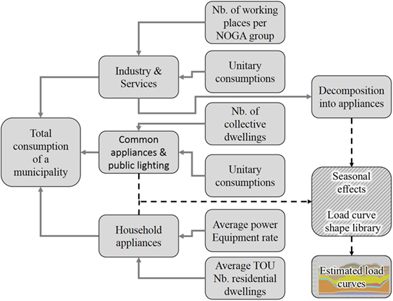
Figure 5. Overview of the geo-dependent electricity demand model.

The heat demand model of Section “Geo-Dependent Heat Demand” allows to estimate the final energy demand for SH and DHW. Combining these estimations with fractions of dwelling using electric heat production systems permits to estimate the amount of electricity used for SH and DHW. In case electric heat production is based on a heat pump, we use an average coefficient of performance of 2.5 to convert useful heat into electric demand.

Yearly Demand per Activity and Electric Appliance

Industry and Services

For each municipality, the estimation of the YC of the industry and services sector is based on the number of employees per NOGA activity code available in the STATENT database (OFS, 2014b). This statistic is combined with unitary average consumption per employe and NOGA code. For the territory of Geneva and of the EOSh group, these unitary consumptions are estimated using the total billed electricity per activity. For the remaining Swiss municipalities, the average unitary consumptions are calculated using a yearly national survey collected from approximately 12,000 companies (Bendel et al., 2011). This approach is similar to the one used by the FORECAST/eLOAD model (Jakob et al., 2014), with the difference that FORECAST/eLOAD uses profiles for occupancy and appliance distribution over time provided by the SIA Standard 2024 (SIA, 2015).

A next step consists in estimating for each NOGA activity code, the amount of electricity used for each group of electric appliances. This further distribution of the electric consumption is based on average fractions of the total electricity consumed by each group of electric appliances; these fractions come from audit and case studies. Finally, for each NOGA activity code these fractions allow to split up the total yearly demand into different appliances, as for example lighting, motor force, heat, etc. After completion of this step, the yearly estimated electricity consumption of the Industry and services sector is split into 55 activities and 15 electric appliances.

Common Appliances and Public Lighting

The common appliances of a collective residential building include the lighting of the staircase, the elevator, the common laundry, air ventilation and other technical installations. The size and age will of course have an influence on the consumption of these services. Nevertheless, for estimation on a large scale, average values representing an average sized building will be accurate enough. For public lighting the main underlying assumption is that the installed light power (including traffic lights) is linked to urban density. This approximation does not account for specificities, as for example extra urban highways and tunnels. These two kinds of electric consumption are supposed to depend mainly on the number of collective dwellings. Consumption is estimated by combining number of dwellings and unitary consumptions per dwelling.

As in the previous section, priority is given to unitary consumptions calibrated on local ESCO bills to account for regional differences. For example, there are big differences among several Swiss regions in use practices of lighting in the common areas of buildings. In Geneva, for example, it is mandatory to have the staircase illuminated day and night. The ECO21 program promotes low consumption light fixtures with occupancy sensors allowing the light to switch on only when required. In the Canton of Vaud, the common practice is to have staircase lighting with a manual switch.

The Residential Sector

The consumption of the average household is estimated by combining equipment rates, times of use and average power for each main use appliance. The unexplained part is included in the appliance “other.” A stock model, based on sales statistics of electric devices per energy efficiency label, permits to estimate the average power used by a device. Such sales statistics are available in the report (EAE, 2009), for example.

Several European norms define the efficiency of the device in terms of the electric consumption per unit according to the device type. For fridges (2003/66/CE), the label gives the ratio between the consumptions of the labeled device and a standard one. In this case, the normal consumption of the standard fridge depends mainly on the refrigerated volume.

The average YC of a device currently in operation is computed by summing the products of average consumption per efficiency label YC(E_Label) and the fraction of devices in operation

$\text{YC}={\displaystyle \sum _{\left(E_{\text{Label}}\right)}}\text{YC}\left(E_{\text{Label}}\right)F\left(E_{\text{Label}}\right).$ (11)

For most electric devices, the same average estimated YCs are used for the entire Swiss territory. The main regional difference concerns the equipment rate of electric cookers.

Estimation of Load Curves

A library of average load curve shapes per electric appliance type and activity permits to split the YC into monthly estimations. The used percentages defining these shapes are based on measured seasonal effects that are particularly pronounced for heating and lighting. Monthly demand is further broken down into daily demand for working and non-working days and finally into hourly demand. The load curve of a particular municipality is estimated by adding the individual load curves of all activities and all electric appliances.

GIS Energy Demand and Renewable Resources Database

Relational database servers and data exchange protocols, as for example the simple object access protocol (SOAP) are powerful tools allowing data interconnection originating from different sources. To facilitate data exchange, a database has been set-up in collaboration with EPFL that consolidates results of the geo-dependent energy supply and demand models. This consolidation fulfills the following requirements:

• Gives the results of our model estimations for energy supply and demand on a harmonized geographical aggregation level (municipality level and 200 m × 200 m pixel size).

• Displays documentation on the delivered data.

• Provides easy and flexible access to data using a web-service.

• Provides scripts allowing to build a part of this database (heat demand).

The actual release of the database contains rooftop PV potential (Assouline et al., 2017) with monthly and yearly values for each municipality in Switzerland as well as yearly heat demand and electricity estimations derived from the models presented in this paper. The database provides PV supply potential and heat demand estimations up to a resolution of 200 m × 200 m pixels. Concerning electricity demand, the database contains for each municipality the yearly demand estimation split up into activities and appliances. A dedicated web-service allows to query the database using the SOAP protocol. The user manual and sample of scripts to query the database are in the report of Schneider et al. (2015).

Results and Applications of the Models

The primary target of both models is to achieve a geo-dependent energy characterization of the Swiss energy demand. Nevertheless, it is of interest to derive some statistics aggregated at the national level and to compare them (as shown in Sections “Heat Demand Statistics Aggregated at the National Level” and “Validation of the Electricity Demand Model”) with other available statistics. This helps identifying potential biases of the models.

Sections “Heat Demand Maps,” “Impact of Large-scale Retrofit on Heat Demand,” and “Electricity Demand Maps and Web Platform” give some applications of the models, as for example drawing GIS maps and estimating possible potentials of reduction of demand linked to retrofit scenarios.

Heat Demand Statistics Aggregated at the National Level

Table 2 contains aggregated values—per building category and construction period—of the total heated surface A_E and final energy consumption for SH and DHW. Sufficient information is available to calculate these estimations for around 90% of the 1.93 million buildings listed in the 2013 version of the GWR. These values lead to a total heated surface estimation of 702 million m² and a total final energy demand of 93.7 TWh/year (76.8 TWh/year for residential and 16.9 TWh/year for mixed use and non-residential buildings). Within the residential sector 71% of the energy is consumed by buildings built before 1980. The fact that these buildings also have a high heat demand per square meter emphasizes the importance of thermal envelope retrofitting.

TABLE 2

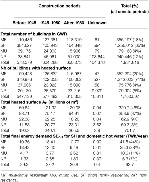
Table 2. Aggregated results of geo-dependent heat demand model.

Comparing these numbers with the estimation of an alternative study permits to detect a possible bias of the present model. For year 2013, Kemmler et al. (2014) estimate SE_CH to be 91.1 TWh/year, (59.5 TWh/year for residential and 31.6 TWh/year for mixed use and non-residential buildings). Although the two models have a good concordance for global demand, significant differences exist when considering the residential and non-residential sectors separately, mainly due to the differences between the estimated heated surfaces. In the case of the residential buildings, our model estimates a heated surface of 580 million square meter that is significantly higher than the one 509 million square meter estimated by Kemmler et al. (2014). This lower estimation would lead to a ratio f_dwell of 1.2 that is significantly lower than the value of Table 1.

Heat Demand Maps

Since the model delivers energy demand estimation at the building level, Eq. 9 permits to compute the aggregated demand for pixels of any size. Dividing the Swiss territory into a raster of pixels and exporting, pixel by pixel, the demand to an information system such as QGIS, allows us to draw heat demand maps. Figure 6 gives an example of such a heat density map for Switzerland, with a zoom on the town of Martigny. A color ramp indicates the final energy consumption per square meter of territory for each pixel of 200 m × 200 m size. Such maps permit to identify portions of territory having high demand density, being consequently suitable for district heating deployment. Cross-matching these demand maps with other geo-referred information, as for example availability of waste heat, permits to estimate the exploitation potential of such resources. Other information, as for instance, the percentage of demand covered by fossil energy carriers can be added to derive estimated CO₂ emission maps.

FIGURE 6

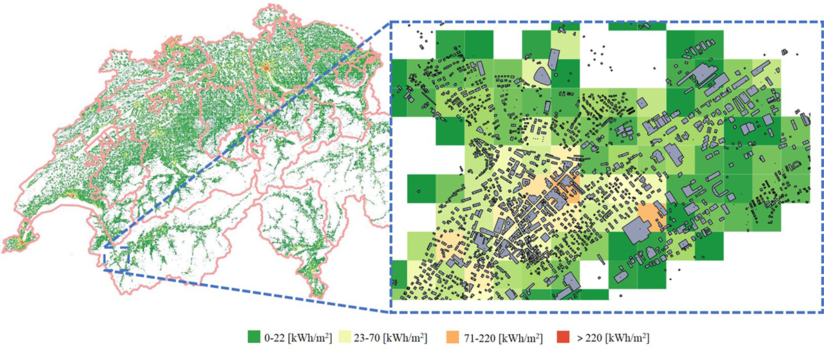
Figure 6. Swiss geographical information system map for heat demand and zoom on the town of Martigny.

Impact of Large-scale Retrofit on Heat Demand

The previously presented geo-dependent heat demand database allows estimating the savings that could be achieved by large-scale retrofit of building envelope. The new energy policy scenario (NEP) of the Swiss Energy Strategy 2050 targets reducing today final energy demand for SH and DHW production to around 42 TWh/year; this represents a decrease of 53%. This section challenges this scenario by making the optimistic assumption that today retrofit rate will double to reach 2%. If current retrofit practices are applied, the SIA 380 standard (SIA, 2009) sets an upper limit Q_SH,lim (MJ/m²) for the calculated useful energy demand per square meter. This demand is calculated under normed conditions for indoor temperature and ventilation rate that are not often fulfilled in real use conditions after retrofit. This discrepancy between the normed and real use of the building induces a performance gap. This gap is the difference between the theoretical savings QS_Gross (MJ/m²) defined by

${\mathit{QS}}_{\text{Gross}}=Q_{\text{SH}}-Q_{\text{SH,lim}},$ (12)

and the actual savings QS_Net (MJ/m²) defined by

${\mathit{QS}}_{\text{Net}}=Q_{\text{SH}}-Q_{\text{SH\_AR}},$ (13)

where Q_SH,AR is the actual measured energy demand per square meter after retrofit. The analysis of ten representative case studies (Khoury et al., 2016) of recently retrofitted post-war multi-family residential buildings allowed to characterize the performance gap by means of a statistical correlation between QS_Gross and QS_Net

${\mathit{QS}}_{\text{Net}}=0.0009{\left({\mathit{QS}}_{\text{Gross}}\right)}^2+0.17{\mathit{QS}}_{\text{Gross}}\text{if}{\mathit{QS}}_{\text{Gross}}<600\text{MJ}/{\text{m}}^2.$ (14)

This relation (R² = 0.9897) takes account of the entire retrofit process, from the design stage (choice of solutions and use of simulation software) to the use of the buildings by the occupants and energy managers. It can be viewed as a characterization of the current retrofit and operation practices. In case QS_Gross exceeds 600, we use the more conservative value QS_Net = 0.7 QS_Gross. This rule applies to buildings having a theoretical energy savings that lies outside the range of the building sample analyzed by Khoury et al. (2016).

The analysis of this section will show that taking account of the performance gap has a significant effect on the savings of large-scale retrofit programs. Figure 7 shows the procedure used to estimate the net saving potential of a group of buildings that are supposed to be retrofitted in accordance with the efficiency limit of the SIA 380 standard. We start by assigning to each of these buildings a shape factor, which is defined as the ratio between the building thermal envelope surface A_th and its heated surface A_E. These ratios are taken from the SIA 2031 standard (SIA, 2016) for all the building categories, except for the multi-family residential buildings. For the latter, the factors are estimated on the basis of the number of floors using the relation below, which was derived from the GEAK database.

$\raisebox{1ex}{$A_{\text{th}}$}\!\left/ \!\raisebox{-1ex}{$A_E$}\right.=0.32+\raisebox{1ex}{$1.97$}\!\left/ \!\raisebox{-1ex}{$\sqrt{N_{\text{floors}}}$}\right..$ (15)

FIGURE 7

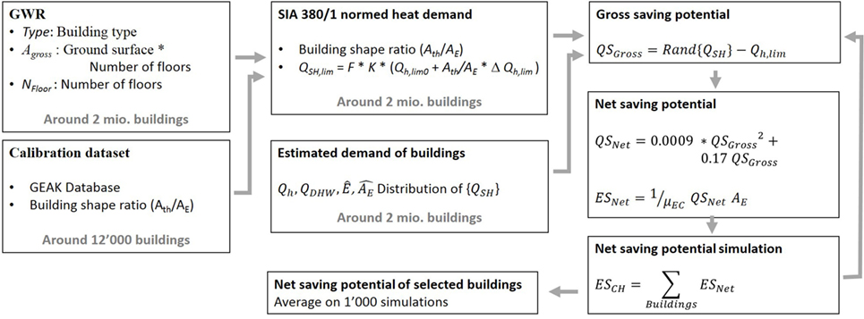
Figure 7. Estimation of gross and net energy saving potential after retrofit of a building group.

These shape factors permit to compute for all buildings the limit value Q_SH,lim, which is the heat per square meter demand a building should not exceed after retrofit. The heat demand of the building for SH before retrofit is estimated by a randomly picked Q_SH value taken from our calibration set of buildings of same category and construction period (see Eq. 5). This randomization replicates the variability of the observed distribution of heat demand of buildings of same category. Using an average value instead of this distribution would not have any effect on the average QS_Gross value, but would bias the QS_Net estimation, because of the quadratic term of Eq. 14. Putting these two values into Eq. 12 allows to estimate the gross saving potential per square meter QS_Gross for each building. Eq. 14 allows to compute the net saving potential per square meter that is then converted into final energy using Eq. 16.

${\mathit{ES}}_{\text{Net}}=\raisebox{1ex}{$1$}\!\left/ \!\raisebox{-1ex}{${\mathrm{\eta }}_{\text{EC}}$}\right.{\mathit{QS}}_{\text{Net}}{A}_E.$ (16)

Finally, to compute the total net savings $E{S}_{\text{Net}}^{\text{CH}}$, we sum the net saving potential ES_Net of all buildings supposed to be retrofitted. This procedure is repeated 1,000 times and the average of the $E{S}_{\text{Net}}^{\text{CH}}$ values gives the net saving potential of the retrofitted building group.

For future projections concerning the building stock size and the evolution of its energy demand, we refer to the report of Prognos (Kirchner et al., 2012). This study expects an increase of heated surface of 32% between 2010 and 2050. In the present simulation, it was supposed that all new buildings added to the current building stock consume 100 MJ/m²/y of final energy for SH and DHW.

Figure 8 shows how the possible evolution of the final energy demand for 2020, 2035, and 2050 using the previously explained estimation procedure. Under the assumption no retrofit is done, the total demand SE_CH will increase proportionally less than the additional heated surface, since the new buildings are supposed to be very efficient. The doted gray lines are the expected evolution of demand according to the new energy policy scenario (NEP) and business as usual scenario (WWB) of the 2050 Swiss energy strategy. In our 2% per year retrofit rate scenario, it is assumed that the buildings offering the highest saving potential are retrofitted first. Even following this optimistic assumption the expected savings $E{S}_{\text{Net}}^{\text{CH}}$ are significantly lower than the projection given by the WWB scenario. Disregarding the performance gap leads to savings $E{S}_{\text{Gross}}^{\text{CH}}$ that are close to the projections of Prognos.

FIGURE 8

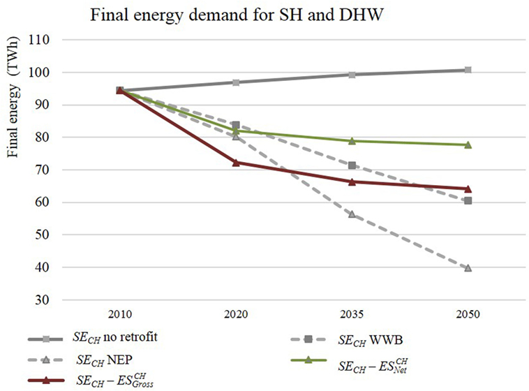
Figure 8. Evolution of final energy demand of the Swiss building stock for SH and domestic hot water (DHW).

Validation of the Electricity Demand Model

This section presents two kinds of validations done by comparing estimates obtained from the model with available electricity consumption statistics. A first validation consists in comparing estimated and actual annual consumptions at the national and at different regional levels. This enables to check the accuracy of the unitary consumptions used to estimate the YCs in the various sectors of activity. A second validation compares the estimated hourly demand with the measured one. The way the model builds the estimated hourly load curve implies that load curves are identical for all the days of the same month and day type (working, non-working). It is thus adequate to compare the estimated load curve with the average load computed by taking separately working and non-working days for each month and hour of the day. This kind of comparison checks if the shapes of the load curve library and the weights used for aggregation replicate actual demand.

Validation of Annual Consumptions

The annual consumptions are compared at the national, cantonal and municipality levels. Table 3 compares for the year 2008 estimated electricity consumptions and alternative statistics from several sources. As explained in Section “Yearly Demand per Activity and Electric Appliance,” the estimations of the model give priority to unitary consumptions calibrated on local ESCO bills to take account of regional differences. If such data are not available for the region of interest, average Swiss default values are used. For this reason, the accuracy of the model depends on the level of available information.

TABLE 3

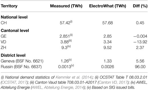
Table 3. Comparison of aggregated yearly demand estimations with other data sources.

At the national level, the report of Kemmler et al. (2014) provides yearly estimations for the main sectors of activity. At this aggregation level there is a very good match showing that the used average Swiss unitary consumptions per activity do not introduce a bias at this level.

Certain cantonal energy offices publish electricity consumption statistics on their home pages. The calibration values of the model for the Canton of Geneva are based on bills issued by the local utility SIG. Therefore, the cantonal aggregated estimated consumption is very close to the actual consumption. For the two other examples of Cantons, bigger differences are observed. The estimation for the Canton of Zurich uses Swiss average default values for all unitary consumptions, since no statistics for unitary consumption per activity are available for this region.

The collaboration with SIG has allowed to access almost all electricity bills of the Canton of Geneva. Comparing actual and estimated electricity demand for each municipality of the Canton Geneva permits to check how accurate the estimation remains when used for smaller territorial units. Figure 9 plots estimated versus billed electricity demand for the 44 municipalities of the Canton. For the Canton of Geneva, the average difference between actual and estimated demand of a municipality is 16%, with differences ranging from 0.6% (Aire-la-Ville) to 96% (Russin).

FIGURE 9

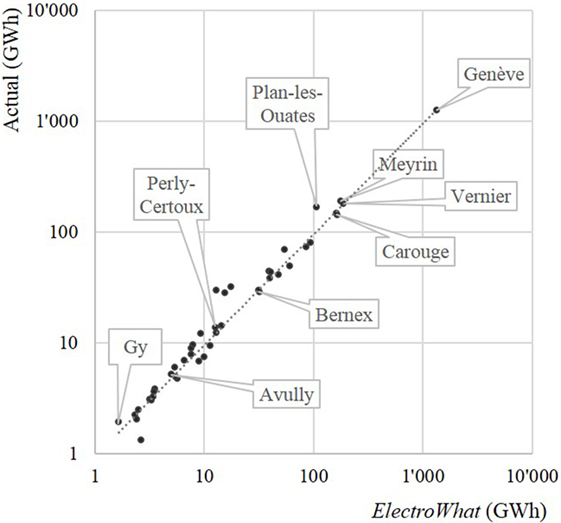
Figure 9. Actual versus estimated electricity consumption for the year 2008 of the 44 municipalities of the Canton of Geneva.

Validation of Load Curve Profiles

This section compares the estimated load curve with two measured load curves; the first aggregated at the level of the Canton of Geneva and the second at the level of Switzerland. The comparison is done by comparing for each month the estimated and actual load curve representative of an average day. Taking separately for each hour the average demand of all days of the same month permits to compute a load curve representative of an average day. Since a large part of the demand is due to the industry and services sector, working and non-working days are considered separately.

Figure 10 displays for each month (1–12 on the x-axis) the average daily load curve in black and the simulated one in gray. The increase of demand in the cold winter months is quite limited since Geneva has almost no electric heating. The simulation replicates the daily shape quite well with morning (11 a.m.) and evening peaks (7 p.m.) due to cooking as well as lighting appliances in the evening. The evening peak is greater due to earlier sunset during winter. For week-ends, the overall load is less because the activity in the services and industry sector is lower; however, the evening peak induced by households becomes more obvious, especially during winter.

FIGURE 10

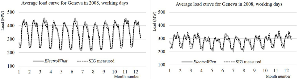
Figure 10. Actual and simulated average hourly load curve from January (1) to December (12) 2008 for the Canton of Geneva.

Figure 11 gives the same comparison for the Swiss overall load curve. The measured hourly load curve is estimated by SFOE (2009) every third Wednesday of each month. It is based on a consolidation of the net production (taking account of imports and exports) of all Swiss electricity producers. An estimated loss of 12% due to transportation and distribution was removed to reflect the final energy used by the end consumer. The main differences are seen for June and July where the model significantly overestimates the demand. At the Swiss level, around 10% of the SH and DHW production (Schneider et al., 2016) is covered by electricity. This explains a seasonal variability with higher demand during the winter months.

FIGURE 11

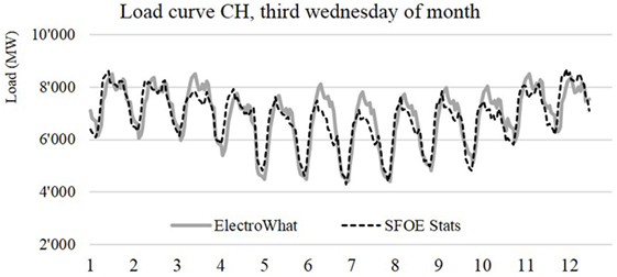
Figure 11. Actual and simulated average hourly load curve from January (1) to December (12) 2008 for Switzerland.

Electricity Demand Maps and Web Platform

Figure 12 shows an example of a GIS map combining yearly demand per capita, distribution of demand into four main activity sectors and total demand for some municipalities near the city of Lausanne. A quite high heterogeneity exists among the shares consumed per sector, also influencing the per capita consumption. In the municipalities of Aclens and Mex a large part of the demand is attributable to the services and industry sector, which induces a high demand per capita compared to a residential municipality such as Bussigny. This difference of socio-economic structure influences the distribution of demand into electric appliances and the shape of the load curve.

FIGURE 12

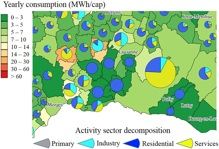
Figure 12. Example of electricity consumption map in the surroundings of the city of Lausanne.

The Electowhat model is used to set-up a prototype web platform allowing to explore the consumption specificities of each Swiss municipality. A report containing the main indicators is enriched with charts illustrating the distribution of the yearly demand into activities and electric appliances. This detailed distribution of electric consumption can be downloaded in Excel format for further treatment. A future step will be to include on this platform the experience gained by SIG during the implementation and monitoring of their electricity efficiency program ECO21. The platform will use the decomposed electricity demand provided by the model to help the user to design an efficiency program of ECO21 type in any region of Switzerland.

Discussion

Geo-Dependent Heat Demand

The geo-dependent heat demand model presented in Section “Geo-Dependent Heat Demand” is an alternative to commonly used calculation models based on building physics, which suffer from a lack of accuracy when used at large territorial scale, due to the limited available information on the building characteristics. Calibrating the model using measured final energy consumption bears the advantage of replicating the difference in energy demand between buildings with very similar characteristics. An innovative approach consists in using a bootstrap algorithm to compute a confidence interval in addition to the estimated demand of a pixel of territory. These confidence intervals quantify the part of variability the model cannot reproduce, when the specific heat demand Q_h of a building is replaced by the average demand of the buildings of same category and age.

There are two important assumptions linked to this kind of approach. The first is that the GWR database contains the majority of the heated buildings of Switzerland. The second is that the samples used to calibrate the bottom-up model are representative. Important deviations from these assumptions would introduce bias in the estimations. One possibility to detect bias is to compare, for example, the aggregate demand of all buildings with other available national scale statistics. As shown in Section “Heat Demand Statistics Aggregated at the National Level,” the total aggregated final energy demand for heating is 93.7 TWh/year (76.8 TWh/year for residential and 16.9 TWh/year for mixed use and non-residential buildings). Total demand is in good agreement with an alternative estimation based on national statistics, but significant differences exist when considering the demand of residential and non-residential sectors separately. The main cause for this discrepancy is the differences between the estimations of heated surfaces. Since the f_dwell values of Table 1 are based on a large number of observations, we are quite confident with our larger heated surface estimations for the residential sector. The alternative estimation used for comparison also comes from a model, which is subject to its own uncertainties.

The actual consumption data for buildings contained in the SITG IDC database allows to identify 206 pixels of 200 m × 200 m with known total final energy demand. Estimated demand together with its confidence interval and actual demand are compared for each of these pixels to test the accuracy of the bootstrap algorithm. For three chosen confidence levels α = 10, 5, and 1%, the proportion of pixels having their actual energy demand value outside the confidence interval are 15.5, 8.3, and 2.4%, respectively. The fact that these proportions are close to α, show the adequacy of the bootstrap algorithm.

Since retrofit has a major role to play in reducing demand and achieving the goals of the 2050 energy strategy of the Swiss Federal council, it is interesting to challenge the projections made by Prognos (Kirchner et al., 2012). Section “Impact of Large-scale Retrofit on Heat Demand” gives an example of how the heat demand model can be used to estimate the achievable heat demand saving potential of the Swiss building stock. For this sake, we relied on previous results (Khoury et al., 2016) concerning the performance gap between the gross and net heat demand savings achieved by building retrofit, which reflects the current retrofit and operation practices. When applying the results of the above mentioned study to our model, we estimate that if the entire Swiss building stock undergoes deep energy retrofit, the gross saving potential for SH would amount to 38.1 TWh/year. When taking into account the performance gap, the net saving potential for SH reduces to 18.4 TWh/year, i.e., almost half of the gross saving potential. A similar ratio between net and gross saving potential was already observed at a smaller scale in the canton of Geneva. Comparing projected savings for years 2020, 2035, and 2050 with the goals of the energy strategy 2050, we see that even when making optimistic assumptions on retrofit rate and selection of buildings, the net estimated savings remain far from the anticipated targets. This result is based on the assumption that the relation between net and gross saving potential applies to all building categories. Even if the projection of Figure 8 deserves deeper investigation, this first approximation already raises interesting questions. The projections of Prognos do not take into account the performance gap and may for this reason be too optimistic.

The approach given here has some limitations that are due to data availability. For instance, having an exhaustive GWR register would answer questions concerning possibly missing heated surface. A larger calibration set uniformly covering the entire Swiss territory and all building categories would also increase the accuracy of the model, as well as reducing the size of the confidence intervals.

Geo-Dependent Electricity Demand

The accuracy of the geo-dependent electricity demand model strongly depends on the detail level of the data available to calibrate the unitary consumptions per activity. This is illustrated in Table 3 that compares the estimated versus actual total aggregated demand for Cantons where local demand data was available—or not—for calibration. In the case of the Canton of Geneva, detailed consumption per activity is known, leading to representative unitary consumption of this region. In the Canton of Zurich, average Swiss values are used based on national energy consumption surveys for various activities. Although these default values lead to an unbiased estimation at the national level, they cannot replicate in detail the variability that energy demand may have between different regions, within the same activity. This phenomenon is also observed on a smaller scale, as shown in Figure 9, showing the errors at the level of each municipality, even when the model is calibrated with accurate Cantonal unitary consumptions. This reflects the fact that electricity demand within a same group of activities has a quite high variance that a large-scale model cannot reproduce.

A second type of validation compares estimated and actual load curves to check if the aggregation of the individual estimated load curves per activity and electric appliance lead to an overall demand, which is close to the average demand of a representative working and non-working day. Again, the added value of having local calibration data available is highlighted by the fact that the model replicates more accurately the demand of the Canton of Geneva than the overall national demand. Unlike the algorithm used for the FORECAST/eLOAD platform, no adaptations are done after the comparison. In our case the validation only serves to check if the load curve library and the weights used to combine the individual load curves reflect the average actual demand. Making further adaptations based on least square difference minimization may lead to completely biased coefficients since the number of degrees of freedom of the model is larger than the number of measured observations. We choose to let the model rely on parameters based on case study measurements and time of use model estimations for household appliances, without making any a posteriori adjustments.

It is interesting to observe that the fraction of heat production covered by electricity varies considerably according to the considered region (from 1% for Basel up to 25% for Vallis). This has an effect on the seasonal variation of the electric load curve of the region under consideration. The canton of Geneva has, for example, only a small fraction of electric heating (around 5% of total final energy). Consequently, the seasonal effect is less marked on Figure 10 than in Figure 11, since other regions of Switzerland have higher shares of electric heat production systems.

Conclusion

Specific approaches are used to estimate geo-dependent heat and electricity demand due to the variety of goals. In the case of heat demand, emphasis is placed on the spatial aspect because heat is more difficult to transport. Modeling electricity demand is more complex, since electricity has many possible uses. To decompose electricity demand per activity and per electric appliances in addition to the spatial characterization provides a big added value. It gives the base input to design electricity efficiency programs considering regional specificities. Further conclusions are given separately for the geo-dependent heat and electricity demand.

Geo-Dependent Heat Demand

The proposed bottom-up model operates at the building level and allows heat demand estimations for every geographical aggregation level. It is calibrated using large sets of measured final energy demand. This data was used to compute heat demand statistics per building category and construction period. Basing the model on measured consumptions has the advantage of including the influence of the user. In addition, this approach allows to estimate confidence intervals by means of a bootstrap resampling algorithm. The aggregated overall demand for the entire Swiss territory is in good agreement with national statistics, speaking in favor of the model.

A first outcome of the model is to build a database providing the heat demand for a pixel grid of the entire Swiss territory. As second possible use of the model, is the estimation of expected savings achievable through retrofit (see “Impact of Large-scale Retrofit on Heat Demand”). It is interesting to notice that taking account of the performance gap significantly reduces the projected savings (of approximately 50%). This kind of observation was already pointed out by Khoury (2014) in his study on multi-family residential buildings of the Canton of Geneva. Such discrepancies reveal key questions on some of the energy savings projections made for the 2050 energy strategy of the Swiss Federal council.

Geo-Dependent Electricity Demand

The used model breaks down the total estimated electricity demand of a municipality into estimated hourly load curves per activity and electric appliance. The University of Geneva, in collaboration with the local utility SIG, is currently updating the model in view of simulating the year 2015. The model—today calibrated using the year 2008—replicates well the average behavior at large-scale, but of course cannot replicate all local specificities. This is a consequence of the fact that the chosen groups of activities have some heterogeneity concerning the consumption per employee. For example, consider the activity “manufacture of machines and tools,” for which the energy intensity varies a lot depending on the type of manufactured good. Some regions might be more specialized in one or the other type of good, having consequently differences of consumption per employee. The consequence of using Swiss average values for large portions of the Swiss territory is that a part of the variability of demand remains unexplained, as seen in Table 3 and in Figure 9.

The comparison of aggregated estimated load curves with actual ones shows that the model replicates the most important seasonal and intraday variations. The present simulation can be done for any geographical level for which the required input variables reflecting socioeconomic activity and building stock are available. By default, the municipality level should be used, since it is the smallest geographical unit having all the required input information easily available at the national scale. This model also opens the perspective of making ex ante estimations of savings that could be achieved by standard efficiency measure packages. To this end, in collaboration with the SIG, it is planned to set-up a web-platform helping the user to design an efficiency program similar to ECO21 in any region of Switzerland.

Finally, the results of the geo-dependent heat and electricity models are consolidated with geo-dependent renewable resource data. This database is shared with other research partners and serves as base input to assess energy transition scenarios. Between 2018 and 2020, the second phase of the SCCER FEEB&D project (SCCER FEEB&D, 2017) will explore how to find the best trade-off between energy efficiency (building retrofit, ECO21 type programs, etc.) and use of renewable resources (PV, geothermal, heat pumps, waste heat, free-cooling, etc.). Such models combined with a consolidated database are the foundation for exploring energy transition pathways and deriving policy recommendations.

Nomenclature

Abbreviations
ECO21	Large-scale energy efficiency program launched in 2007 by SIG
EGID	Federal building identification number
ESCO	Energy service company
DHW	Domestic hot water
GEAK	Cantonal building energy certificate
GIS	Geographical information system
GWR	Swiss national building register maintained by the Swiss Federal Statistical Office
NOGA	General classification of economic activities, providing a numeric code per activity
SH	Space heating
SIG	Geneva’s energy service company Services Industriels de Genève
SITG IDC	Territorial information system of Geneva’s territory, index of heat consumption layer
SOAP	Simple object access protocol
Latin symbols
AE	Heated surface or energy reference surface defined by standard SIA 416/1 (m2)
Adwelling	Total surface of all residential dwelling of a buildings (m2)
Agross	Gross building surface as ground surface multiplied by the number of floors (m2)
Ath	Surface of the building thermal envelope (m2)
ΔAE	Relative error between estimated and actual AE (-)
DD(l)	Degree day of geographical location l (Kůday)
E	Final energy demand per m2 for SH and DHW production (MJ/m2/year)
ESNet	Net final energy saving potential for SH after retrofit (MJ/year)
F(L)	Fraction of electric devices actually in operation having efficiency label L (%)
g	Solar energy transmittance of glass windows (%)
QSH	Useful energy demand per m2 for SH (MJ/m2/year)
QSH,lim	Upper limit of calculated useful energy demand per m2 for SH according to standard SIA 380/1 (MJ/m2/year)
QSH,AR	Useful energy demand per m2 for SH after retrofit (MJ/m2/year)
QDHW	Useful energy demand per m2 for DHW (MJ/m2/year)
QSGross	Gross useful energy saving potential per m2 for SH after retrofit (MJ/m2/year)
QSNet	Net useful energy saving potential per m2 for SH after retrofit (MJ/m2/year)
U	Thermal transmittance of a building’s envelope component (W/m2ůK)
SEB	Final energy for SH and DHW production for a building (MJ/year)
SECH	Final energy for SH and DHW production for the Swiss building stock (TWh/year)
$\overline{X}$	Average value of variable X. For example $\overline{Q_{\text{SH}}}$ is the average useful energy demand for SH of a given building category
$\widehat{X}$	Estimated value of variable X. For example $\widehat{E}$ is the estimated final energy demand for SH and DHW production
YC	Yearly electric consumption of an electric device (kWh/year)
Greek symbols
ηEC	Efficiency of energy conversion system

Author Contributions

SS and PH are the main contributors of the methods described in section “Geo-Dependent Heat Demand.” JK and BL contribute to section “Impact of Large-scale Retrofit on Heat Demand.” PS and SS are the main contributors of the methods described in section “Geo-Dependent Electricity Demand.” MP provided the access to the GEAK database. SS wrote the manuscript.

Conflict of Interest Statement

The author declares that the research was conducted in the absence of any commercial or financial relationships that could be construed as a potential conflict of interest.

Acknowledgments

This research is part of the activities of SCCER FEEB&D, which is financially supported by the Swiss Commission for Technology and Innovation (CTI). The authors thanks the Swiss Federal Statistical Office for the free access to the GWR database.

References

Assouline, D., Mohajeri, N., and Scartezzini, J.-L. (2015). A Machine Learning Methodology for Estimating Roof-top Photovoltaic Solar Energy Potential in Switzerland. doi:10.5075/epfl-cisbat2015-555-560

CrossRef Full Text | Google Scholar

Assouline, D., Mohajeri, N., and Scartezzini, J.-L. (2017). Quantifying rooftop photovoltaic solar energy potential: a machine learning approach. Solar Energy 141, 278–296. doi:10.1016/j.solener.2016.11.045

CrossRef Full Text | Google Scholar

AWEL, Abteilung Energie. (2014). Energieplanungsbericht 2013, Bericht Des Regierungsrats Über Die Energieplanung Des Kantons Zürich. Zürich: AWEL, Abteilung Energie. Available at: www.energie.zh.ch

Google Scholar

Bendel, R., Brunner, F., and Ferster, M. (2011). Energieverbrauch in Der Industrie Und Im Dienstleistungssektor, Resultate 2010. Helbling Beratung + Bauplanung AG.

Google Scholar

BFE. (2016). Statistique Globale Suisse De L’énergie 2015. Bern: Bundesamt für Energie.

Google Scholar

Cabrera, D., Seal, T., Bertholet, J.-L., Lachal, B., and Jeanneret, C. (2012). Evaluation of energy efficiency program in Geneva: evaluation methodology and experience feedback for two subprograms using bottom-up approach. Energy Effic. 5, 87–96. doi:10.1007/s12053-011-9110-1

CrossRef Full Text | Google Scholar

Canton, VD. (2017). “Statistique Vaud,” in Estimation De La Consommation Finale D’énergie, Par Agent Énergétique, En TJ, Vaud, 1996–2015. Available at: http://www.scris.vd.ch/Default.aspx?DocID=1197&DomId=2211

Google Scholar

Connolly, D., Lund, H., Mathiesen, B. V., Werner, S., Möller, B., Persson, U., et al. (2013). Heat roadmap Europe: combining district heating with heat savings to decarbonise the EU energy system. Energy Policy 65, 475–489. doi:10.1016/j.enpol.2013.10.035

CrossRef Full Text | Google Scholar

David, A., Mathiesen, B. V., Averfalk, H., Werner, S., and Lund, H. (2017). Heat roadmap Europe: large-scale electric heat pumps in district heating systems. Energies 10, 578. doi:10.3390/en10040578

CrossRef Full Text | Google Scholar

De Wilde, P. (2014). The gap between predicted and measured energy performance of buildings: a framework for investigation. Autom. Constr. 41, 40–49. doi:10.1016/j.autcon.2014.02.009

CrossRef Full Text | Google Scholar

EAE. (2009). Verkaufszahlenbasierte Energieeffizienzanalyse Von ElektrogerätenSI/40017. Energie agentur electrogeräte(EAE). Available at: https://www.eae-geraete.ch/effizienzanalyse/

Google Scholar

Efron, B., and Tibshirani, R. (1993). An Introduction to the Bootstrap. Monographs on Statistics and Applied Probability 57. New York: Chapman & Hall.

Google Scholar

Eicher, H., Pauli, H., Erb, M., and Gutzwiller, S. (2011). Ausbau Von WKK in Der Schweiz WKK-Standortevaluation Auf Basis Einer GIS-Analyse. Liestal: Dr. Eicher+Pauli AG planer für Energie und Gebäude Technik.

Google Scholar

Eicher, H., Pauli, H., Sres, A., and Nussbaumer, B. (2014). Weissbuch Fernwärme Schweiz – VFS Strategie, Langfristperspektiven Für Erneuerbare Und Energieeffiziente Nah- Und Fernwärme in Der Schweiz. Liestal: Dr. Eicher+Pauli AG planer für Energie und Gebäude Technik.

Google Scholar

Grandjean, A., Adnot, J., and Binet, G. (2012). A review and an analysis of the residential electric load curve models. Renew. Sustain. Energ. Rev. 16, 6539–6565. doi:10.1016/j.rser.2012.08.013

CrossRef Full Text | Google Scholar

Jakob, M., Kallio, S., and Bossmann, T. (2014). “Generating Electricity Demand-Side Load Profiles of the Tertiary Sector for Selected European Countries,” in Proceedings of 8th International Conference Improving Energy Efficiency in Commercial Buildings (IEECB’14), Frankfurt. doi:10.2790/32838

CrossRef Full Text | Google Scholar

Kemmler, A., Piégsa, A., Ley, A., Wüthrich, P., Keller, M., Jakob, M., et al. (2014). Analyse Des Schweizerischen Energieverbrauchs 2000–2013 Nach Verwendungszwecken. Bern: Bundesamt für Energie.

Google Scholar

Khoury, J. (2014). Rénovation Énergétique Des Bâtiments Résidentiels Collectifs: État Des Lieux, Retours D’expérience Et Potentiels Du Parc Genevois. Université de Genève, thèse de doctorat No 4752, direction Bernard Lachal. Available at: http://archive-ouverte.unige.ch/unige:48085

Google Scholar

Khoury, J., Hollmuller, P., and Lachal, B. M. (2016). “Energy performance gap in building retrofit: characterization and effect on the energy saving potential,” in 19. Status-Seminar (Zurich: ETHZ). Available at: http://archive-ouverte.unige.ch/unige:86086

Google Scholar

Kirchner, A., Bredow, D., and Ess, F. (2012). Die Energie Perpectiven Für Die Schweiz by 2050. Basel: Prognos AG.

Google Scholar

Le Strat, P. (2008). Analyse De La Demande D’électricité Du Canton De Genève499 937 605 00016. Bures sur Yvette, France: Action énergies.

Google Scholar

Le Strat, P. (2011). Programme EOSh De Maîtrise De La Demande d’Electricité517 421 202 00014. La Baule, France: APOGEE.

Google Scholar

Marszal-Pomianowska, A., Heiselberg, P., and Kalyanova Larsen, O. (2016). Household electricity demand profiles – a high-resolution load model to facilitate modelling of energy flexible buildings. Energy 103, 487–501. doi:10.1016/j.energy.2016.02.159

CrossRef Full Text | Google Scholar

Mavromatidis, G., Orehounig, K., Richner, P., and Carmeliet, J. (2016). A strategy for reducing CO₂ emissions from buildings with the Kaya identity – a Swiss energy system analysis and a case study. Energy Policy 88, 343–354. doi:10.1016/j.enpol.2015.10.037

CrossRef Full Text | Google Scholar

OCSTAT. (2017). Statistiques Cantonales Genève (OCSTAT). Statistiques Cantonales, Electricité. Available at: http://www.ge.ch/statistique/domaines/08/08_02/tableaux.asp#3

Google Scholar

OFS. (2014a). Eidgenössisches Gebäude- Und Wohnungsregister,Web Services,Technisches Dossier Zum Datenaustausch via WebServices. Neuchâtel: Bundesamt für Statistik BFS.

Google Scholar

OFS. (2014b). Erhebungen, Quellen – Unternehmensstatistik (STATENT). Office fédérals de la Statistique. Available at: http://www.bfs.admin.ch/bfs/portal/de/index/infothek/erhebungen__quellen/blank/blank/statent/01.html

Google Scholar

Orehounig, K., Mavromatidis, G., Evins, R., Dorer, V., and Carmeliet, J. (2014). Towards an energy sustainable community: an energy system analysis for a village in Switzerland. Energy Build. 84, 277–286. doi:10.1016/j.enbuild.2014.08.012

CrossRef Full Text | Google Scholar

Perez, D., Kämpf, J. H., Wilke, U., Papadopoulou, M., and Robinson, D. (2011). “CitySimsimulation: the case study of Alt-Wiedikon, a neighbourhood of Zürich city,” in Proceedings of CISBAT 2011 – CleanTech for Sustainable Buildings, Lausanne.

Google Scholar

Persson, U., Möller, B., and Werner, S. (2014). Heat roadmap Europe: identifying strategic heat synergy regions. Energy Policy 74, 663–681. doi:10.1016/j.enpol.2014.07.015

CrossRef Full Text | Google Scholar

Quiquerez, L., Faessler, J., Lachal, B. M., Mermoud, F., and Hollmuller, P. (2015). GIS Methodology and Case Study Regarding Assessment of the Solar Potential at Territorial Level: PV or Thermal? Aalborg University Press. Available at: https://wwws.aau.dk/index.php/sepm/article/view/1043

Google Scholar

Saner, D., Vadenbo, C., Steubing, B., and Hellweg, S. (2014). Regionalized LCA-based optimization of building energy supply: method and case study for a Swiss municipality. Environ. Sci. Technol. 48, 7651–7659. doi:10.1021/es500151q

PubMed Abstract | CrossRef Full Text | Google Scholar

SCCER FEEB&D. (2017). SCCER Future Energy Efficient Buildings & Districts. Available at: https://www.sccer-feebd.ch/

Google Scholar

Schneider, S., Assouline, D., Mohajeri, N., and Scartezzini, J.-L. (2015). Geo-Dependent Energy Demand and Supply Web-Service. Available at: http://wisesccer1.unige.ch/

Google Scholar

Schneider, S., Khoury, J., Lachal, B., and Hollmuller, P. (2016). “Geo-dependent heat demand model of the Swiss building stock,” in Sustainable Built Environment Regional Conference. SBE 2016, 17th Edn (Zurich: SBE). Available at: https://archive-ouverte.unige.ch/unige:84240.

Google Scholar

Schneider, S., Le Strat, P., and Patel, M. (2017). “Electro what: a platform for territorial analysis of the electricity consumption,” in Proceedings of CISBAT 2017, Lausanne, Switzerland: EPFL. doi:10.1016/j.egypro.2017.07.376

CrossRef Full Text | Google Scholar

SFOE. (2009). Schweizerische Elektrizitätsstatistik 2008 Report: 805.005.08.d. Ittigen.

Google Scholar

SIA. (2009). Norme SIA 380/1:2009. L’énergie Thermique Dans Le Bâtiment. Zurich: Société suisse des ingénieurs et des architectes (SIA).

Google Scholar

SIA. (2010). Norme SIA 2028: Données Climatiques Pour La Physique Du Bâtiment, L’énergie Et Les Installations Du Bâtiment. Zurich: Société suisse des ingénieurs et des architectes.

Google Scholar

SIA. (2015). Norme SIA 2024: Données D’utilisation Des Locaux Pour L’énergie Et Les Installations Du Bâtiment. Zurich: Société suisse des ingénieurs et des architectes.

Google Scholar

SIA. (2016). Norme SIA 2031: Certificat Énergétique Des Bâtiments. Zurich: Société suisse des ingénieurs et des architectes.

Google Scholar

SITG. (2015). SITG Indice De Dépense De Chaleur (IDC) Des Bâtiments (LEn > 5.8.2010) – Moyenne Sur 2 Ou 3 Ans. Available at: http://ge.ch/sitg/sitg_catalog/sitg_donnees/i?keyword=IDC

Google Scholar

Swan, L. G., and Ugursal, V. I. (2009). Modeling of end-use energy consumption in the residential sector: a review of modeling techniques. Renew. Sustain. Energ. Rev. 13, 1819–1835. doi:10.1016/j.rser.2008.09.033

CrossRef Full Text | Google Scholar

Swiss Topo. (2015). Swiss Topo Topographic Landscape Model TLM. Available at: https://www.swisstopo.admin.ch/de/wissen-fakten/topografisches-landschaftsmodell.html

Google Scholar