Improving the Estimation of Markov Transition Probabilities Using Mechanistic-Empirical Models

Introduction

Many state-of-the-art infrastructure management systems are making use of the Markov model for the prediction of deterioration and the determination of the optimal intervention strategies. When using the Markov model, elements of infrastructures are considered to be in discrete states (deterioration condition states) defined using physical characteristics, and the deterioration of elements over time is described as probable transitions between these states over time.

In estimating transition probabilities, there are two basic situations, (1) there are sufficient time-series data, i.e., when sufficient data are available for a minimum of two consecutive time intervals and (2) there are no sufficient time-series data, i.e., when there are no sufficient data available for a minimum of two consecutive time intervals. Needless to say, infrastructure managers should make decisions of interventions for all elements by reliable transition probabilities when the management system uses Markov models. In the first situation, infrastructure managers use statistical methods to estimate the transition probabilities of the Markov models. Many of the models were developed with the assumption that elements could jump no more than one state per time period, such as those used in Klein (1962), Carnahan et al. (1987), Jiang et al. (1988), Madanat and Ben-Akiva (1994), and Thompson et al. (1998). However, others were developed without this assumption, such as those developed by Tsuda et al. (2006) and Kobayashi et al. (2012a,b). The former have the advantage that they are relatively easy to compute. In the former, however, as the deterioration being predicted is relatively rapid with respect to the time periods selected, error becomes non-negligible. For example, if it is assumed that the transition probability from state i to i + 2 in 5 years is 0, the model cannot express rapid deterioration processes. The latter allow to avoid this assumption and have the advantage that resulting transition probabilities lead to more accurate prediction of deterioration. In addition, they can be used when data have been collected at non-uniform intervals.

Despite progressive development in the field of monitoring over the last decades so that data can be collected more frequently and more accurately, the second situation likely occurs in municipalities with relatively small scale and it can be readily imagined that not a few administrative organizations are facing this situation. They are especially pertinent in developing nations, in which there is too little attention paid to managing infrastructures, including a vast number of concrete bridges. Situations such as (1) time-series data cannot be used to estimate the transition probabilities because historical intervention records between inspections are unavailable, (2) time series data are not recorded as electronic data, and (3) time-series data in current criteria of states are not available because criteria of states had been changed recently, come under this situation as well. In the situation where there are no sufficient time-series data, infrastructure managers either rely solely on expert opinion or use expert opinion in conjunction with predictions made using mechanistic-empirical models.

In mechanistic-empirical models, deterioration processes are modeled as physical processes that can be described using the characteristics and properties of the materials of the elements and their chemical and physical response/reaction against factors of the environment. Using mechanistic-empirical models, once the values of endogenous and exogenous factors governing the deterioration process are determined, the condition evolution of the bridge element over time can be estimated without the need for inspection data for a minimum of two consecutive time intervals. Unlike Markov models, condition evolution over time is modeled as being continuous (DuraCrete, 1998; Kirkpatricka et al., 2002). When mechanistic-empirical models are used together with expert opinion, it is usually assumed that an element cannot transition more than one state in one time period.

An improvement to the estimation of transition probabilities to be used in infrastructure management systems, and, therefore, an improvement to infrastructure management, would be to have a methodology to be used to estimate transition probabilities using mechanistic-empirical models for use in the second situation. In addition, it is desired that elements are modeled so that they can transition more than one state in one time period. Such a methodology is proposed in this article. The proposed methodology makes use of two approaches: (1) the analytical approach and (2) the Bayesian approach. The first is used in situations where it is possible to find an analytical solution so that the transition probability can be derived directly from the mechanistic-empirical models. The second is used in situations where it is not possible to find the analytical solution. It makes use of Bayesian statistics, which requires the formulation of a likelihood function of the transition probabilities and the use of Markov Chain Monte Carlo (MCMC) simulation.

The remainder of the article is structured as follows: Sections “Finite State Markov Models and Transition Probabilities” and “Estimating Transition Probabilities Using Mechanistic-Empirical Models” include a background to position the contribution of the proposed method. Specifically Section “Finite State Markov Models and Transition Probabilities” contains an overview of finite state Markov models and transition probabilities, and Section “Estimating Transition Probabilities Using Mechanistic-Empirical Models” contains a literature review regarding methods to estimate transition probabilities using mechanistic-empirical models. Section “Mechanistic-Empirical Models” includes the mechanistic-empirical models to be used in the work presented in this article. In the Section “Relationship between Mechanistic-Empirical Models and Transition Probabilities,” it is explained how transition probabilities are to be estimated analytically using mechanistic-empirical models. In Section “Methodology,” the methodology is described, in which, the steps to formulate the mechanistic-empirical model of deterioration process is given along with a way to convert the condition evolution predicted using this model to the discrete states required by the Markov model. An example of how the method is to be used is given in Section “Example.” In Section “Comparison with the State-of-the-Art,” the Markov models developed using the proposed methodology and a state-of-the-art methodology are compared. In the Section “The Number of Deterioration Paths from the Mechanistic-Empirical Models,” the effect of the number of deterioration paths required to obtain a satisfactory result is shown and discussed. Section “Conclusion” contains the conclusions of the work and recommendations for future research.

Finite State Markov Models and Transition Probabilities

In finite state Markov models, transition of condition states between time point t₁ and t₂ = t₁ + z is expressed with a transition probability matrix whose i* j (i = 1, …, I;j = 1, …, I) element is a transition probability defined as Prob[h(t₂) = j|h(t₁) = i] = π_ij. h(t) is a function which denotes a condition state at t. π_ij is a conditional probability which indicates the occurrence probability of condition state j at t₂ with given condition state i observed at t₁. In finite state Markov models, it is assumed that the transition probability between time points t₁ and t₂ is only dependent on the condition state at t₁ so as to satisfy the Markov property. Finite state Markov models have been used in the management of deteriorating systems since the 1960s, when there was a rapid development of mechanical and electrical systems (Howard, 1960; Gertsbakh, 2000; Kolowrocki, 2014). They have been used to ensure that to determine optimal intervention strategies, i.e., the strategy to follow to ensure that the costs of executing interventions are balanced with the costs of not executing interventions. Finite state Markov models allowed for the modeling of deterioration processes that could not be perfectly modeled deterministically, to be modeled as stochastic processes. They were, and are, considered to be good models for systems where the transitions from one state to another can be considered to be memoryless. They are less good where this is not the case but are still often used due to both their ease of use and ease of understanding in situations where the assumptions of memoryless do not lead to large deviations in condition evolution prediction from reality. To ensure that a Markov model is developed to give accurate predictions of deterioration using statistical methods, condition state data are required. In general, the longer the time series of inspections, the better.

Finite state Markov models are used in infrastructure management systems to model the deterioration of elements and to determine optimal intervention strategies (AASHTO, 2004; Swei et al., 2015). They are used instead of continuous Markov models due to their convenience, in terms of using visual inspections (it is easier to say that an element is in state 2 than to say if it is in 2.1, 2.2, or 2.3) and in terms of assessing the state of the element that is to trigger an intervention (Howard, 1960; White, 1992; Puterman, 1994). The estimation of the transition probabilities for the Markov models is ideally done using available condition state data that have been collected at uniform time intervals over a long period of time (Lee, 1970). Although somewhat more complicated, when data have been collected at non-uniform intervals of time over a long period of time, the transition probabilities can be estimated using statistical methods, such as survival analysis, maximum likelihood estimation, and Bayesian estimation approaches (Hastings, 1970; Lancaster, 1990; Kobayashi et al., 2012a; Mizutani et al., 2013; Lethanh et al., 2015). When little to no condition state data are available, transition probabilities have been estimated using expert opinion or estimated in various ways to obtain a best fit with the condition states predicted using mechanistic-empirical models (Golroo and Tighe, 2012; Indiana Department of Transportation, 2013).

To simplify the estimation of transition probabilities some researchers and developers of management systems have assumed that it is not possible for an element to move more than one condition state in one time interval, e.g., Jiang et al. (1988), Mishalani and Madanat (2002), and Robelin and Madanat (2007). However, others have explicitly developed models where that is not the case (Tsuda et al., 2006). Being able to estimate transition probabilities with data that have been collected at both uniform and non-uniform time intervals and allowing elements to move more than one condition state per time interval, it has been shown to increase the accuracy of the estimation of the transition probabilities in Markov models (Tsuda et al., 2006; Kobayashi et al., 2012b; Mizutani et al., 2013; Lethanh et al., 2015).

Estimating Transition Probabilities Using Mechanistic-Empirical Models

In situations where there are little to no time-series condition state data estimating transition probabilities so that the results of a Markov model fit those of mechanistic-empirical models, using mechanistic-empirical models is likely to yield more accurate deterioration predictions.

However, fitting can be done in different ways. No research has been conducted using an approach to find an analytical solution so that the transition probability can be derived directly from the mechanistic-empirical models. When this approach is unavailable due to relatively complicated functional forms of the mechanistic-empirical models, an approach is available to estimate the transition probabilities using the predictions of condition of the elements with the Markov model and with the mechanistic-empirical models. Roelfstra et al. (2004), which is perhaps the first work in this area, used a restricted least squares approach to minimize the difference between the predictions of the average condition of the elements with the Markov model and the predictions of condition of the elements with the mechanistic-empirical models. They assumed that there was a maximum transition of one state in one time interval. Overcoming this assumption, Lethanh et al. (2017) used a restricted least squares approach to minimize the difference between the prediction of the probabilities of the elements being in each condition state in each time interval within the investigated time period estimated using the Markov model and those predicted using the mechanistic-empirical models. In other words, they minimized the sum of the differences between the elements of the state vectors, which are estimated using the Markov model and the mechanistic-empirical models, respectively. In this process, however, information of the transitions of the states in each element, i.e., information of the transitions from state i to j of an element, is lost by aggregating this information into the values of the state vectors. To prevent this loss of information, in the proposed methodology, a likelihood function of the transitions of the states in each element is formulated, and the transition probabilities are estimated based on the likelihood function. The methodology used by Lethanh et al. (2017) is used as a reference methodology in this article.

Mechanistic-Empirical Models

Many mechanistic-empirical models can be used to predict the future condition state of reinforced concrete elements. In this work, a mechanistic-empirical model was selected to predict condition states of the element during the initiation phase of chloride-induced corrosion, and another was selected to predict condition states of the element during the propagation phase. The models used were based on those given in DuraCrete (2000). An illustration of the two phases, along with the ranges of chloride concentrations (kg/m³) and crack widths (mm) used to define the condition states, is given in Figure 1.

FIGURE 1

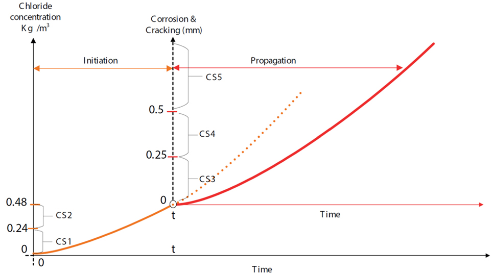
Figure 1. Deterioration process of reinforced concrete due to chloride-induced corrosion [adopted from Lethanh et al. (2017)].

Chloride penetration was modeled using Fick’s second law of diffusion (Fick, 1855).

$\frac{\mathrm{\delta }{C}_{\text{cl}}}{\mathrm{\delta }t}=D_{\text{cl}}\frac{{\mathrm{\delta }}^2{C}_{\text{cl}}}{\mathrm{\delta }{x}^2},$ (1)

where C_cl is the chloride ion concentration at the depth of the reinforcement (here small notation “cl” denotes the abbreviation for chloride); x is the depth; and D_cl is the chloride diffusion coefficient.

The solution for partial differential equation (Eq. 1) gives the following explicit form to calculate the chloride concentration as a function of the distance of the reinforcement from the concrete surface x_cl and time t (DuraCrete, 2000).

$C_{\text{cl}}\left(x_{\text{cl}},t\right)=C_s\left(1-\text{erf}\left[\frac{x_{\text{cl}}}{2\sqrt{D_{\text{cl}}t}}\right]\right),$ (2)

where C_s is the surface chloride content and erf[⋅] denotes the error function.

The time required for corrosion to start, that is time t in Eq. 2 was estimated by setting the value of C_cl to be equal to the chloride concentration. Then the value of C_cl is used to determine the entry point into a condition state. In other words, by setting the upper bounds on the values of C_cl to be used to define each discrete condition state i, the time to arrive at that condition state was obtained by solving Eq. 2 with respect to time t and a certain depth of concrete cover from the reinforcement. The value of variables C_cl, C_s, and D_cl in the above equations were considered to be random, with each one being represented with a probabilistic distribution.

After the value of chloride concentration reached a certain lower limit, corrosion of the reinforcement was assumed to start. After it reached a certain higher limit, cracking was assumed to start. The following equations from DuraCrete (2000) were used:

$w\left(t\right)=w_0+\mathrm{\beta }\left(P\left(t\right)-P_0\right),$ (3)

where w(t) is the crack width (mm) over time; β is the parameter that controls the propagation; w₀ is the crack width when it is visible (≈0.05 mm); P₀ is the amount of loss of re-bar diameter (mm) when the crack width is visible; and P(t) is the amount of loss of re-bar diameter (mm) at time t, which is given by the following equation:

$P\left(t\right)={\int }_0^t{V}_{\text{corr}}\cdot \mathrm{\alpha }\cdot \text{wet}\cdot \mathrm{\tau }d\mathrm{\tau },$ (4)

where V_corr is corrosion rate coefficient (mm/year); wet is the wet period in a year (equal to the ratio between total numbers of rainy day and 365 days); and α is pitting factor that takes non-uniform corrosion of the re-bars into consideration.

Relationship Between Mechanistic-Empirical Models and Transition Probabilities

The relationship between the mechanistic-empirical models and the transition probabilities is explained in this section. The two phases of deterioration as illustrated in Figure 1 are expressed as a function of a set of random variable X, where X represents a vector of parameters such as D_cl, V_corr, α, and wet. When the mechanistic-empirical model, which is defined as the general notation of deterioration function y = g(t, x), includes a single random variable x with its probability density distribution f (x) and y = g(t, x) is a monotonic increasing function, the relationship between the mechanistic-empirical model and the transition probabilities can be derived. Here, t is elapsed time. y is an indicator of deterioration, and the value of y becomes larger as the reinforced concrete element deteriorates. The inverse function of y is denoted as x = m(y, t).

As x is a random variable, the value of i is also a random variable. The occurrence probability of observing condition state i is given by the following equation:

$\mathrm{\xi }\left(i,t\right)={\int }_{m\left(y_{i-1},t\right)}^{m\left(y_i,t\right)}f\left(x\right)e\left(t\right)\mathit{dx},$ (5)

where e(t) is the probability density function of elapsed time t and (y_i−1, y_i] denotes the pre-defined range of y for condition state i.

The probability of observing condition state j at any subsequent time t + Δt is defined as follows:

$\mathrm{\eta }\left(i,j,t,\mathrm{\Delta }t\right)={\int }_{m\left(\underset{¯}{y},t\right)}^{m\left(\overline{y},t\right)}f\left(x\right)e\left(t\right)\mathit{dx},$ (6)

where $\underset{¯}{y}$ and $\overline{y}$ are the lower bound and the upper bound of y at t, respectively, that function y = g(t, x) passes both ranges (y_i−1, y_i] at t and (y_j−1, y_j] at t + Δt, which are given by the following equations:

$\underset{¯}{y}=\max \left(y_{i-1},g\left(t,m\left(y_{i-1},t+\mathrm{\Delta }t\right)\right)\right),$ (7)

$\overline{y}=\min \left(y_i,g\left(t,m\left(y_i,t+\mathrm{\Delta }t\right)\right)\right).$ (8)

Since Markov transition probabilities are constant in the finite state Markov model, it is assumed that t is selected randomly. Consequently, the continuous uniform distribution U(0, t_z) is available as the probability density function of elapsed time e(t), and t_z is enough large number. The Markov transition probability π_ij(Δt) is given by the following equation:

${\mathrm{\pi }}_{\mathit{ij}}\left(\mathrm{\Delta }t\right)=\frac{\mathrm{\pi }\left(i,j,\mathrm{\Delta }t\right)}{\mathrm{\pi }\left(i\right)},$ (9)

where π(i) is the marginal distribution of i, which is given by the following equation:

$\mathrm{\pi }\left(i\right)={\int }_o^{t_Z}\mathrm{\xi }\left(i,t\right)\mathit{dt}={\int }_0^{t_Z}{\int }_{m\left(y_{i-1},t\right)}^{m\left(y_i,t\right)}f\left(x\right)e\left(t\right)\mathit{dxdt},$ (10)

and π(i, j, Δt) is the marginal distribution of (i, j), which is given by the following equation:

$\mathrm{\pi }\left(i,j,\mathrm{\Delta }t\right)={\int }_o^{t_Z}\mathrm{\eta }\left(i,j,t,\mathrm{\Delta }t\right)\mathit{dt}={\int }_0^{t_Z}{\int }_{m\left(\underset{¯}{y},t\right)}^{m\left(\overline{y},t\right)}f\left(x\right)e\left(t\right)\mathit{dxdt}.$ (11)

Methodology

The methodology proposed to estimate the transition probabilities is shown in Figure 2. The first two tasks are required to select the mechanistic-empirical models. Once the models are selected, the values of their parameters are to be defined, as are the condition states to be used to map the continuous values determined using the mechanistic-empirical models to the discrete states used in the Markov model. When transition probabilities can be calculated directly from the mechanistic-empirical models, transition probabilities are determined analytically. When this is not possible, the transition probabilities are to be estimated using the Bayesian approach shown in Figure 2 as the sub-process. The use of the Bayesian approach is explained in more detail in the rest of this section.

FIGURE 2

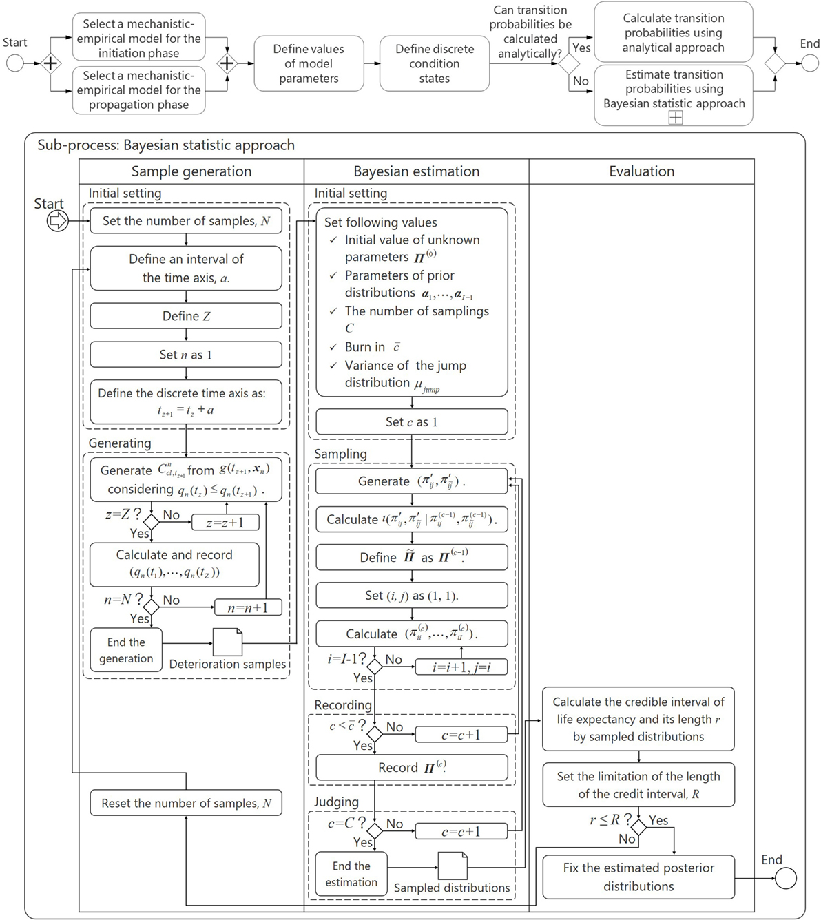
Figure 2. Methodology.

Generate Sample Deterioration Paths

In this step, a set of values for the vector X are generated using its parametric inferences (e.g., mean and SD of a probability distribution). The generated set of values of X is then used, together with the mechanistic-empirical models to generate a sample path of deterioration for the concrete element. N paths are generated, and X_n (n = 1, …, N) denotes X used to generate path n. Path n is considered to be independent from the other paths 1, …, n − 1, n + 1, …, N. These paths are then discretized into Z time intervals as condition states at time points on a discrete time axis t_z+1 = t_z + a (z = 1, …, Z − 1). a is the time interval of the discrete time axis. The condition state of the element associated with path n at time t_z is denoted as q_n(t_z). The sample paths are generated using the following rules:

${\mathrm{\theta }}_{i,j}^{n,z}=\left\{\begin{array}{ll}1\hfill & q_n\left(t_z\right)=i,q_n\left(t_{z+1}\right)=j\hfill \\ 0\hfill & \text{Otherwise}\hfill \end{array}\right.,$ (12)

where ${\mathrm{\theta }}_{i,j}^{n,z}$ is a dummy variable. The total number of sample paths is then expressed as the vector $\mathrm{\Theta }=\left({\mathrm{\theta }}_{1,1}^{1,1},\dots ,{\mathrm{\theta }}_{I,I}^{N,Z}\right)$.

At time t_z+1, the condition value associated with sample path n, is as follows:

$y_{t_{z+1}}^n=g\left(t_{z+1},{\mathit{\text{X}}}_n\right).$ (13)

As the same X_n is used to generate path n, the condition states of the element, for time points t_z and t_z+1, satisfy the following constraint:

$q_n\left(t_z\right)\le q_n\left(t_{z+1}\right)\forall z.$ (14)

Estimate the Transition Probabilities

In this step, Bayesian estimation is used to estimate the transition probabilities. This includes the three sub-steps of

○ specify the initial values of unknown parameters, Π⁽⁰⁾, and the prior probability distribution function p(Π) through the specification of its parameters a₁, …, a_I−1 based on the prior information;

○ define the likelihood function L(Θ, Π) using the obtained data Θ;

○ determine the posterior probability density function p(Π|Θ) as the product of the prior probability density function and the likelihood function in accordance with the Bayes’ theorem.

Here, Π denotes the unknown parameter vector. It is assumed that Π is a random variable and is subjected to the prior probability density function p(Π). Under these conditions and according to Bayes’ theorem (Bayes and Price, 1763), when the observed data Θ are given, the posterior probability density function p(Π|Θ) of the unknown parameters Π is defined as follows:

$p\left(\mathrm{\Pi }|\mathrm{\Theta }\right)=\frac{L\left(\mathrm{\Theta },\mathrm{\Pi }\right)p\left(\mathrm{\Pi }\right)}{{\int }_{\Xi }L\left(\mathrm{\Theta },\mathrm{\Pi }\right)p\left(\mathrm{\Pi }\right)d\mathrm{\Pi }},$ (15)

where Ξ represents the parameter space. At this time, p(Π|Θ) can be expressed as follows:

$p\left(\mathrm{\Pi }|\mathrm{\Theta }\right)\propto L\left(\mathrm{\Theta },\mathrm{\Pi }\right)p\left(\mathrm{\Pi }\right),$ (16)

where the symbol “ ∝” denotes “be proportional to.”

Specify the Prior Probability Distribution

The specification of the prior probability density function requires that the random variables of the prior probability density function have same domains as the unknown parameters. The distribution to be used has to satisfy the condition of the transition probabilities, that is

${\displaystyle \sum _{j=1}^I}{\mathrm{\pi }}_{\mathit{ij}}=1,$ (17)

$0\le {\mathrm{\pi }}_{\mathit{ij}}\le 1.$ (18)

The Dirichlet distribution is a good example. The function of the distribution is given by the following equation:

$p\left({\mathrm{\pi }}_i\right)=\frac{1}{B\left({\mathrm{\pi }}_i\right)}{\displaystyle \prod _{j=1}^I}{\left({\mathrm{\pi }}_{\mathit{ij}}\right)}^{{\mathrm{\alpha }}_{i,j}-1},$ (19)

where B(⋅) is a beta function; π_i = (π_i,1, …, π_i,I) holds; and α_i = (α_i,1, …, α_i,I) is a parameter vector of the Dirichlet distribution.

Define the Likelihood Function

The definition of the likelihood function requires determining the number of sample paths and number of condition states to be used. In the likelihood function, the transition probabilities from condition states i to j are the model parameters and the data used to estimate the transition probabilities are the sample paths generated using the mechanistic-empirical models. The likelihood function, therefore, consists of the probabilities of having specific values of the transition probabilities, as follows:

$L\left(\mathrm{\Theta },\mathrm{\Pi }\right)={\displaystyle \prod _{n=1}^N}{\displaystyle \prod _{z=1}^{Z-1}}{\displaystyle \prod _{i=1}^I}{\displaystyle \prod _{j=i}^I}{\left({\mathrm{\pi }}_{\mathit{ij}}\right)}^{{\mathrm{\theta }}_{i,j}^{n,z}}.$ (20)

Determine the Posterior Probability Density Function

The posterior probability density function p(Π|Θ) is determined through the definition of the unknown parameters. It has the following form:

$p\left(\mathrm{\Pi }|\mathrm{\Theta }\right)=L\left(\mathrm{\Theta },\mathrm{\Pi }\right){\displaystyle \prod _{i=1}^{I-1}}p\left({\mathrm{\pi }}_i\right).$ (21)

The unknown parameters are determined Π^(c) using MCMC simulation with Gibbs sampling (Geman and Geman, 1984) and the random walk Metropolis Hastings (MH) algorithm (Hastings, 1970), and recorded Π^(c). MCMC simulation has been used successfully in this way to estimate the posterior distributions in the past in situations where the multidimensional integration of the objective function of a model was not possible (Robert, 1996).

For each MCMC simulation, the random walk MH algorithm estimates the transition probabilities $\left({\mathrm{\pi }}_{\mathit{ij}}^{\left(c\right)},{\mathrm{\pi }}_{i\tilde{j}}^{\left(c\right)}\right)$ in each loop c(c = 1, …, C) by comparing a candidate set of transition probabilities $\left({\mathrm{\pi }\prime }_{\mathit{ij}},{\mathrm{\pi }\prime }_{i\tilde{j}}\right)$ with a sample $\left({\tilde{\mathrm{\pi }}}_{\mathit{ij}},{\tilde{\mathrm{\pi }}}_{i\tilde{j}}\right)$. ${\tilde{\mathrm{\pi }}}_{\mathit{ij}}$ is the transition probability that is compared with the candidate of transition probabilities. ${\tilde{\mathrm{\pi }}}_{\mathit{ij}}$ is defined as ${\mathrm{\pi }}_{\mathit{ij}}^{\left(c-1\right)}$ and is i × j element of $\tilde{\mathrm{\Pi }}$. The candidate set of transition probabilities must satisfy the constraint of the Markov model, ${\sum }_{j=i}^I{\mathrm{\pi }}_{\mathit{ij}}=1$. Here, $\tilde{j}$ represents the state that is most likely to occur. For example, when i = 1, I = 4, and j = 2, and the transition probabilities are (π_i1, …, π_i4) = (0.1, 0.1, 0.7, 0.1), $\tilde{j}$ becomes 3. When ${\mathrm{\pi }\prime }_{\mathit{ij}}$ is generated so that the sum of ${\mathrm{\pi }\prime }_{\mathit{ij}}$ and ${\mathrm{\pi }\prime }_{i\tilde{j}}$ is same as the sum of ${\tilde{\mathrm{\pi }}}_{\mathit{ij}}$ and ${\tilde{\mathrm{\pi }}}_{i\tilde{j}}$, ${\sum }_{j=i}^I{\mathrm{\pi }}_{\mathit{ij}}=1$ is satisfied. At this time, ${\mathrm{\pi }\prime }_{\mathit{ij}}$ has to be within the interval [0, U], and $U={\tilde{\mathrm{\pi }}}_{\mathit{ij}}+{\tilde{\mathrm{\pi }}}_{i\tilde{j}}$ holds. To do this, ${\mathrm{\pi }\prime }_{\mathit{ij}}$ is generated using a truncated normal distribution with mean ${\tilde{\mathrm{\pi }}}_{\mathit{ij}}$, on [0, U] and variance μ_jump, $\mathrm{\psi }\left({\mathrm{\pi }\prime }_{\mathit{ij}},{\tilde{\mathrm{\pi }}}_{\mathit{ij}},{\mathrm{\mu }}_{\text{jump}},U\right)$. When ${\mathrm{\pi }\prime }_{\mathit{ij}}$ is generated, ${\mathrm{\pi }\prime }_{i\tilde{j}}$ is fixed uniquely as ${\mathrm{\pi }\prime }_{i\tilde{j}}=U-{\mathrm{\pi }\prime }_{\mathit{ij}}$. Thus, the occurrence probability of ${\mathrm{\pi }\prime }_{\mathit{ij}}$ corresponds to the joint occurrence probability of the set $\left({\mathrm{\pi }\prime }_{\mathit{ij}},{\mathrm{\pi }\prime }_{i\tilde{j}}\right)$, $\mathrm{\zeta }\left({\mathrm{\pi }\prime }_{\mathit{ij}},{\mathrm{\pi }\prime }_{i\tilde{j}}|{\tilde{\mathrm{\pi }}}_{\mathit{ij}},{\tilde{\mathrm{\pi }}}_{i\tilde{j}}\right)$, as follows:

$\mathrm{\psi }\left({\mathrm{\pi }\prime }_{\mathit{ij}},{\tilde{\mathrm{\pi }}}_{\mathit{ij}},{\mathrm{\mu }}_{\text{jump}},U\right)=\mathrm{\zeta }\left({\mathrm{\pi }\prime }_{\mathit{ij}},{\mathrm{\pi }\prime }_{i\tilde{j}}|{\tilde{\mathrm{\pi }}}_{\mathit{ij}},{\tilde{\mathrm{\pi }}}_{i\tilde{j}}\right)=\frac{\frac{1}{{\mathrm{\mu }}_{\text{jump}}}\mathrm{\varphi }\left(\frac{{\mathrm{\pi }\prime }_{\mathit{ij}}-{\tilde{\mathrm{\pi }}}_{\mathit{ij}}}{{\mathrm{\mu }}_{\text{jump}}}\right)}{\mathrm{\Phi }\left(\frac{U-{\tilde{\mathrm{\pi }}}_{\mathit{ij}}}{{\mathrm{\mu }}_{\text{jump}}}\right)-\mathrm{\Phi }\left(\frac{0-{\tilde{\mathrm{\pi }}}_{\mathit{ij}}}{{\mathrm{\mu }}_{\text{jump}}}\right)},$ (22)

where ${\tilde{\mathrm{\pi }}}_{\mathit{ij}}$ is the expected value, μ_jump is the variance, and ${\mathrm{\pi }\prime }_{i\tilde{j}}$ is $U-{\mathrm{\pi }\prime }_{\mathit{ij}}$. ϕ(⋅) is a probability density function of a standard normal distribution, and Φ(⋅) is a cumulative distribution function of a standard normal distribution. The probability that a candidate set $\left({\mathrm{\pi }\prime }_{\mathit{ij}},{\mathrm{\pi }\prime }_{i\tilde{j}}\right)$ is accepted is expressed as follows:

$\mathrm{\iota }\left({\mathrm{\pi }\prime }_{\mathit{ij}},{\mathrm{\pi }\prime }_{i\tilde{j}}|{\tilde{\mathrm{\pi }}}_{\mathit{ij}},{\tilde{\mathrm{\pi }}}_{i\tilde{j}}\right)=\min \left(\frac{p\left(\mathrm{\Theta },{\tilde{\mathrm{\Pi }}}_{-\left(i,j\right)\left(i,\tilde{j}\right)},{\mathrm{\pi }\prime }_{\mathit{ij}},{\mathrm{\pi }\prime }_{i\tilde{j}}\right)\mathrm{\zeta }\left({\mathrm{\pi }\prime }_{\mathit{ij}},{\mathrm{\pi }\prime }_{i\tilde{j}}|{\tilde{\mathrm{\pi }}}_{\mathit{ij}},{\tilde{\mathrm{\pi }}}_{i\tilde{j}}\right)}{p\left(\mathrm{\Theta },{\tilde{\mathrm{\Pi }}}_{-\left(i,j\right)\left(i,\tilde{j}\right)},{\tilde{\mathrm{\pi }}}_{\mathit{ij}},{\tilde{\mathrm{\pi }}}_{i\tilde{j}}\right)\mathrm{\zeta }\left({\tilde{\mathrm{\pi }}}_{\mathit{ij}},{\tilde{\mathrm{\pi }}}_{i\tilde{j}}|{\mathrm{\pi }\prime }_{\mathit{ij}},{\mathrm{\pi }\prime }_{i\tilde{j}}\right)},1\right),$ (23)

where ${\tilde{\mathrm{\Pi }}}_{-\left(i,j\right)\left(i,\tilde{j}\right)}$ is the parameter set which consists of $\tilde{\mathrm{\Pi }}$ except ${\tilde{\mathrm{\pi }}}_{\mathit{ij}}$ and ${\tilde{\mathrm{\pi }}}_{i\tilde{j}}$. Equation 23 means that a candidate is accepted with probability 1 if it has a better fit with the paths, and a candidate is accepted with the probability formulated as a ratio of the product of the posterior probability density function and the occurrence probability of the candidate if it does not have a better fit with paths. Using this probability, parameters following the posterior distribution are sampled numerically avoiding falling into local optima.

$\left({\tilde{\mathrm{\pi }}}_{\mathit{ij}},{\tilde{\mathrm{\pi }}}_{i\tilde{j}}\right)$ is sampled as follows:

$\left({\tilde{\mathrm{\pi }}}_{\mathit{ij}},{\tilde{\mathrm{\pi }}}_{i\tilde{j}}\right)=\left\{\begin{array}{ll}\left({\tilde{\mathrm{\pi }}}_{\mathit{ij}},{\tilde{\mathrm{\pi }}}_{i\tilde{j}}\right)\hfill & u_c^i>\mathrm{\iota }\left({\mathrm{\pi }\prime }_{\mathit{ij}},{\mathrm{\pi }\prime }_{i\tilde{j}}|{\tilde{\mathrm{\pi }}}_{\mathit{ij}},{\tilde{\mathrm{\pi }}}_{i\tilde{j}}\right)\hfill \\ \left({\mathrm{\pi }\prime }_{\mathit{ij}},{\mathrm{\pi }\prime }_{i\tilde{j}}\right)\hfill & u_c^i\le \mathrm{\iota }\left({\mathrm{\pi }\prime }_{\mathit{ij}},{\mathrm{\pi }\prime }_{i\tilde{j}}|{\tilde{\mathrm{\pi }}}_{\mathit{ij}},{\tilde{\mathrm{\pi }}}_{i\tilde{j}}\right)\hfill \end{array}\right.,$ (24)

where $u_c^i$ is a uniform random number drawn from the uniform distribution whose domain is [0,1]. In Gibbs sampling, $\left({\tilde{\mathrm{\pi }}}_{\mathit{ij}},{\tilde{\mathrm{\pi }}}_{i\tilde{j}}\right)$ can be sampled from the other elements of $\tilde{\mathrm{\Pi }}$. In the iterative procedure, the elements of $\tilde{\mathrm{\Pi }}$ are defined successively in order from j = i to j = I in each i, and $\left({\mathrm{\pi }}_{\mathit{ii}}^{\left(c\right)},\dots ,{\mathrm{\pi }}_{\mathit{iI}}^{\left(c\right)}\right)$ is fixed as $\left({\tilde{\mathrm{\pi }}}_{\mathit{ii}},\dots ,{\tilde{\mathrm{\pi }}}_{\mathit{iI}}\right)$ if j = I.

Evaluate the Results

A Geweke test statistic (Geweke, 1992) is used to evaluate convergence during sampling. The Geweke test statistic indicates difference between the first 10% $\left({\mathrm{\Pi }}^{\left(\overline{c}+1\right)},\dots ,{\mathrm{\Pi }}^{\left(0.1\left(C-\overline{c}\right)+\overline{c}\right)}\right)$ and the last 50% $\left({\mathrm{\Pi }}^{\left(0.5\left(C-\overline{c}\right)+\overline{c}\right)},\dots ,{\mathrm{\Pi }}^{\left(C\right)}\right)$ of sampled transition probabilities. $\overline{c}$ is burn-in. A statistical hypothesis test is conducted using the Geweke test statistic. When the statistics are less than 1.96 (significance level 5%), it is judged that sampling has converged and $\left({\mathrm{\Pi }}^{\left(\overline{c}+1\right)},\dots ,{\mathrm{\Pi }}^{\left(C\right)}\right)$ are samples from the posterior distribution.

The expected transition probabilities, which are used as the estimated values, are then given by the following equation:

${\tilde{\mathrm{\pi }}}_{\mathit{ij}}=\frac{{\sum }_{c=\overline{c}+1}^C{\mathrm{\pi }}_{\mathit{ij}}^{\left(c\right)}}{C-\overline{c}}\left(i=1,\dots ,I-1;j=i,\dots ,I\right).$ (25)

The 100(1 − 2κ)% Bayesian credible interval of each parameter, $\left[{\underset{¯}{\mathrm{\pi }}}_{\mathit{ij}}^{\mathrm{\kappa }},{\overline{\mathrm{\pi }}}_{\mathit{ij}}^{\mathrm{\kappa }}\right]$, is calculated by $\left({\mathrm{\Pi }}^{\left(\overline{c}+1\right)},\dots ,{\mathrm{\Pi }}^{\left(C\right)}\right)$ as follows:

${\underset{¯}{\mathrm{\pi }}}_{\mathit{ij}}^{\mathrm{\kappa }}=\arg \underset{{\mathrm{\pi }}_{\mathit{ij}}^{\ast }}{\max }\left\{\frac{\#\left({\mathrm{\pi }}_{\mathit{ij}}^{\left(c\right)}\le {\mathrm{\pi }}_{\mathit{ij}}^{\ast },c=\overline{c}+1,\mathrm{\dots },C\right)}{C-\overline{c}}\le \mathrm{\kappa }\right\},$ (26)

${\overline{\mathrm{\pi }}}_{\mathit{ij}}^{\mathrm{\kappa }}=\arg \underset{{\mathrm{\pi }}_{\mathit{ij}}^{\ast \ast }}{\max }\left\{\frac{\#\left({\mathrm{\pi }}_{\mathit{ij}}^{\left(c\right)}\ge {\mathrm{\pi }}_{\mathit{ij}}^{\ast \ast },c=\overline{c}+1,\mathrm{\dots },C\right)}{C-\overline{c}}\le \mathrm{\kappa }\right\}.$ (27)

Here, the symbol #(⋅) indicates the number of c that satisfies the logical expression in parentheses. $\left[{\underset{¯}{\mathrm{\pi }}}_{\mathit{ij}}^{\mathrm{\kappa }},{\overline{\mathrm{\pi }}}_{\mathit{ij}}^{\mathrm{\kappa }}\right]$ indicates that the probability that the expected transition probability lies in $\left[{\underset{¯}{\mathrm{\pi }}}_{\mathit{ij}}^{\mathrm{\kappa }},{\overline{\mathrm{\pi }}}_{\mathit{ij}}^{\mathrm{\kappa }}\right]$ is 1 − 2κ.

The length of time required to transition to condition state i − 1 (i = 2, …, I) and i in the deterioration path of s%, $l_{i,s}^{\left(c\right)}$, is calculated using following equation:

$l_{i,s}^{\left(c\right)}=t_{\tilde{z}}+\frac{a\left(\frac{s}{100}-{\sum }_{j=1}^i{\mathrm{\nu }}_{j,t_{\tilde{z}}}^{\left(c\right)}\right)}{{\sum }_{j=1}^i{\mathrm{\nu }}_{j,t_{\tilde{z}}+1}^{\left(c\right)}-{\sum }_{j=1}^i{\mathrm{\nu }}_{j,t_{\tilde{z}}}^{\left(c\right)}}-l_{i-1,s}^{\left(c\right)},$ (28)

where

$\tilde{z}=\max z\text{Subject}\text{to}{\displaystyle \sum _{j=1}^i}{\mathrm{\nu }}_{j,t_z}^{\left(c\right)}\le \frac{s}{100},$ (29)

where $l_{1,s}^{\left(c\right)}=0$ and ${\mathrm{\nu }}_{j,t_z}^{\left(c\right)}$ is jth element of state vector ${\mathrm{\nu }}^{\left(c\right)}\left(t_z\right)$ at t_z calculated by ${\mathrm{\Pi }}^{\left(c\right)}$. $l_{i,s}^{\left(c\right)}$ is defined so that the probability that length of time required to transition to condition state i − 1 (i = 2, …, I) and i is less than $l_{i,s}^{\left(c\right)}$ is s%. The first term on the right hand side of Eq. 28 is the expected length of time to transition from the initial time point to condition state i. The second is the condition value obtained from the mechanistic-empirical model. The ratio of the difference between ${\sum }_{j=1}^i{\mathrm{\nu }}_{j,t_{\tilde{z}}}^{\left(c\right)}$ and s/100 is added to the difference between ${\sum }_{j=1}^i{\mathrm{\nu }}_{j,t_{\tilde{z}}}^{\left(c\right)}$ and ${\sum }_{j=1}^i{\mathrm{\nu }}_{j,t_{\tilde{z}}+1}^{\left(c\right)}$ to express the length of time more precisely. For example, when a = 1, ${\sum }_{j=1}^i{\mathrm{\nu }}_{j,t_{\tilde{z}}+1}^{\left(c\right)}=0.33$, ${\sum }_{j=1}^i{\mathrm{\nu }}_{j,t_{\tilde{z}}+1}^{\left(c\right)}=0.27$, and s = 30(%), 1 × (30/100 − 0.27)/(0.33 − 0.27) = 0.5 is added to $t_{\tilde{z}}$ to evaluate the length of time between $t_{\tilde{z}}$ and $t_{\tilde{z}+1}$. For example, when $t_{\tilde{z}}=20$ and $t_{\tilde{z}+1}=t_{\tilde{z}}+a=21$, the sum of the first and second term on the right hand side of Eq. 28 is calculated as 20.5.

The estimated transition probabilities are evaluated using the Bayesian credible intervals of expected length of time required to transition between condition states. The Bayesian credible interval of the expected length of time to make transitions between condition states 1 and I is $T^{\left(c\right)}={\sum }_{i=1}^I{l}_{i,50}^{\left(c\right)}$. The 100(1 − 2κ)% Bayesian credible interval of the expected duration $T^{\left(c\right)}\left(c=\overline{c},\dots ,C\right)$ is defined as $\left[{\underset{¯}{T}}^{\mathrm{\kappa }},{\overline{T}}^{\mathrm{\kappa }}\right]$, i.e., the probability that the expected duration lies in $\left[{\underset{¯}{T}}^{\mathrm{\kappa }},{\overline{T}}^{\mathrm{\kappa }}\right]$ is 1 − 2κ, treating the expected length of time as a random variable. The magnitude of the difference $r={\overline{T}}^{\mathrm{\kappa }}-{\underset{¯}{T}}^{\mathrm{\kappa }}$ can be used to determine how good the estimated values are. If they are good enough, then the estimated transition probabilities are considered correct. If not, then more sample paths are generated using the mechanistic-empirical models and the process is started over again. This process is illustrated in the sub-process of Figure 2.

${\underset{¯}{T}}^{\mathrm{\kappa }}$ and ${\overline{T}}^{\mathrm{\kappa }}$ are defined as sample order statistics as follows:

${\underset{¯}{T}}^{\mathrm{\kappa }}=\arg \underset{T^{\ast }}{\max }\left\{\frac{\#\left(T^{\left(c\right)}\le T^{\ast },c=\overline{c}+1,\mathrm{\dots },C\right)}{C-\overline{c}}\le \mathrm{\kappa }\right\},$ (30)

${\overline{T}}^{\mathrm{\kappa }}=\arg \underset{T^{\ast \ast }}{\max }\left\{\frac{\#\left(T^{\left(c\right)}\ge T^{\ast \ast },c=\overline{c}+1,\mathrm{\dots },C\right)}{C-\overline{c}}\le \mathrm{\kappa }\right\}.$ (31)

Here, the symbol #(⋅) indicates the number of c which satisfies the logical expression in parentheses. As shown in Figure 2, using a threshold value R that is established in advance and depends on the desired amount of accuracy. If r is smaller than R, the algorithm is controlled to be stopped. On the other hand, if r is greater than R, the algorithm returns to the sample generation phase and redefine N.

Example

Overview

The methodology was tested by using it to estimate the transition probabilities for a reinforced concrete element. The mechanistic-empirical models used for the initiation phase and the propagation phase were given by the following equations:

$y_1=g_1\left(t_z,x_{1,1}\right)=C_s\left(1-\text{erf}\left[\frac{d}{2\sqrt{x_{1,1}{t}_z}}\right]\right)$ (32)

and

$y_2=g_2\left(t_z,x_{2,1},x_{2,2}\right)=x_{2,1}+{\left(t_z\right)}^2\frac{x_{2,2}}{2},$ (33)

respectively.

In these equations, x_1,1, x_2,1, and x_2,2 were considered as random variables. As information about distributions of the parameters C_s, x_cl, D_cl, V_corr, α, wet, w₀, β, and P₀ in Eqs 2–4 was not available, they are summarized as C_s = C_s, d = x_cl, x_1,1 = D_cl, x_2,1 = w₀ − βP₀, and x_2,2 = β*V_corr*α*wet in Eqs 32 and 33, and it is assumed that x_1,1, x_2,1, and x_2,2 are distributed based on normal distributions. The values of these variables used are shown in Table 1.

TABLE 1

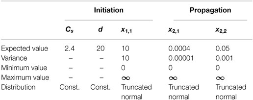
Table 1. Parameters of ME model.

The condition values obtained from Eqs 32 and 33 were mapped to condition state as shown in Table 2.

TABLE 2

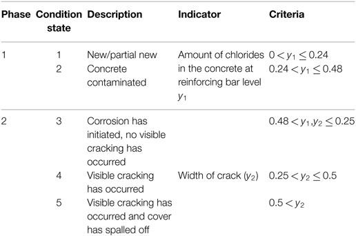
Table 2. Definition of condition states.

Estimation Based on Relationship between Mechanistic-Empirical Models and Transition Probabilities

When the mechanistic-empirical models in Eqs 32 and 33 are used, the transition probabilities cannot be estimated analytically based on their relationship shown in Section “Relationship between Mechanistic-Empirical Models and Transition Probabilities.” The transition probabilities π₁₁ and π₁₂, however, can be estimated with numerical integration (e.g., Monte Carlo simulation) based on the relationship between the initiation model and the transition probabilities because the initiation model includes a single random variable x_1,1. Here, as an example, π₁₁(1) is estimated. It can be expressed, using probability density functions of a truncated normal distribution and a continuous uniform distribution, as follows:

$\mathrm{\pi }\left(1\right)=\frac{1}{t_Z}{\int }_0^{t_Z}H\left(m\left(y_i,t\right);10,\sqrt{10},0,\infty \right)-H\left(m\left(y_{i-1},t\right);10,\sqrt{10},0,\infty \right)\mathit{dt},$ (34)

where H(⋅; h_mean, h_sd, h_l, h_u) is the cumulative distribution function of the truncated normal distribution with mean h_mean, SD h_sd, and support [h_l, h_u]. In addition, π(1, 1, 1) can be formulated as follows:

$\mathrm{\pi }\left(1,1,1\right)=\frac{1}{t_Z}{\int }_0^{t_Z}H\left(m\left(\underset{¯}{y},t\right);10,\sqrt{10},0,\infty \right)-H\left(m\left(\underset{¯}{y},t\right);10,\sqrt{10},0,\infty \right)\mathit{dt},$ (35)

and, therefore

${\mathrm{\pi }}_{11}\left(1\right)=\frac{\mathrm{\pi }\left(1,1,1\right)}{\mathrm{\pi }\left(1\right)}.$ (36)

As π(1, 1, 1) = 0.0754 and π(1) = 0.0858 by computation using Monte Carlo simulation to solve integration in Eqs 35 and 36, π₁₁(1) is 0.879. Estimation of the transition probabilities with the proposed Bayesian approach can be regarded as solving the integrations by generating sample deterioration paths and statistically estimating the transition probabilities instead of using numerical integration. As estimated result can be evaluated using posterior distributions and Bayesian credible intervals, the proposed Bayesian approach is superior to the numerical integration when the integration cannot be solved analytically.

Generate Sample Deterioration Paths

To estimate the other transition probabilities, a set of sample paths (N = 10,000) was generated for 1-year time intervals over a period of 100 years, i.e., a = 1, Z = 100.

Estimate Transition Probabilities

The estimated transition probabilities are shown in Table 3. Comparing π₁₁(1) between the Bayesian approach and the approach based on relationship between mechanistic-empirical models and transition probabilities, it can be found that π₁₁(1) = 0.879 derived in 7.2 fits well to the result with the proposed Bayesian approach.

TABLE 3

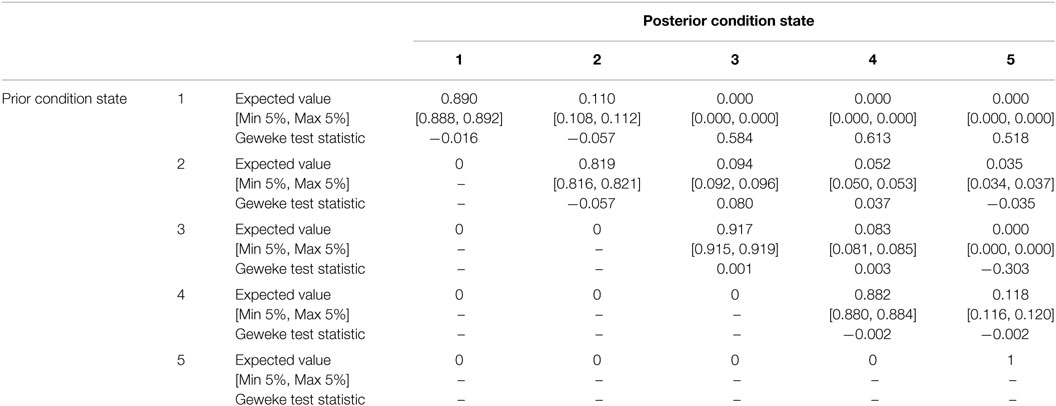
Table 3. Estimated Markov transition probabilities.

Evaluate Results

To calculate Bayesian credible intervals of the expected length of the transition between condition states, the transition probabilities obtained in every step of the MCMC simulation were used. C and $\overline{c}$ were set to 11,000 and 1,000, respectively. In sampling $c\left(c=\overline{c},\dots ,C\right)$, the expected duration $l_{i,s}^{\left(c\right)}$ was calculated from the transition probability matrix Π^(c) and Eq. 28.

The suitability of the number of generated paths N were evaluated using

○ a distribution of the length of time to transition from condition state 1–5 with s = 50 (%), T^(c),

○ a 90% Bayesian credible interval, $\left[{\underset{¯}{T}}^5,{\overline{T}}^5\right]$ (with $\left[{\underset{¯}{T}}^5,{\overline{T}}^5\right]=\left[23.704\left(\text{years}\right),24.229\left(\text{years}\right)\right]$, $r={\overline{T}}^5-{\underset{¯}{T}}^5=0.525\left(\text{years}\right)$), and

○ R = 1 (year).

The Bayesian credible intervals and Geweke test statistics are shown in Table 3. As r ≤ R and all of the Geweke test statistics are less than 1.96 (significance level 5%), it is concluded that 10,000 deterioration paths were sufficient to estimate the transition probabilities.

Discussion

By using the estimated values of the Markov transition probabilities, deterioration processes can be expressed stochastically as transition of the condition state vector over time. Figure 3A shows the transition of values of the condition vector calculated based on the transition probabilities estimated with the proposed methodology. The results shown in Figure 3A enable the evaluation of the condition at arbitrary time points, as well as the deterioration paths. Considering the state vectors estimated using the Markov model, probability s that the reinforced concrete element in each condition state can be used as a risk control level. Figure 4 shows deterioration paths with different risk control levels. These can be used to determine the points in time when inspections should be performed or interventions should be executed.

FIGURE 3

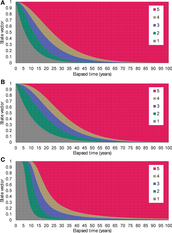
Figure 3. Transition of state vector over time: (A) calculated using the transition probabilities estimated by the proposed methodology; (B) calculated using the transition probabilities estimated by the state-of-the-art methodology; and (C) calculated using the mechanistic-empirical models.

FIGURE 4

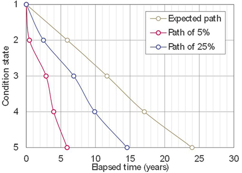
Figure 4. Deterioration paths.

Comparison with the State-of-the-Art

The comparison between the proposed methodology and the state-of-the-art methodology (Lethanh et al., 2017) was done by estimating the transition probabilities using both methodologies from the mechanistic-empirical models shown in Eqs 32 and 33 and Table 1, and measuring the differences (or residuals) between the average condition values predicted by using the Markov models and the condition values predicted using the mechanistic-empirical models. Figure 3B shows the state vectors calculated using transition probabilities estimated by the state-of-the-art methodology shown in Table 4. The condition state distributions for each time interval calculated by the mechanistic-empirical models are shown in Figure 3C, i.e., the condition state distributions in Figure 3C are calculated as ratios of condition states at each time point in the generated sample deterioration paths in 7.3. The values of the log likelihood with the transition probabilities estimated using the proposed methodology and the state-of-the-art methodology were −1.0924E+05 and −1.2697E+05, respectively. The proposed methodology can maximize the likelihood function and fit transition probabilities to generated sample paths better than the state-of-the-art methodology. To discuss the results in detail, the differences of sums of squared residuals between the Markov models and the condition values predicted using the mechanistic-empirical models are given in Table 5. This table shows, for example, that the sum of squared residuals in the period between 11 and 20 years was 4.20E−01. It can be seen that the differences between 11 and 60 years using the models developed with the proposed methodology are smaller than the differences using the models developed with the state-of-the-art methodology. This tendency can be seen in the expected deterioration paths shown in Figure 5 as the path of the proposed methodology is closer to that of data than the state-of-the-art methodology after 10 years elapsed.

TABLE 4

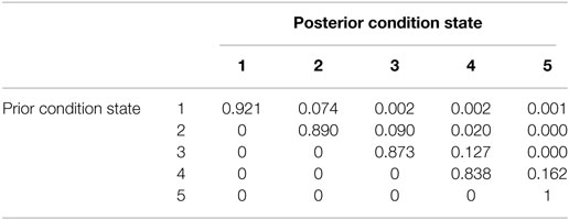
Table 4. Estimated transition probabilities using state-of-the-art methodology.

TABLE 5

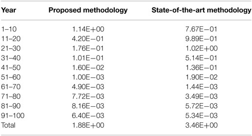
Table 5. Sum of the differences between the condition values predicted using the Markov models and those predicted using the mechanistic-empirical models.

FIGURE 5

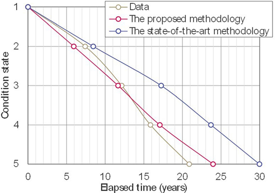
Figure 5. Comparison among expected deterioration paths.

From Table 5, it can be also seen that the sums of differences over 100 years were 1.88 condition states and 3.46 condition states using the Markov models developed using the proposed and the state-of-the-art methodologies, respectively. From these results, it can be inferred that the Markov model developed using the state-of-the-art methodology overestimates life expectancy and underestimates the speed of deterioration because the result of the state-of-the-art methodology was influenced excessively by the data between 61 and 100 years to estimate transition probabilities π_3j, π_4j, and π_5j.

The Number of Deterioration Paths from the Mechanistic-Empirical Models

In the proposed methodology, the accuracy of the Markov models depends on the number of deterioration paths N used in the estimation of the transition probabilities. This relationship is shown in Figure 6 and Table 6 for all transition probabilities for values of N ranging between 1,000 and 10,000 at 1,000 step intervals. In all cases, as above, the following values were used a = 1 (year), $\overline{c}=1,000$, and Z = 100. The posterior distributions calculated using sampled parameter π₁₁(1) are shown in Figure 7 for N = 1,000 and N = 10,000 as an example. From Figures 6 and 7 and Table 6, it can be seen that the parameter dispersion decreases from 1.16E−02 to 3.39E−03 as N increases from 1,000 to 10,000. As shown in Table 6, all of the other parameters π_ij have the same magnitude correlation to the case of π₁₁ as N increases from 1,000 to 10,000. The credible interval of π₁₅ with N = 4,000 is not shown in Table 6 because all sampled π₁₅ were 0.

FIGURE 6

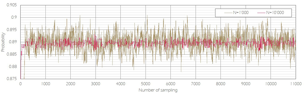
Figure 6. Sampling of parameter π11(1).

TABLE 6

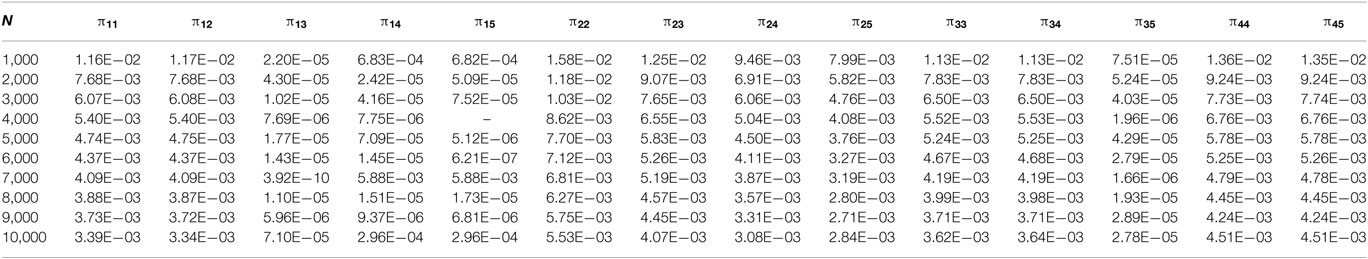
Table 6. 90% Bayesian credible intervals of transition probabilities.

FIGURE 7

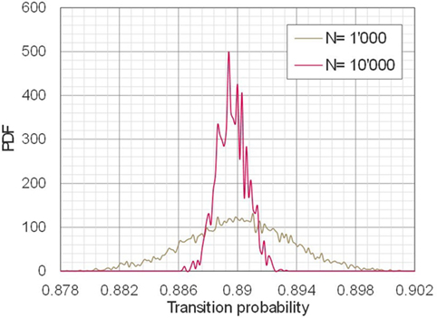
Figure 7. Posterior distributions of π11(1).

It can be seen in the previous table and in Figure 8, which shows the 90% Bayesian credible intervals of life expectancies with N from 1,000 to 10,000 at 1,000 step intervals that the Bayesian credible intervals vary as a function of the number of deterioration paths used. With a threshold of R = 1 (year), where $r={\overline{T}}^5-{\underset{¯}{T}}^5$, it seen that N is to be at least 3,000 to obtain a satisfactory result. Figure 9 indicates that the required N increases when R decreases. From Figure 9, it can be seen that N has to be greater than 5,000 or more when R = 0.8 (years), and 8,000 or more when R = 0.6 (years), respectively.

FIGURE 8

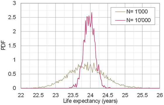
Figure 8. Distributions of life expectancies.

FIGURE 9

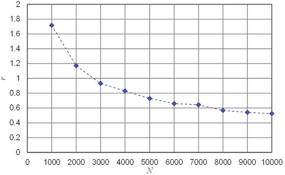
Figure 9. 90% Bayesian credible intervals of life expectancies.

Conclusion

In this article, a methodology is presented to estimate the transition probabilities to be used in Markov models from mechanistic-empirical models. The methodology can be used when there is little to no available time-series inspection information, but mechanistic-empirical models are available. The proposed methodology includes the use of analytical solutions where possible and the use of Bayesian statistics where analytical solutions are not possible. When the Bayesian approach is used, the accuracy of the transition probabilities is to be estimated as a function of the number of deterioration paths calculated.

The methodology is demonstrated by using it to estimate the transition probabilities to be used in a Markov model for reinforced concrete bridge elements deteriorating due to chloride-induced corrosion of the reinforcement. It was shown in this example that the proposed methodology was an improvement on the state-of-the-art methodology, as the sum of residuals over 100 years with the proposed methodology was 100*1.88/3.46 = 54% of that of the state-of-the-art methodology, i.e., the proposed methodology gave a 46% point decrease. In addition, the later would have over-estimated the speed of deterioration.

In the work presented in this article, it was assumed that stationary transition probabilities are to be used. When Markov models with stationary transition probabilities are used, certain limitations are imposed which restrict the modeling of the deterioration processes. This is considered to be okay if the sum of residuals is close to 0. If, however, it is found that they do not, the use of non-stationary transition probabilities might provide better results. The use of non-stationary transition probabilities could improve the modeling of deterioration in these circumstances. They could, for example, be used to capture sudden decreases in the states elements. Future work should be focused on the use of non-stationary transition probabilities in bridge management systems. Some preliminary work is that done by Wellalage (2015).

In addition, the proposed methodology has potential of use for many other materials in addition to reinforced concrete, in situations where condition data are not available but mechanistic-empirical models are available. Exactly how this should be done is, for each type of material, a topic for future work.

Author Contributions

DM contributed to theoretical formulation, program coding, computation, and preparation of the manuscript. BA, NL, and KK contributed to preparation of the manuscript.

Conflict of Interest Statement

NL is employed by POMPLUS Consulting Ltd. All other authors declare no competing interests.

References

AASHTO. (2004). Pontis Release 4.0 Technical Manual. Washington, DC: AASHTO.

Google Scholar

Bayes, T., and Price, R. (1763). An essay towards solving a problem in the doctrine of chances. By the Late Rev. Mr. Bayes, F. R. S. Communicated by Mr. Price, in a Letter to John Canton, A. M. F. R. S. Philos. Trans. R. Soc. Lond. 53, 370–418. doi: 10.1098/rstl.1763.0044

CrossRef Full Text | Google Scholar

Carnahan, J. V., Davis, W. J., Shahin, M. Y., Keane, P. L., and Wu, M. I. (1987). Optimal maintenance decisions for pavement management. J. Transp. Eng. 113, 554–572. doi:10.1061/(ASCE)0733-947X(1987)113:5(554)

CrossRef Full Text | Google Scholar

DuraCrete. (1998). Modelling of Degradation: Duracrete, Probabilistic Performance Based Durability Design of Concrete Structures. Luxembourg: European Union.

Google Scholar

DuraCrete. (2000). Statistical Quanti Cation of the Variables in the Limit State Functions. Luxembourg: European Union.

Google Scholar

Fick, A. (1855). Ueber diffusion. Ann. Phys. 170, 59–86. doi:10.1002/andp.18551700105

CrossRef Full Text | Google Scholar

Geman, S., and Geman, D. (1984). Stochastic relaxation, Gibbs distributions, and the Bayesian restoration of images. IEEE Trans. Pattern Anal. Mach. Intell. 6, 721–741. doi:10.1109/TPAMI.1984.4767596

PubMed Abstract | CrossRef Full Text | Google Scholar

Gertsbakh, I. (2000). Reliability Theory with Applications to Preventive Maintenance. Berlin: Springer.

Google Scholar

Geweke, J. (1992). Evaluating the accuracy of sampling-based approaches to the calculation of posterior moments. Bayesian Stat. 4, 169–193.

Google Scholar

Golroo, A., and Tighe, S. L. (2012). Development of pervious concrete pavement performance models using expert opinions. J. Transp. Eng. 138, 634–648. doi:10.1061/(ASCE)TE.1943-5436.0000363

CrossRef Full Text | Google Scholar

Hastings, W. K. (1970). Monte Carlo sampling methods using Markov chains and their applications. Biometrika 57, 97–109. doi:10.1093/biomet/57.1.97

CrossRef Full Text | Google Scholar

Howard, R. A. (1960). Dynamic Programming and Markov Processes. Massachusetts: The MIT Press.

Google Scholar

Indiana Department of Transportation. (2013). Pavement and Underdrain Design Elements. Indiana Department of Transportation

Google Scholar

Jiang, Y., Saito, M., and Sinha, K. C. (1988). Bridge performance prediction model using the Markov chain. Transp. Res. Rec. 1180, 25–32.

Google Scholar

Kirkpatricka, T. J., Weyers, R. E., Anderson-Cook, C. M., and Sprinkel, M. M. (2002). Probabilistic model for the chloride-induced corrosion service life of bridge decks. Cem. Concr. Res. 32, 1943–1960. doi:10.1016/S0008-8846(02)00905-5

CrossRef Full Text | Google Scholar

Klein, M. (1962). Inspection-maintenance-replacement schedules under Markovian deterioration. Manage. Sci. 9, 25–32. doi:10.1287/mnsc.9.1.25

CrossRef Full Text | Google Scholar

Kobayashi, K., Kaito, K., and Lethanh, N. (2012a). A Bayesian estimation method to improve deterioration prediction for infrastructure system with Markov chain model. Int. J. Archit. Eng. Constr. 1, 1–13. doi:10.7492/IJAEC.2012.001

CrossRef Full Text | Google Scholar

Kobayashi, K., Kaito, K., and Lethanh, N. (2012b). A statistical deterioration forecasting method using hidden Markov model for infrastructure management. Transp. Res. B Methodol. 46, 544–561. doi:10.1016/j.trb.2011.11.008

CrossRef Full Text | Google Scholar

Kolowrocki, K. (2014). Reliability of Large and Complex Systems. Amsterdam: Elsevier Ltd.

Google Scholar

Lancaster, T. (1990). The Econometric Analysis of Transition Data. Cambridge: Cambridge University Press.

Google Scholar

Lee, T. C. (1970). Estimating the Parameters of the Markov Probability Model from Aggregate Time Series Data. Amsterdam: North-Holland Pub. Co.

Google Scholar

Lethanh, N., Hackl, J., and Adey, B. T. (2017). Determination of Markov transition probabilities to be used in bridge management from mechanistic-empirical models. J. Bridge Eng. 22, 4017063. doi:10.1061/(ASCE)BE.1943-5592.0001101

CrossRef Full Text | Google Scholar

Lethanh, N., Kaito, K., and Kobayashi, K. (2015). Infrastructure deterioration prediction with a Poisson hidden Markov model on time series data. J. Infrastruct. Syst. 21, 1–10. doi:10.1061/(ASCE)IS.1943-555X.0000242

CrossRef Full Text | Google Scholar

Madanat, S., and Ben-Akiva, M. (1994). Optimal inspection and repair policies for infrastructure facilities. Transp. Sci. 28, 55–62. doi:10.1287/trsc.28.1.55

CrossRef Full Text | Google Scholar

Mishalani, R. G., and Madanat, S. M. (2002). Computation of infrastructure transition probabilities using stochastic duration models. J. Infrastruct. Syst. 8, 139–148. doi:10.1061/(ASCE)1076-0342(2002)8:4(139)

CrossRef Full Text | Google Scholar

Mizutani, D., Matsuoka, K., and Kaito, K. (2013). Statistical deterioration prediction model considering the heterogeneity in deterioration rates by hierarchical Bayesian estimation. Struct. Eng. Int. 23, 394–401. doi:10.2749/101686613X13627351081515

CrossRef Full Text | Google Scholar

Puterman, M. L. (1994). Markov Decision Process. New Jersey: Wiley.

Google Scholar

Robelin, C.-A., and Madanat, S. M. (2007). History-dependent bridge deck maintenance and replacement optimization with Markov decision processes. J. Infrastruct. Syst. 13, 195–201. doi:10.1061/(ASCE)1076-0342(2007)13:3(195)

CrossRef Full Text | Google Scholar

Robert, C. P. (1996). “Mixtures of distributions: inference and estimation,” in Markov Chain Monte Carlo in Practice, eds W. R. Gillks, S. Richardson, and D. J. Spiegelhalter (London: Chapman and Hall), 442–464.

Google Scholar

Roelfstra, G., Hajdin, R., Adey, B. T., and Brühwiler, E. (2004). Condition evolution in bridge management systems and corrosion-induced deterioration. J. Bridge Eng. 9, 268–277. doi:10.1061/(ASCE)1084-0702(2004)9:3(268)

CrossRef Full Text | Google Scholar

Swei, O., Gregory, J., and Kirchain, R. (2015). “Pavement management systems: opportunities to improve the current frameworks,” in TRB 2016 Annual Meeting (Washington, DC), Vol. 16–2940.

Google Scholar

Thompson, P. D., Small, E. P., Johnson, M., and Marshall, A. R. (1998). The Pontis bridge management system. Struct. Eng. Int. 8, 303–308. doi:10.2749/101686698780488758

CrossRef Full Text | Google Scholar

Tsuda, Y., Kaito, K., Aoki, K., and Kobayashi, K. (2006). Estimating Markovian transition probabilities for bridge deterioration forecasting. Struct. Eng. Earthquake Eng. 23, 241s–256s. doi:10.2208/jsceseee.23.241s

CrossRef Full Text | Google Scholar

Wellalage, N. K. W. (2015). Predicting Remaining Service Potential of Railway Bridges Based on Visual Inspection Data. Ph.D. thesis, University of Wollongong.

Google Scholar

White, D. J. (1992). Markov Decision Process. Berlin: Springer.

Google Scholar