Evaluation of Damage to a Historic Masonry Building in Nepal through Comparison of Dynamic Characteristics before and after the 2015 Gorkha Earthquake

Introduction

In the Kathmandu Valley, there are seven World Heritage Sites, including dozens of monuments and hundreds of historic private and public buildings that were constructed in the seventeenth and eighteenth centuries. Since the region lies within the Himalayan orogenic belt, earthquake activity in the Kathmandu Valley area is significant. A large number of historic buildings have been damaged by or collapsed because of earthquakes over the centuries (Bilham and Ambraseys, 2005; Disaster Preparedness Network Nepal, 2016). For example, in 1934, the Bihar earthquake with a magnitude over 8 hit Kathmandu, destroying temples, shrines, and monuments of significant cultural heritage (Rana, 1935; Amatya, 2008).

The Kathmandu Valley was designated a World Heritage Site by UNESCO in 1979. However, as industrialization and commercialization proceeded in this region, numerous historic masonry structures with tiled roofs and composite buildings of masonry and timber were demolished and low-quality concrete buildings were constructed. Due to this situation, the Kathmandu Valley was registered in a list of endangered Cultural Heritage sites in 2003. Owing to the subsequent efforts of the World Heritage Committee and associated Nepalese ministries, it was unlisted in 2007 (Rohit, 2007). In spite of significant efforts to preserve structures of cultural heritage, seismic protection measures for those structures have not been sufficient.

The M_w 7.8 Gorkha earthquake struck the region of Kathmandu on April 25, 2015. The earthquake was the most disastrous to hit Nepal since the 1934 Bihar earthquake (Goda et al., 2015; National Planning Commission, 2015; Parajuli and Kiyono, 2015). The total number of the fully damaged buildings was determined to be 498,852, with the number of partially damaged buildings being 256,697. Among them, low-strength masonry buildings accounted for 95% of the fully damaged building (474,025) and 67.7% of the partially damaged buildings (173,867). In contrast, cement-based masonry buildings accounted for 3.7% of the fully damaged buildings (18,214) and 25.6% of the partially damaged buildings (65,859). The remainder was reinforced concrete buildings. Low-strength masonry buildings suffered the most structural damage (National Planning Commission, 2015).

Since 2007, the authors undertook research to assess the seismic safety of existing historic masonry buildings in Kathmandu (Parajuli et al., 2007, 2010, 2011; Furukawa et al., 2012). First, probabilistic seismic hazard analysis (PSHA) was conducted for Kathmandu (Parajuli et al., 2007). The probabilistic response spectra for three return periods: 98, 475, and 975 years, were evaluated from historic earthquake data and attenuation equations, then three ground motion accelerograms were synthesized to fit the evaluated response spectra for the three return periods. Next, a 300-year-old two-story masonry building located in Jhatapol within the Patan district was selected as a target building for a typical low-strength masonry building, and its vibrational characteristics were investigated through microtremor observations in 2009. The first- and second-mode natural frequencies and first-mode damping ratio were evaluated from acceleration measurements (Parajuli et al., 2011). Then, a finite element model of the target building was created to simulate the seismic behavior (Parajuli et al., 2010). In order to overcome the difficulty of FEM in simulating the collapse behavior, an analytical model based on the distinct element method (DEM) was created and then used to simulate the collapse (Furukawa et al., 2012). From the DEM analytical results, it was found that the building would suffer partial damage without collapsing for the earthquake level with a return period of 98 years, but total building collapse was predicted for the earthquake levels with return periods of both 475 and 975 years.

Even though several monuments in Patan Durbar Square had been damaged and some had collapsed in the event of the 2015 Gorkha earthquake, the target building survived the earthquake. The post-earthquake visual inspection revealed that the building suffered several new cracks. To identify the damage to the structure, microtremor observations of the building were conducted in 2016 to search for changes in vibrational characteristics.

The results of this work are described in this paper as follows. First, the vibrational characteristics of the target building, namely the natural frequencies of the lowest eight modes, the mode shape, and the damping ratios for the first mode, are estimated for pre- and post-earthquake conditions. Second, the numerical model of the structure was established using the finite element method and the structural parameters are identified so that the natural frequencies match the results of estimation based on the pre- and post-earthquake measurements. The structural damage due to the earthquake is identified based on the stiffness reduction. Finally, the dynamic analysis of the building is conducted using the numerical model in the pre-earthquake condition and the ground motion record in Kathmandu during the Gorkha earthquake as the seismic input to simulate the seismic response during the earthquake.

Dumaru et al. (2016) conducted microtremor observation of a bare frame building in Nepal after the Gorkha earthquake and developed a finite element model whose first and second natural frequencies match the measured ones by parametric study. The novelty of this paper is that the historic masonry building was focused on, the microtremor observation data of the building in the pre- and post-earthquake conditions were both available, and the lowest eight natural frequencies were evaluated. Since it is difficult to find Young’s modulus of the finite element model whose analytical natural frequencies match the observed ones for the lower eight modes by parametric study, stiffness updating technique of the finite element model was introduced. The introduction of the stiffness updating technique, and systematic identification of Young’s modulus of the building in the pre- and post-earthquake conditions are also the novelty of this paper.

Target Building

Location of Target Building

The target building is a 300-year-old, two-story brick masonry building located in Jhatapol in the Patan district. It is used for public purposes. The locations of epicenter of the Gorkha earthquake and the target building in Patan are shown in Figure 1A. The distance between the epicenter and the building is about 78 km.

FIGURE 1

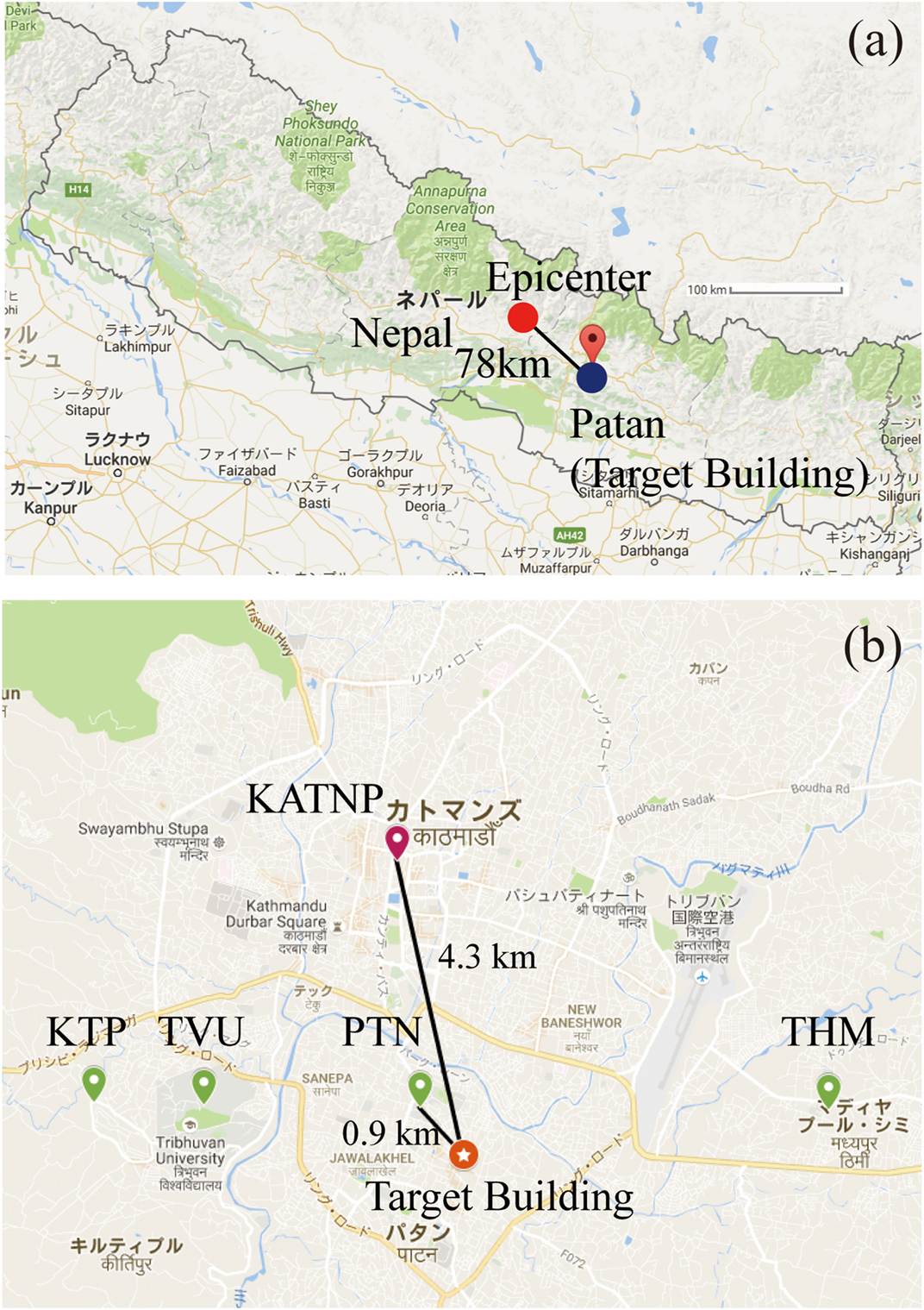
Figure 1. Locations of the epicenter, observation points, and target building (Google Maps, 2016). (A) Location of the epicenter and the target building. (B) Location of the target building and the observation points.

Figure 1B is a map showing the locations of the target building and the observation point at station KATNP, a United States Geological Survey strong-motion station. The distance between the target building and KATNP is about 4.3 km. Acceleration was also observed at four observation stations, KTP, TVU, PTN installed by Takai et al. (2016). The nearest station to the target building is PTN located at a distance of 0.9 km from the target building.

Acceleration Record at KATNP and PTN, and PSHA-Predicted Ground Acceleration

Acceleration Record at KATNP

Figure 2A shows the accelerogram observed at KATNP [Combined Strong-Motion Data (CESMD), 2016]. The peak ground accelerations for the NS, EW, and UD components are 162, 155, and 184 cm/s², respectively.

FIGURE 2

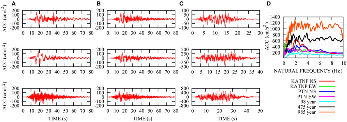
Figure 2. Acceleration record at KATNP and PTN, and probabilistic seismic hazard analysis (PSHA)-predicted ground acceleration (Parajuli et al., 2007; Combined Strong-Motion Data (CESMD), 2016; Takai et al., 2016). (A) Acceleration record at KATNP. (B) Acceleration record at PTN. (C) Synthesized PSHA-predicted ground acceleration for three return periods. (D) Comparison of acceleration response spectra for 5% damping.

Acceleration Record at PTN

Figure 2B shows the accelerogram observed at PTN (Takai et al., 2016). The peak ground accelerations for the NS, EW, and UD components are 151, 128, and 133 cm/s², respectively, which are smaller than those of KATNP.

PSHA-Predicted Ground Acceleration

Figure 2C shows the ground motion accelerogram predicted by the PSHA (Parajuli et al., 2007). The acceleration response spectra for three return periods: 98, 475, and 975 years, were estimated from Nepalese historic seismic data. The envelope function in the time domain was obtained using a regression equation based on the magnitude. The acceleration history was synthesized to match both the acceleration response spectra and envelope functions using random numbers. The return periods of 98, 475, and 975 years are equivalent to the occurrence probabilities of 40, 10, and 5% in 50 years; their peak accelerations are 84, 420, and 630 cm/s², respectively.

Comparison of Acceleration Response Spectra

The acceleration response spectra with a 5% damping ratio for the observed horizontal accelerations at KATNP and PTN, and for the predicted ground accelerations are shown in Figure 2D.

As for the observed accelerations at KATNP, the NS component has the largest peak value of 638 cm/s² at 2.32 Hz and also has a peak value of 398 cm/s² at 0.21 Hz. The EW component has a peak value of 518 cm/s² at 0.22 Hz. A particular feature of this ground acceleration is that the predominant frequency is low.

As for the observed accelerations at PTN, the NS component has the largest peak value of 444 cm/s² at 2.27 Hz. The EW component has the largest peak value of 351 cm/s² at 0.72 Hz. The low frequency contents of PTN are smaller than that of KATNP.

The NS and EW components of the observed accelerations at KATNP and PTN were larger than the predicted ground accelerations with a return period of 98 years, but smaller than the predicted ground accelerations for return periods of 475 or 975 years. The acceleration spectra of the predicted ground motion were almost constant for frequencies from 2 to 10 Hz, while those of the observed accelerations at KATNP and PTN decreases with the increase of frequency from 2 to 10 Hz.

Geometric Characteristics of the Target Building

The target building was built in the seventeenth century. Over its history, it has been damaged by many earthquakes and repaired many times. As shown in Figure 3, the building has the ground floor (GF), the first^t floor (1 F) and the roof floor (RF). The plan dimension of the building is 16.5 m × 5.6 m. The heights of the lower and upper stories are 2.4 and 2.2 m, respectively. The maximum height of the building is 6.5 m. Each wall has openings, with the western wall having the largest openings. The walls are composed of mortared bricks, but the size of bricks varies depending on when and where they were made. The roof consists of corrugated galvanized iron sheets resting on wooden beams and battens.

FIGURE 3

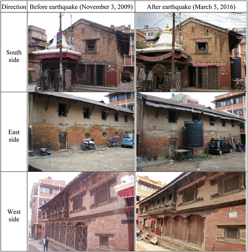
Figure 3. Appearance of building before and after the 2015 Gorkha earthquake.

A plan view of the building is shown in Figure 4. The numbers shown in Figure 4 are the measurement locations, which will be explained in the next section.

FIGURE 4

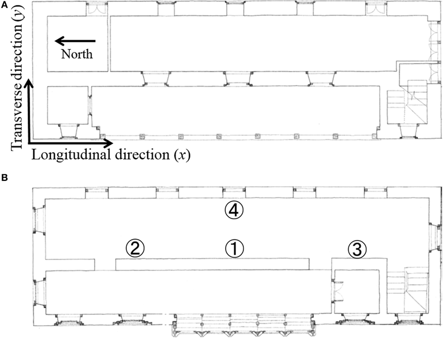
Figure 4. Plan view of the target building with numbered measurement locations. (A) Plan view of the ground floor. (B) Plan view of the upper floor.

Visual Inspection of Structural Damage

Figure 3 shows the comparison of the building appearance from the outside before and after the 2015 Gorkha earthquake. The pictures on the left were taken before the earthquake in November of 2009, and the pictures on the right were taken after the earthquake in March of 2016. Although many minor cracks in mortar were visible during the survey in March of 2016, most of those minor cracks were already present in the photo taken in 2009, and it was difficult to find out new cracks from the outside of the building. Then visual inspection of the cracks inside the building was carried out. Several cracks were found on the both ground and first floors as shown in Figure 5. Although no comparable photos taken prior to the earthquake are present, those cracks appeared to be new. In Figure 5, some walls resemble concrete walls, but they are brick walls covered with plaster. In addition to the cracks shown in Figure 5, several cracks were found on the ceiling of the GF and the timbers were seemingly deteriorated on the RF. Nevertheless, it was difficult to distinguish the damage that already existed before the earthquake through the visual inspection.

FIGURE 5

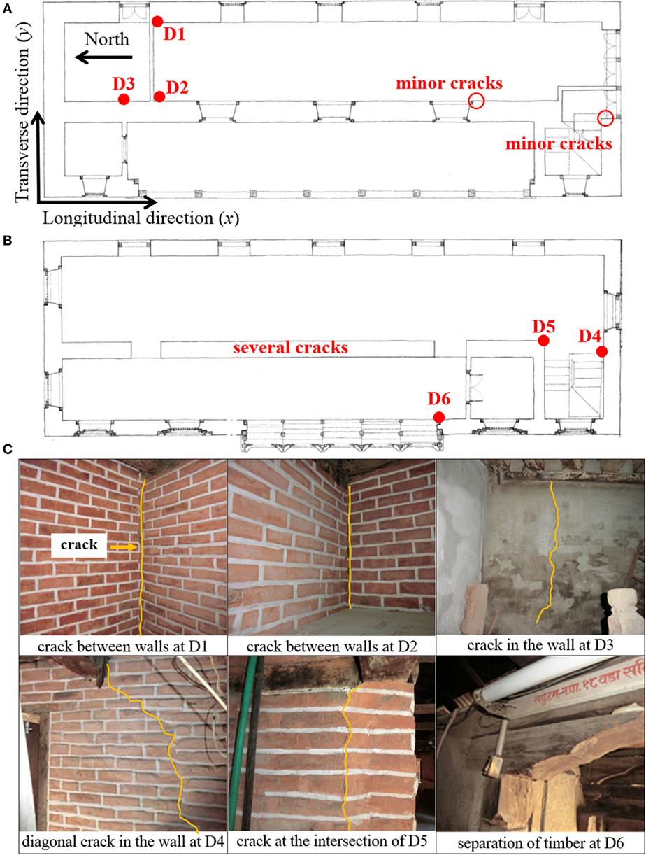
Figure 5. Location and photographs of cracks found in the building after the 2015 Gorkha earthquake. (A) Location of cracks in the ground floor. (B) Location of cracks in the 1st floor. (C) Photographs of cracks found inside the building.

To identify the damage due to the earthquake, microtremor observations were made so that the vibrational characteristics of the building could be compared with those before the earthquake.

Investigation of Vibrational Characteristics Based on Microtremor Observations

Microtremor Observation

Figure 4A shows the layout of the structures and measurement locations where accelerometers were placed. The measurement was conducted at locations 1, 2, and 3 before the earthquake and at locations 1, 2, and 4 after the earthquake as shown in Figure 4B. The measurements at the same locations were not possible due to equipment trouble. The acceleration responses were measured for 10 min in the longitudinal (x, NS) and transverse (y, EW) directions. The sampling interval of measurement data was 0.01 s. The measured waveforms were corrected for baseline and divided into segments of 4,096 data points. 10 sets of 4,096 data points without unsteady portions were extracted manually and the average of their Fourier amplitudes was computed. For smoothing, Parzen window with a frequency band width of 0.4 Hz was applied.

The natural frequencies of the translational vibration modes were determined by the Fourier amplitudes of the first-floor response. The damping ratio of the first mode was also estimated.

By taking the sum and difference of accelerations at locations 1 and 2 in the transverse (y, ES) direction, the transverse vibration was separated into the translational and torsional component.

Result

Natural Frequencies

Figure 6 shows a comparison between the Fourier amplitudes of the responses before and after the earthquake. In each plot, 10 thin lines indicate the Fourier amplitudes of 10 sets of 4,096 data points and one thick line is the average of 10 sets.

FIGURE 6

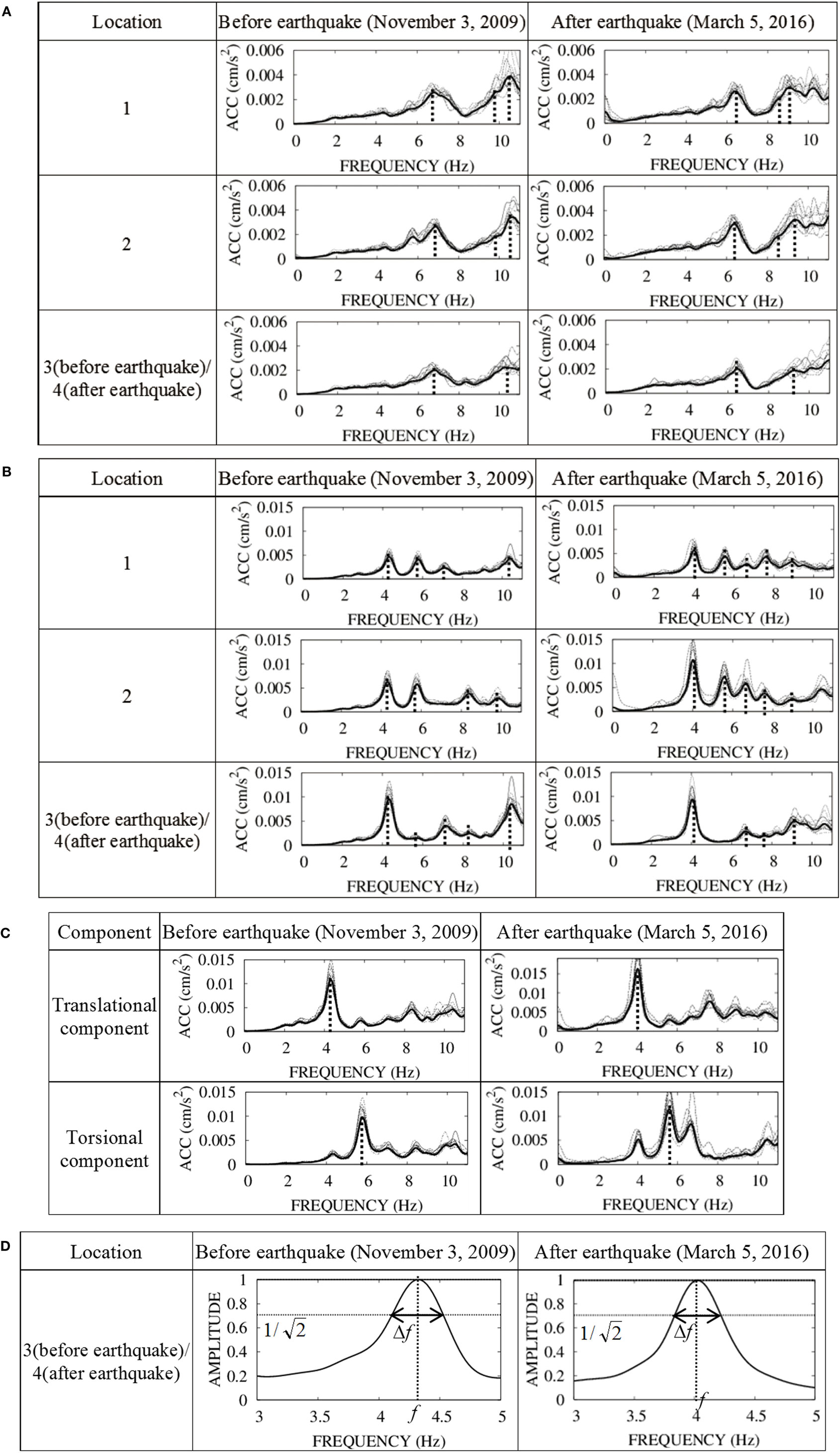
Figure 6. Comparison of ambient vibration of the building before and after the 2015 Gorkha earthquake. (A) Longitudinal (x, NS) direction. (B) Transverse (y, EW) direction. (C) Translational and torsional components in the transverse (y, EW) acceleration. (D) Damping ratio estimation based on the half-power method.

Figure 6A shows a comparison between the Fourier amplitudes of the first-floor responses in the longitudinal (x, NS) direction before and after the earthquake. In Figure 6A, peaks can be seen at around 6.87 and 10.5 Hz before the earthquake and 6.43 and 9.2 Hz after the earthquake. It is reasonable to assume that these frequencies correspond to the natural frequencies of the dominant modes in the longitudinal direction before and after the earthquake. A slight peak can also be seen at locations 1 and 2 around 9.7 Hz before the earthquake and 8.5 Hz after the earthquake.

Figure 6B shows a comparison between the Fourier amplitudes of the first-floor responses in the transverse (y, EW) direction before and after the earthquake. In Figure 6B, peaks can be seen at 4.33, 5.78, 7.13, 8.4, and 10.2 Hz before the earthquake and 4.02, 5.58, 6.68, 7.64, and 9.0 Hz after the earthquake. These frequencies are considered to be the natural frequencies of the modes in the transverse direction. A greater number of the peaks can be seen in the Fourier amplitudes of the response in the transverse direction than that in the longitudinal direction. To further understand these details, the responses were separated into the translational and torsional components.

Figure 6C shows the sum and difference of the Fourier amplitudes at locations 1 and 2 in the transverse (y, EW) direction for pre- and post-earthquake measurements. Because the sum and the difference emphasize the translational motion and the torsional motion, respectively, it is found that the natural frequency of the translational motion is 4.33 Hz before the earthquake and 4.02 Hz after the earthquake. It can also be said that the natural frequency of the torsional mode is 5.78 Hz before the earthquake and 5.58 Hz after the earthquake.

Damping Ratio of the First Mode

The damping ratio of the first transverse mode is calculated by the half-power method under the assumption of white noise excitation. Figure 6D shows the normalized Fourier amplitude around the natural frequency of the first transverse mode. The dashed line indicates an amplitude of $1∕\sqrt{2}$. The damping ratio h is obtained as h = Δf/2f where f is the natural frequency and Δf is the frequency band width shown in Figure 6D. The damping ratios before and after the earthquake are found to be 4.82 and 4.85%, respectively.

Discussion

Comparisons of the natural frequencies of the lowest eight modes and the damping ratios of the first transverse mode are shown in Tables 1 and 2. All of the modes indicate the decrease of the natural frequencies by 3.46 to 11.86% after the earthquake. The structural damage due to the earthquake is evidently shown by the stiffness degradation suggested by this result.

TABLE 1

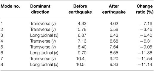
Table 1. Natural frequencies and damping ratio before and after the 2015 Gorkha earthquake: natural frequency.

TABLE 2

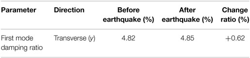
Table 2. Natural frequencies and damping ratio before and after the 2015 Gorkha earthquake: damping ratio of the first mode.

Identification of Structural Parameters and Evaluation of Stiffness Reduction through FEM

General Remarks

In this section, the finite element model of the building is established so that the analytical natural frequencies match the natural frequencies measured before the earthquake. In order to represent the building damaged by the earthquake, the stiffness parameters are calibrated to match the natural frequencies to that measured after the earthquake. The structural damage to the building due to earthquake is identified based on the stiffness change in the finite element model. The computational program of the finite element method, and the stiffness updating technique described in Section “Stiffness Updating Technique Using Natural Frequencies” were developed by authors’ group.

Analysis Model

In the finite element modeling of the building shown in Figure 7, the following assumptions are introduced. The thickness of the brick wall is 60 cm, and the section area of the timber is 15 cm × 15 cm. All components are modeled with 8-node solid elements. The total number of nodes and the elements are 5,674 and 3,128, respectively.

FIGURE 7

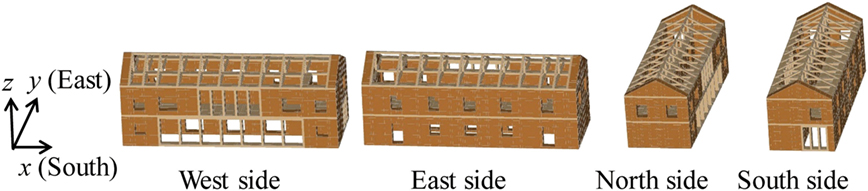
Figure 7. Finite element model of the target building.

The building consists of brick walls, timbers, and a roof. Although the material properties of bricks and mortar are different, the material properties are assumed to be identical. The structural components are classified into nine groups as shown in Table 3. The material properties corresponding to the structural components used in the analysis are also shown in Table 3. They are determined based on the literature regarding the historic masonry building in Nepal. As for timbers, the value used in the analysis of old temples in Nepal was used (Jaishi et al., 2003). As for bricks, the experimental values of bricks taken from old masonry buildings in Nepal was used (Furukawa et al., 2012). Since the ceiling of the GF consists of timber beams and bricks laid on the timber beams, the equivalent density and Young’s modulus are used. The roof itself is not modeled as elements but the effect of the roof weight is included in the density of the timbers in the roof framing.

TABLE 3

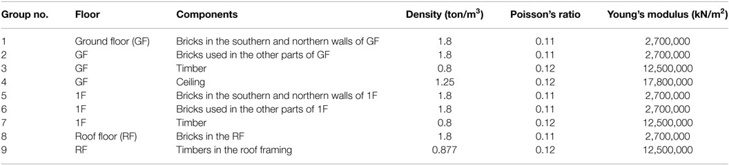
Table 3. Initial finite element model for the building before the earthquake: initial structural parameters of the finite element model for the building before the earthquake.

Comparison of the Observed and Analytical Natural Frequencies

The comparison between the observed natural frequencies and that obtained by the analysis of the initial FE model is shown in Table 4. The natural frequencies of the initial FE model are higher than the observed ones, indicating that the stiffness parameters are overestimated in the initial FE model. One of the possible reasons of the overestimate of the brick stiffness is the overly assumed brick thickness. Although it is assumed in the initial model that the walls are filled with bricks throughout the thickness direction, the actual walls are not likely to be fully filled with bricks and soil-like filler material is included inside. In Figure 8A that shows the middle wall on the first floor taken from the above, soil filler can be seen. The timber stiffness also is overestimated, seemingly due to the deterioration of the material and imperfect connection between members as shown in Figure 8B.

TABLE 4

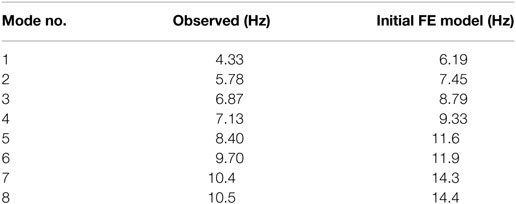
Table 4. Initial finite element model for the building before the earthquake: comparison of observed natural frequencies with the analytical natural frequencies of the initial finite element model for the building before earthquake.

FIGURE 8

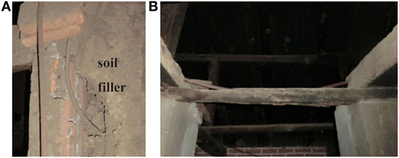
Figure 8. Possible reason of overestimate of stiffness parameters. (A) Soil filled inside the brick wall. (B) Deterioration of timbers and imperfect connection.

Based on the reasoning, the stiffness parameters are updated so that the natural frequencies match the observed ones by means of the procedure to be described in the next section.

Stiffness Updating Technique Using Natural Frequencies

The eigenvalue problem of the baseline finite element model is written as follows:

$\left(-{\mathrm{\lambda }}_i\left[M\right]+\left[K\right]\right)\left\{{\mathrm{\varphi }}_i\right\}=0$ (1)

where [M] is the mass matrix, [K] is the stiffness matrix, λ_i and {ϕ_i} are the i-th eigenvalue and eigenvector, respectively, of the baseline finite element model. The i-th eigenvector λ_i is the square of the natural frequency ω_i.

It is assumed that the exact mass matrix is obtained based on the design document of the prototype structure, and that modeling error only exists in the stiffness matrix. Therefore, the update is applied to the stiffness matrix by [δK] so that the natural frequencies of the updated finite element model match the observed natural frequencies.

The eigenvalue problem of the updated finite element model is expressed as

$\left\{-\left({\mathrm{\lambda }}_i+\mathrm{\delta }{\mathrm{\lambda }}_i\right)\left[M\right]+\left(\left[K\right]+\left[\mathrm{\delta }K\right]\right)\right\}\left(\left\{{\mathrm{\varphi }}_i\right\}+\left\{\mathrm{\delta }{\mathrm{\varphi }}_i\right\}\right)=0$ (2)

where [K] + [δK] is the updated stiffness matrix, δλ_i and {δϕ_i} are the increment of the i-th eigenvalue and eigenvector due to the updating of the stiffness matrix. The i-th eigenvalue and eigenvector of the updated finite element model are λ_i + δλ_i and {ϕ_i} + {δϕ_i}, respectively.

Expanding Eq. 2 and neglecting higher terms yields

$\begin{array}{l}\hfill \left(-{\mathrm{\lambda }}_i\left[M\right]+\left[K\right]\right)\left\{{\mathrm{\varphi }}_i\right\}+\left(-\mathrm{\delta }{\mathrm{\lambda }}_i\left[M\right]+\left[\mathrm{\delta }K\right]\right)\left\{{\mathrm{\varphi }}_i\right\}+\left(-{\mathrm{\lambda }}_i\left[M\right]+\left[K\right]\right)\left\{\mathrm{\delta }{\mathrm{\varphi }}_i\right\}=0\end{array}$ (3)

Since the first term of Eq. 3 becomes 0 from Eq. 1, Eq. 3 becomes

$\left(-\mathrm{\delta }{\mathrm{\lambda }}_i\left[M\right]+\left[\mathrm{\delta }K\right]\right)\left\{{\mathrm{\varphi }}_i\right\}+\left(-{\mathrm{\lambda }}_i\left[M\right]+\left[K\right]\right)\left\{\mathrm{\delta }{\mathrm{\varphi }}_i\right\}=0$ (4)

After multiplication of each term from the left by {ϕ_i}^T, Eq. 4 becomes

${\left\{{\mathrm{\varphi }}_i\right\}}^T\left(-\mathrm{\delta }{\mathrm{\lambda }}_i\left[M\right]+\left[\mathrm{\delta }K\right]\right)\left\{{\mathrm{\varphi }}_i\right\}+{\left\{{\mathrm{\varphi }}_i\right\}}^T\left(-{\mathrm{\lambda }}_i\left[M\right]+\left[K\right]\right)\left\{\mathrm{\delta }{\mathrm{\varphi }}_i\right\}=0$ (5)

Since the mass and stiffness matrices are symmetric, the second term of Eq. 5 becomes

$\begin{array}{l}{\left\{{\mathrm{\varphi }}_i\right\}}^T\left(-{\mathrm{\lambda }}_i\left[M\right]+\left[K\right]\right)\left\{\mathrm{\delta }{\mathrm{\varphi }}_i\right\}={\left\{{\mathrm{\varphi }}_i\right\}}^T\left(-{\mathrm{\lambda }}_i{\left[M\right]}^T+{\left[K\right]}^T\right)\left\{\mathrm{\delta }{\mathrm{\varphi }}_i\right\}\hfill \\ ={\left\{\left(-{\mathrm{\lambda }}_i\left[M\right]+\left[K\right]\right)\left\{{\mathrm{\varphi }}_i\right\}\right\}}^T\left\{\mathrm{\delta }{\mathrm{\varphi }}_i\right\}=0^T\left\{\mathrm{\delta }{\mathrm{\varphi }}_i\right\}=0\hfill \end{array}$ (6)

Therefore, Eq. 5 becomes

${\left\{{\mathrm{\varphi }}_i\right\}}^T\left(-\mathrm{\delta }{\mathrm{\lambda }}_i\left[M\right]+\left[\mathrm{\delta }K\right]\right)\left\{{\mathrm{\varphi }}_i\right\}=0$ (7)

The difference of the eigenvalues can be obtained as

$\mathrm{\delta }{\mathrm{\lambda }}_i=\frac{{\left\{{\mathrm{\varphi }}_i\right\}}^T\left[\mathrm{\delta }K\right]\left\{{\mathrm{\varphi }}_i\right\}}{{\left\{{\mathrm{\varphi }}_i\right\}}^T\left[M\right]\left\{{\mathrm{\varphi }}_i\right\}}$ (8)

The total stiffness matrix [K] is the summation of the element matrices. It is assumed that the elements are classified into n groups, and [K^j] is the summation of all element stiffness matrix belonging to group j ( j = 1, …, n). Then the stiffness matrices are written as

$\left[K\right]={\displaystyle \sum _{j=1}^n}\left[K^j\right]$ (9)

It is assumed that the stiffness error of group j, [δK^j], is proportional to [K^j] with a factor of δk_j.

$\left[\mathrm{\delta }{K}^j\right]=\mathrm{\delta }{k}_j\left[K^j\right]$ (10)

Then, the error in the stiffness matrix [δK] becomes

$\left[\mathrm{\delta }K\right]={\displaystyle \sum _{j=1}^m}\left[\mathrm{\delta }{K}^j\right]={\displaystyle \sum _{j=1}^m}\mathrm{\delta }{k}_j\left[K^j\right]$ (11)

Substituting Eq. 11, Eq. 8 becomes

$\mathrm{\delta }{\mathrm{\lambda }}_i={\displaystyle \sum _{j=1}^n}{A}_{\mathit{ij}}\mathrm{\delta }{k}_j\text{\hspace{0.17em}\hspace{0.17em}where\hspace{0.17em}\hspace{0.17em}}{A}_{\mathit{ij}}=\frac{{\left\{{\mathrm{\varphi }}_i\right\}}^T\left[K^j\right]\left\{{\mathrm{\varphi }}_i\right\}}{{\left\{{\mathrm{\varphi }}_i\right\}}^T\left[M\right]\left\{{\mathrm{\varphi }}_i\right\}}$ (12)

By collecting m eigenvalue differences, δλ_i ( j = 1, …, m), between the observed eigenvalue and the analytical eigenvalue of the baseline model, Eq. 12 becomes a set of m simultaneous equations for n unknowns, δk_j.

The authors developed the computational program of the stiffness updating technique described in this section. The procedure is as follows. First, the total mass matrix [M] and total stiffness matrix [K] of the initial finite element model are obtained. By solving eigenvalue problem of Eq. 1 using [M] and [K], eigenvalue λ_i and eigenvector {ϕ_i} of i-th mode are obtained. Then, element stiffness matrix of the initial finite element model are computed for all elements, and [K^j] is obtained by taking the sum of all element stiffness matrix belonging to group j. A_ij in Eq. 12 is obtained by using [M], [K^j] and {ϕ_i}. δλ_i in Eq. 12 is obtained by taking the difference between the square of observed natural frequencies and analytical eigenvalue λ_i of the initial finite element model. Stiffness change ratio of group j, δk_j, is finally obtained by solving Eq. 12.

Result of Stiffness Updating of the Building before the Earthquake

The elements are divided into 9 groups, namely group Nos.1 to 9 as shown in Table 3. The stiffness error for each group δk_j ( j = 1, …, 9) is obtained by solving Eq. 12. δλ_i (i = 1, …, 8) in Eq. 12 is obtained taking the difference between the square of observed natural frequencies measured before the earthquake and analytical eigenvalue of the initial finite element model. To obtain the solution δk_j of the simultaneous equation expressed by Eq. 12, the Moore–Penrose generalized inverse matrix is used.

The results of the stiffness updating are shown in Tables 5 and 6. The solution of Eq. 12 is stiffness change ratio, δk_j. δk_j is used to update Young’s modulus and stiffness matrix. Young’s modulus E of an element belonging to group j is updated to be E(1 + δk_j). By using the updated Young’s modulus, the stiffness matrix [K] of the updated finite element model is obtained. Natural frequencies of the updated finite element model is obtained by solving the eigenvalue problem of the updated finite element model.

TABLE 5

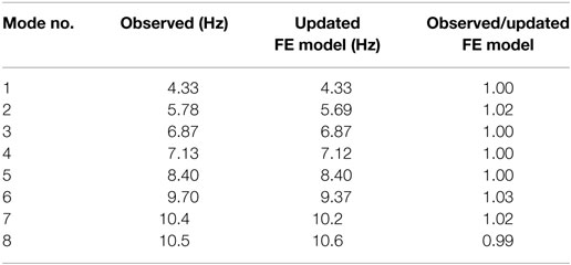
Table 5. Results of stiffness updating for the building before the earthquake: comparison of observed natural frequencies with the analytical ones of the updated finite element model.

TABLE 6

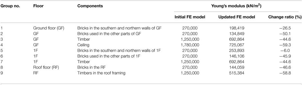
Table 6. Results of stiffness updating for the building before the earthquake: comparison of Young’s modulus between initial and updated finite element model.

Comparison of the natural frequencies of the updated finite element model and that obtained by the measurement before the earthquake are shown in Table 5. They are in good agreement and the validity of the updated finite element model is shown. Table 6 shows the comparison of the initial and updated values of Young’s modulus and stiffness change ratios.

The mode shapes of the eight natural modes are shown in Figure 9. The eigenvector is scaled so that the largest absolute value of its elements be 1.0. Those mode shapes conform to the observed Fourier amplitude spectra shown in Figure 6. For example, the third, sixth, and eighth modes are dominant in the longitudinal (x) direction and other modes are dominant in the transverse (y) direction. In the second mode shown in Figure 9, the phases of the north and south side vibrations are opposite as observed in Figure 6C.

FIGURE 9

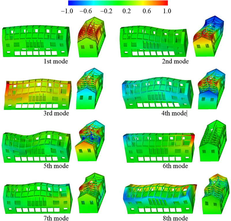
Figure 9. Mode shapes of the lowest 8 modes (Contours in the left and right figures indicate the amplitudes in the longitudinal and transverse directions, respectively).

Result of Stiffness Updating of the Building after the Earthquake and Identification of Stiffness Change

By taking the difference between the square of natural frequencies measured after the earthquake and analytical eigenvalue of the updated finite element model of the building before the earthquake δλ_i (i = 1, …, 8), the stiffness change for each group [δK^j] ( j = 1, …, 9) is obtained.

The stiffness change ratio, δk_j ( j = 1, …, 9), must be larger than −1.0 since the Young’s modulus is positive, and it is natural to assume that the stiffness change ratio of the damaged component is less than 0.0. However, no constraint conditions are considered in solving Eq. 12.

The results of the stiffness updating are shown in Tables 7 and 8. Comparison of the analytical natural frequencies of the updated finite element model and that measured after the earthquake are shown in Table 7. They are in good agreement and the validity of the updated finite element model is shown.

TABLE 7

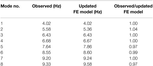
Table 7. Results of stiffness updating for the building after the earthquake: comparison of observed natural frequencies with the analytical ones of the updated finite element model.

TABLE 8

Table 8. Results of stiffness updating for the building after the earthquake: comparison between the values of Young’s modulus in pre-earthquake and post-earthquake finite element models.

The comparison between the values of Young’s modulus of the model before and after the earthquake as well as the stiffness change ratios is shown in Table 8. It is confirmed that the stiffness change ratio is less than 0.0 and larger than −1.0 even though no constraint conditions are considered in solving Eq. 12. It can be seen that the stiffness reduced with factors between 8.0 and 13.8%. The stiffness reduction in the components on the GF is slightly larger than that on the first floor, although the difference is insignificant.

Discussion

The finite element models of the building corresponding to the pre-earthquake and post-earthquake conditions are established by the stiffness updating technique. Building material was divided into nine components, and Young’s modulus of each component is identified so that the analytical natural frequencies match the observed natural frequencies for the building before and after the earthquake. By comparing Young’s modulus before and after the earthquake, it could be seen that the stiffness reduced with factors between 8.0 and 13.8%, indicating the severity of structural damage.

Dynamic Analysis of the Building During Earthquake

Analysis Outline

Dynamic analysis of the building during the Gorkha earthquake was conducted using the pre-earthquake linear finite element building model which was obtained in Section “Result of Stiffness Updating of The building before the Earthquake.” Stiffness proportional damping was used assuming that the first mode damping ratio is 4.82% as shown in Table 2. The NS, EW, and UD components of the ground motion record observed at the nearest PTN station are used as the excitation input in the x(NS), y(EW), and z(UD) directions of the building model.

Although it is likely that structural behavior during the Gorkha earthquake was nonlinear as suggested by the reduced stiffness after the earthquake, a linear analysis was conducted since the nonlinear characteristics necessary for nonlinear analysis is not identified yet. Therefore, the results are used to assess the severity of the response in this study. An integration time interval of 0.005 s is used. Particular attention is made on the acceleration and displacement for reference points, A, B, and C at the top of the GF and the first floor (Figure 10) as the representative responses to describe the computed seismic response of the building. In the future study, the authors would like to identify the nonlinear characteristics of building materials though experiments, and conduct the nonlinear analysis of the building.

FIGURE 10

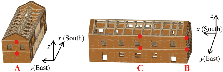
Figure 10. The location of reference points.

Result

Acceleration Response

The acceleration response time histories obtained by the dynamic analysis are shown in Figure 11A (NS component) and Figure 11B (EW component).

FIGURE 11

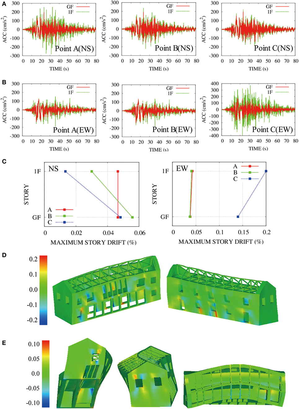
Figure 11. Results of the dynamic analysis. (A) Acecleration response in NS direction. (B) Acecleration response in EW direction. (C) Maximum story drift. (D) Shear strain distribution in the xz-plane at 26 s. (E) Shear strain distribution in the yz-plane at 29 s.

The amplitude of seismic response of Point A on the first floor is significantly greater than that of other points in the NS direction, while the amplitude of the response at Point C is the greatest among all points in the EW direction. It is suggested that the dynamic response of the walls is characterized by the influence of lateral out-of-plane vibration at the center of the wall spans.

Story Drift

The maximum story drifts for the GF and the first floor are shown in Figure 11C.

The maximum story drifts are different depending on the location of the Points A through C. The maximum story drift in EW direction at Point C is the greatest among all. It is suggested that the influence of lateral out-of-plane vibration at the center of the long side wall is significant.

Strain Distribution

The distribution of shear strain of the building model in the xz-plane and yz-plane is shown in Figures 11D,E. The structural deformation is magnified 300 times.

The shear strain in the xz-plane increases up to 0.2 when the building deformation develops in the x direction as shown in Figure 11D. The large shear strain takes place near the corner of the openings in the long side walls.

On the other hand, when the building deformation is in the y direction, significant shear strain of yz-component is observed near the corner of openings in the short side walls as shown in Figure 11E. It is noteworthy that considerable shear strain takes place on both sides of the partition walls on the GF and at the intersection of two inner walls. These parts coincide with the places where actual cracks were found in the post-earthquake inspection of the target building as already shown in Figure 5C. In this section, the distribution of shear strain is selected since it is found that large shear strain takes place where the actual cracks were found in the post-earthquake inspection.

Discussion

It is found that the lateral out-of-plane vibration at the center of the long side wall is significant for the both acceleration response and story drift.

The computed maximum story drift assessed by this simulation using the acceleration at PTN is approximately 0.2% at Point C. The allowable design story drift specified in the provision of the National Building Code of India (Bureau of Indian Standards, 2016) is 0.4%. Considering that the National Building Code is applied in the design of Nepalese buildings, this simulation indicates that the response of the building to the Gorkha earthquake is marginally within the collapse limit state.

The location of structural damage found in the post-earthquake inspection is successfully explained by the shear strain distribution.

Conclusion

A study of a two-story historic masonry building in the Patan district of Kathmandu that survived the 2015 Gorkha earthquake is presented. Since the vibrational characteristics of the building had been measured before the earthquake (in 2009) and microtremor observations were conducted after the earthquake (in 2016), pre- and post-earthquake vibrational characteristics namely natural frequencies and damping ratios are compared.

It was found that the natural frequencies of the lowest 8 modes decreased by 3.46 to 11.86%, indicating structural damage. In a post-earthquake inspection of the building, several cracks were found on the ground and first floors.

The finite element models of the two-story masonry building corresponding to the pre-earthquake and post-earthquake conditions are established, in which the stiffness parameters are identified to match the natural frequencies with the measurement. It could be seen that the stiffness reduced with factors between 8.0 and 13.8%.

Finally, a dynamic analysis of the linear finite element model of the building subjected to the ground motion observed at the PTN station during the Gorkha earthquake was conducted. The locations of structural damage found in the post-earthquake inspection coincide with the area of considerable shear strain developed in the analysis.

Author Contributions

AF carried out the microtremor observation, field survey, vibration data analysis, theoretical formulation development, and numerical analysis. JK carried out the microtremor observation, field survey, and supervised the vibration data analysis. RP and HP carried out the microtremor observation, field survey, and vibration data analysis. KT supervised the vibration data analysis, theoretical formulation development, and numerical analysis.

Conflict of Interest Statement

The authors declare that the research was conducted in the absence of any commercial or financial relationships that could be construed as a potential conflict of interest.

Acknowledgments

The authors deeply thank the late Prof. Hitoshi Taniguchi for his kind encouragement and warming support during our research. The authors express their sincere appreciation to Prof. Akira Igarashi for his valuable comments and guidance in revising the paper.

Funding

Part of the present work was supported by the J-RAPID program of Japan Science and Technology Agency (JST), the Japan Society for the Promotion of Science (JSPS) grant-in-aid (15K06178 and 26249067) and the Grant for Global Sustainability (GGS) initiated by the United Nations University (UNU). These supports are greatly appreciated.

References

Amatya, S. (2008). Monument Conservation in Nepal. Kathmandu: Vajra Publications.

Google Scholar

Bilham, R., and Ambraseys, N. (2005). Apparent Himalayan slip deficit from the summation of seismic moments for Himalayan earthquakes 1500-2000. Curr. Sci. 88, 1658–1663.

Google Scholar

Bureau of Indian Standards. (2016). National Building Code of India. Available at: http://bis.org.in/sf/nbc.htm

Google Scholar

Combined Strong-Motion Data (CESMD). (2016). Earthquakes Recorded by Station KATNP. Available at: http://www.strongmotioncenter.org/cgi-bin/CESMD/StaEvent.pl?stacode=NPKATNP

Google Scholar

Disaster Preparedness Network Nepal. (2016). Earthquake. Available at: http://www.dpnet.org.np/index.php?pageName=earthquake

Google Scholar

Dumaru, R., Rodrigues, H., Furtado, A., and Varum, H. (2016). Seismic vulnerability and parametric study on a bare frame building in Nepal. Front. Built Environ. 2:31. doi: 10.3389/fbuil.2016.00031

CrossRef Full Text | Google Scholar

Furukawa, A., Kiyono, J., Taniguchi, H., Toki, K., Tatsumi, M., and Parajuli, H. R. (2012). Detailed modeling and seismic behavior analysis of existing historic masonry building in Patan District, Kathmandu Valley, Nepal. J. Disaster Mitig. Cult. Heritage Hist. Cities 6, 53–60.

Google Scholar

Goda, K., Kiyota, T., Pokhrel, R. M., Chiaro, G., Katagiri, T., Sharma, K., et al. (2015). The 2015 Gorkha Nepal earthquake: insights from earthquake damage survey. Front. Built Environ. 1:8. doi:10.3389/fbuil.2015.00008

CrossRef Full Text | Google Scholar

Google Maps. (2016). Available from: https://www.google.co.jp/maps?hl=ja

Google Scholar

Jaishi, B., Ren, W., Zong, Z. H., and Maskey, P. N. (2003). Dynamic and seismic performance of old multi-tiered temples in Nepal. Eng. Struct. 25, 1827–1839. doi:10.1016/j.engstruct.2003.08.006

CrossRef Full Text | Google Scholar

National Planning Commission. (2015). Government of Nepal, Post Disaster Needs Assessment, Vol. A: Key Findings. Kathmandu: Print Communication Pvt. Ltd.

Google Scholar

Parajuli, H. R., Kiyono, J., Ono, Y., and Tsutsumiuchi, T. (2007). Design earthquake ground motions from probabilistic response spectra: case study of Nepal. J. Jpn. Assoc. Earthq. Eng. 8, 16–28. doi:10.5610/jaee.8.4_16

CrossRef Full Text | Google Scholar

Parajuli, H. R., Kiyono, J., Taniguchi, H., Toki, K., Furukawa, A., and Maskey, P. M. (2010). Parametric study and dynamic analysis of an historical masonry building of Kathmandu. J. Disaster Mitig. Cult. Heritage Hist. Cities 4, 149–156.

Google Scholar

Parajuli, H. R., Kiyono, J., Tatsumi, M., Suzuki, Y., Umemura, H., Taniguchi, H., et al. (2011). Dynamic characteristic investigation of an historical masonry building and surrounding ground in Kathmandu. J. Disaster Res. 6, 26–35. doi:10.20965/jdr.2011.p0026

CrossRef Full Text | Google Scholar

Parajuli, R. R., and Kiyono, J. (2015). Ground motion characteristics of the 2015 Gorkha Earthquake, Survey of damage to stone masonry structures and structural field tests. Front. Built Environ. 1:23. doi:10.3389/fbuil.2015.00023

CrossRef Full Text | Google Scholar

Rana, B. S. J. R. (1935). Nepal’s Great Earthquake 1934. Tripureshwor, Kathmandu (in Nepali): Sahayogi Press.

Google Scholar

Rohit, K. R. (2007). Heritage Homeowner’s Preservation Handbook. Bangkok: UNESCO.

Google Scholar

Takai, N., Shigefuji, M., Rajaure, S., Bijukchhen, S., Ichiyanagi, M., Dhital, M. R., et al. (2016). Strong ground motion in the Kathmandu Valley during the 2015 Gorkha, Nepal, earthquake. Earth Planets Space 68, 1–8. doi:10.1186/s40623-016-0383-7

CrossRef Full Text | Google Scholar