Comparing Structural Identification Methodologies for Fatigue Life Prediction of a Highway Bridge

1. Introduction

In this paper, four data-interpretation methodologies for model updating are compared to evaluate their applicability in predicting the remaining fatigue life of a full-scale bridge. The deficit between demand and supply of civil infrastructure is increasing annually from an estimated US$ 1 trillion in 2014 (World Economic Forum, 2014). Performance-based asset management of existing infrastructure for decisions such as repair and retrofit for life extension helps reduce this deficit. Replacement of all aging infrastructure is expensive, unsustainable, and often not necessary. Models that are used for design of civil infrastructure are justifiably conservative. Therefore, most structures possess reserve capacity and can last well beyond their design working lives (referred to as service lives in this paper) (Brühwiler, 2012; Smith, 2016). The challenge lies in quantifying this reserve capacity to enable asset-management decision making such as repair, retrofit, and extension.

Asset-management decision making may be improved through a better understanding of structural behavior. This can be achieved through monitoring of civil infrastructure enabled by recent advances in sensing technology (Lynch and Loh, 2006; Taylor et al., 2016) and availability of affordable computational tools (Frangopol and Soliman, 2016). However, analytical models of civil infrastructure systems possess large modeling uncertainty, including significant systematic errors and unknown correlations between measurement locations (Jiang and Mahadevan, 2008). These conditions have lead to recent studies of uncertainties and development of data-interpretation methodologies that are robust to incomplete knowledge (Goulet and Smith, 2013). Moreover, civil infrastructure are in service for decades and are subjected to changing load and environmental conditions. Therefore, data-interpretation methodologies should support engineers for iterative asset-management decisions as new information becomes available throughout infrastructure lives.

Structural identification involves interpreting measurement data to update knowledge of parameters governing structural response in the presence of uncertainties from numerous sources. Methodologies for structural identification have been studied extensively (Worden et al., 2007; Beck, 2010; Cross et al., 2013; Moon and Catbas, 2013). However, every civil structure is unique due to its form, function, and utility and this requires explicit consideration of uncertainties in decision making. Most data-interpretation methodologies assume that the uncertainty associated with the structural system is defined by a zero-mean independent Gaussian distribution. However, this assumption is rarely satisfied for civil infrastructure (Pasquier et al., 2014). Lack of knowledge of uncertainty related to aspects such as geometry of structural elements and model bias means that most sources can only be estimated as bounds. There are other sources of uncertainties, such as support conditions, that are systematic in nature and their magnitudes may change the correlation between uncertainties at measurement locations. Misevaluation of these uncertainties have led to incorrect updated probability distributions (Goulet and Smith, 2013; Simoen et al., 2013; Pasquier and Smith, 2015). Such inaccuracy can result in misinformed asset-management decisions.

The success of data-interpretation methodologies is best measured on full-scale examples. Brownjohn et al. (2011) have noted difficulties in transfer of technology from the laboratory to the field. Laboratories, by design, are intended to reduce uncertainty and thus they provide little similitude with structural identification of real structures. Unfortunately, there are many studies and theoretical proposals found in the literature (Ben-Haim and Hemez, 2012) that have not involved testing with full-scale systems. Yan and Katafygiotis (2015) have presented a novel approach for Bayesian model updating and highlighted the difficulties in implementing the procedure in engineering practice. They assert that the number of parameters to be identified and the large uncertainty associated with complex systems may lead to an unidentifiable system, requiring the need for model reduction techniques. Kuok and Yuen (2016) have studied modal identification of the Ting Kau Bridge, which is monitored with more than 230 sensors of various types. They employ a Bayesian framework for parameter estimation and model class selection. Their study shows that the identification results obtained are influenced by monitoring conditions such as wind. Behmanesh and Moaveni (2016) have carried out hierarchical Bayesian model updating of a footbridge that is subjected to varying temperature conditions. They consider the effect of parameter uncertainty, parameter variability due to ambient or environmental conditions and modeling error uncertainty for continuous monitoring. The results from their study show the importance of including modeling errors for response prediction. There is a continuing need to evaluate applicability of model updating methodologies to full-scale systems under practical conditions.

Detailed numerical models have been used to capture the physical conditions affecting the response of a full-scale system. Use of these models in data-interpretation methodologies was recognized to be computationally expensive (Chang et al., 2000). Surrogate models have been proposed to improve computation times. Surrogate models that replaced finite-element models include polynomial regression (Hemez et al., 2002), multivariate regression spines (Friedman, 1991), and Kriging estimates (Simpson et al., 2001) as reviewed by Rutherford et al. (2006). Worden and Cross (2018) presented the utility of using surrogate models to predict bridge response under the influence of environmental conditions such as temperature. Support vector machines have been used for predicting correlation between modal frequencies and temperature (Ni et al., 2005), fatigue truck load model (Lu et al., 2016), and to obtain bridge scour information (Chou and Pham, 2017). A back propagation neural network model was used by Ni et al. (2009) to model the correlation between model frequencies and temperature of the Ting Kau bridge. In this paper, neural network models have been used to obtain the structural response for both identification and prediction.

Most research so far has focused on parameter identification primarily for the purpose of damage detection. Few researchers have aimed to predict structural response for asset-management decision making. Li et al. (2016) have predicted von Mises stress in a test structure. They have employed a Bayesian framework to arrive at a posterior distribution of model parameters, which they then utilized to predict von Mises stress at an unmeasured location. Their study has found that there is a large uncertainty associated with prediction. Therefore, the forward problem of prediction requires rigorous treatment of uncertainty associated with the system. This research exemplifies the need for uncertainty quantification utilizing engineering knowledge to enable robust prediction of structural response for the purpose of asset-management decision making.

Pasquier and Smith (2015) compared a model falsification-based methodology and Bayesian model updating under various uncertainty conditions for prediction utilizing a simple beam. Their results showed that the model falsification methodology provided accurate prediction in presence of non-Gaussian sources of uncertainty, model bias, and other sources of systematic uncertainty. Based on this observation, Pasquier et al. (2014) and Pasquier et al. (2016) utilized model falsification for reserve capacity estimation of a full-scale bridge. However, no research was found that compares several data-interpretation methodologies for reserve capacity estimation on a full-scale case study.

This paper compares four data-interpretation methodologies, residual minimization (Alvin, 1997), traditional Bayesian model updating (BMU) (Beck and Katafygiotis, 1998), error-domain model falsification (EDMF) (Goulet and Smith, 2013), and a modified formulation of BMU. These methodologies are briefly explained in Section 2. The objective of this comparison is to verify the applicability of these methodologies for use in practice for the purpose of reserve capacity estimation. They are compared based on their ability to provide robust identification and prediction for a full-scale structure in presence of systematic uncertainty and incomplete correlation information. Also, these methodologies have been evaluated based on their compatibility with introduction of new information, ease of understanding for use in practice, and computation demand. Using updated information, the remaining fatigue life of the bridge is predicted under two traffic loading scenarios observed using a weigh-in-motion (WIM) station and one simulated future loading scenario.

2. Background—Methodologies for Data-Interpretation

In this section, a brief explanation of four data-interpretation methodologies, residual minimization, traditional BMU, EDMF, and modified BMU is presented. Residual minimization is a deterministic methodology, while EDMF and BMU are probabilistic methodologies that can incorporate multiple sources of uncertainty associated with the system. These methodologies differ in the assumptions that are made to represent the uncertainty associated with the system.

2.1. Residual Minimization

In residual minimization, a structural model is calibrated by determining model parameter values that minimize the error between model prediction and measurements. Sanayei et al. (2011) presented a manual model updating example where model predictions are manually compared to measurements and the model is calibrated based on engineering knowledge to minimize an objective function. A typical objective function for residual minimization is shown in equation (1):

$\widehat{\theta }=\begin{array}{c}\hfill \mathit{argmin}\hfill \\ \hfill \mathrm{\theta }\hfill \end{array}{\displaystyle \sum _{i=1}^{n_y}}{\left(g\left(x_i,\mathrm{\theta }\right)-{ŷ}_i\right)}^2.$ (1)

In equation (1), $\widehat{\theta }$ is the optimum model parameter set obtained using measurements, $\left(g\left(x_i,\mathrm{\theta }\right)-{ŷ}_i\right)$ is the residual obtained between the model response, $g\left(x_i,\mathrm{\theta }\right)$, and measurement, ${ŷ}_i$, at measurement location i. Residual minimization does not account for the inherent model bias in civil infrastructure due to application of safe design models. It also does not take into account uncertainties arising from systematic or environmental sources and the correlation between uncertainties. The simplicity of the methodology makes it popular for use in practice, although the identification results obtained are not always accurate (Beven, 2000).

2.2. Traditional Bayesian Model Updating

Bayesian model updating is a popular methodology for structural identification. In this methodology, prior knowledge of model parameters is updated using information obtained through monitoring of a structure. If g(θ) is the model of a structure with parameters θ, then the prior probability distribution function (PDF) of the model parameters, P(θ) is updated as shown in equation (2),

$P\left(\mathrm{\theta }|y\right)=\frac{L\left(y|\mathrm{\theta }\right)\cdot P\left(\mathrm{\theta }\right)}{L\left(y\right)}$ (2)

where P(θ|y) is the posterior or updated PDF of model parameters, L(y|θ) is the likelihood function, and L(y) is the normalizing constant. The likelihood function, L(y|θ), indicates the plausibility of observing data y for a given realization of θ.

In traditional BMU methodology (Beck and Katafygiotis, 1998), a L₂-norm-based Gaussian likelihood function, as shown in equation (3), is used to update prior information of model parameters:

$L\left(y|\mathrm{\theta }\right)=2{\mathrm{\pi }}^{-n_m/2}{\left|\Sigma \right|}^{-1/2}\mathit{exp}\left[{\left(-\frac{1}{2}{\mathrm{\epsilon }}_0\left(\mathrm{\theta }\right)-U_c\right)}^T\times {\Sigma }^{-1}\left(-\frac{1}{2}{\mathrm{\epsilon }}_0\left(\mathrm{\theta }\right)-U_c\right)\right].$ (3)

In equation (3), Σ is the correlation matrix defined by the correlation coefficients between measurement locations, ε₀(θ) is a vector of residuals between observation and model response, and U_c is a vector containing the mean of uncertainty at each measurement location.

In traditional BMU, the uncertainty associated with the system is assumed to have an independent zero-mean Gaussian distribution implying model bias and correlations are not considered. A prominent approach to account for model bias is to model it as a Gaussian process with variance σ² (Kennedy and O’Hagan, 2001), which is assigned a non-informative prior and whose posterior distribution is identified along with other model parameters. Brynjarsdóttir and O’Hagan (2014) used an informed prior for σ² to include available information about the model error. Although these approaches provided reliable estimates of model parameters in a few cases, they failed to provide reliable solutions for extrapolation (prediction at an unmeasured location). In the context of civil infrastructure, some researchers have considered modeling uncertainty for updating response prediction (Papadimitriou et al., 2001), fatigue reliability assessment (Kwon et al., 2010), and damage assessment (Simoen et al., 2015). In the above studies, modeling uncertainty at all measurement locations is assumed to be the same, which is rarely the case in the presence of systematic bias. Also, Bayesian methodology may provide accurate identification of parameters at measured locations but the information obtained from measurements cannot be extrapolated to predict structural responses at other locations in the presence of systematic bias (Behmanesh et al., 2015; Pasquier and Smith, 2015).

2.3. Error-Domain Model Falsification

Another methodology for model updating is EDMF (Goulet and Smith, 2013). In this methodology, information from measurements is used to falsify parameter values, thereby obtaining a candidate set from an initial set of possible parameter values. This methodology is based on the assertion by Popper (1959) that models cannot be validated by data; they can only be falsified. Conservative and simplified models used to design civil infrastructure possess model bias, model fidelity uncertainty, and uncertainties from simplification of loading conditions, geometrical properties, material properties, and boundary conditions. Most of these uncertainties can be estimated only using engineering heuristics and cannot be described using a zero-mean Gaussian distribution. In EDMF, engineering knowledge is utilized to quantify uncertainties from various sources and combined together along with measurement uncertainty to obtain a robust falsification criterion.

Consider a structure with modeling and measurement uncertainty, at a measurement location i, ${\mathrm{ϵ}}_{\mathit{mod},i}$, and ${\mathrm{ϵ}}_{\mathit{meas},i}$, respectively. If a structure is represented by a physics-based model, g(θ), then the true response of the structure at a measurement location, Q_i, is given by,

$Q_i=g_i\left({\mathrm{\theta }}^{\ast }\right)+{\mathrm{ϵ}}_{\mathit{mod},i}$ (4)

where g_i(θ*) is the model response at measurement location i for the real values of the model parameters, θ* and ${\mathrm{ϵ}}_{\mathit{mod},i}$ are the modeling uncertainty at the measurement location. Similarly, if the structure is monitored, then the true response of the structure at a measurement location, Q_i, is given by,

$Q_i=y_i+{\mathrm{ϵ}}_{\mathit{meas},i}$ (5)

where y_i is the measured response of the structure and ${\mathrm{ϵ}}_{\mathit{meas},i}$ is the measurement uncertainty at the measurement location. Equating equations (4) and (5), the following relationship between model response and measurement can be obtained,

$g_i\left({\mathrm{\theta }}^{\ast }\right)-y_i={\mathrm{ϵ}}_{\mathit{meas},i}-{\mathrm{ϵ}}_{\mathit{mod},i}$ (6)

where the residual between model response and measurement at a sensor location is equal to the combined model and measurement uncertainty. In design decision making, an important consideration is to first fix a target reliability for design. Therefore, in using EDMF for asset-management decision making, first a target reliability of identification, ϕ ∈ {0,1}, is established (Goulet and Smith, 2013). Using the target reliability for identification, the criteria for falsification in EDMF, thresholds T_high,i and T_low,i, are computed using equation (7):

${\mathrm{\varphi }}^{1/m}={\displaystyle \underset{T_{\mathit{low},i}}{\overset{T_{\mathit{high},i}}{\int }}}{f}_{U_{c,i}}\left({\mathrm{ϵ}}_{c,i}\right)d{\mathrm{ϵ}}_{c,i}.$ (7)

In equation (7), $f_{U_{c,i}}\left({\mathrm{ϵ}}_{c,i}\right)$ is the combined uncertainty PDF at measurement location i and ϕ is the target reliability of identification. The combined uncertainty, $f_{U_{c,i}}\left({\mathrm{ϵ}}_{c,i}\right)$, is calculated by combining uncertainty from various sources such as geometric simplifications, modeling assumptions, and sensor resolutions using Monte Carlo sampling. If the target reliability of identification, ϕ, is set to 0.95, then using Monte Carlo sampling, 1 million samples from the combined uncertainty distribution are generated. From these samples, the smallest range that contains 95th percentile of the samples is calculated. The bounds of this range correspond to the threshold bounds, T_high,i and T_low,i. In equation (7), the term 1/m is the Šidák correction (Šidák, 1967) that accounts for a finite number of measurements m. For example, using Šidák correction, if the desired target reliability of identification is 0.95 using two measurements, then the thresholds bounds are computed for 97.5th percentile (0.95^1/2) of the generated samples. Once, the bounds, T_high,i and T_low,i, are computed, the user generates model responses for various instances of model parameters, θ. If the residual between model prediction and measurement does not lie within the thresholds then the model instance is falsified as shown in equation (8):

$T_{\mathit{low},i}\le g_i\left(\mathrm{\theta }\right)-y_i\le T_{\mathit{high},i}\forall i\in \left\{1...n_m\right\}.$ (8)

Using equation (8), if the response of a model instance does not lie within the established thresholds for any measurement location, then that model instance is falsified (Goulet et al., 2010, 2013b; Goulet and Smith, 2013). The remaining model instances from the initial set, whose responses for all measurement locations lie within the thresholds are accepted to form the candidate model set. These candidate models are then utilized to carry out model prediction with reduced uncertainty (Pasquier and Smith, 2015).

The EDMF methodology has been developed and applied to fourteen full-scale systems since 1998 (Smith, 2016). Recent applications include model identification (Goulet et al., 2013b), leak detection (Goulet et al., 2013a; Moser et al., 2015), wind simulation (Vernay et al., 2015), prediction (Pasquier and Smith, 2016), fatigue life evaluation (Pasquier et al., 2014, 2016), and measurement system design (Goulet and Smith, 2012a,b; Papadopoulou et al., 2016).

2.4. Modified Bayesian Model Updating

The other methodology considered for comparison in this paper is the modified BMU. In this methodology, prior knowledge of model parameters is updated using measurements as shown in equation (2). However, a box-car-shaped L_∞-norm-based Gaussian likelihood function is used to include information gained through measurements. A generalized Gaussian distribution is defined as,

$f\left(x,k\right)=\frac{{\mathrm{\kappa }}^{1-1/\mathrm{\kappa }}}{2{\mathrm{\sigma }}_{\mathrm{\kappa }}\mathrm{\Gamma }\left(1/\mathrm{\kappa }\right)}{e}^{\mathrm{\kappa }\cdot {\left[\frac{\left|x-x_0\right|}{{\mathrm{\sigma }}_{\mathrm{\kappa }}}\right]}^{\mathrm{\kappa }}}$ (9)

where f(x, κ) is the generalized Gaussian PDF of random variable x, based on L_κ-norm with mean, x₀, and SD, σ_κ. For κ → ∞, f(x, κ) tends to a box-car shape. Parameters, x₀ and σ_κ, of the likelihood function are determined using threshold bounds from equation (7) as shown in equations (10) and (11):

$x_0=\frac{T_{\mathit{high},i}-T_{\mathit{low},i}}{2}$ (10)

${\mathrm{\sigma }}_{\mathrm{\kappa }}=T_{\mathit{high},i}-x_0.$ (11)

The L_∞-norm-based Gaussian likelihood function is approximated using κ = 200. If the residuals between model response and measurements at all locations lie within the thresholds, then that model instance is attributed a higher likelihood of occurrence, while model instances that would be falsified in EDMF are attributed a low likelihood. The application of modified BMU was compared with traditional BMU and EDMF, using an illustrative example, by Pai and Smith (2017).

In this paper, these four methodologies are compared considering a range of uncertainty sources and computational demands of simulating the behavior of a full-scale structure. Results obtained from model updating are utilized for fatigue life evaluation of a full-scale bridge under two traffic loading scenarios.

3. Case Study

3.1. Structure Description

The case considered here is inspired from a steel–concrete composite highway twin bridge in the town of Echandens, Switzerland, called the Venoge bridge. The bridge has four spans of length 52, 60.4, 55, and 52 m, and a total length of 219.4 m. In 1995, the bridge was extended from 2 × 2 lanes to 2 × 3 lanes by adding an additional lane in each traffic direction. The bridge is part of the European route E62 and on average, 7,008 heavy vehicles cross the bridge weekly in one direction with an average weight of 22 tons. According to Eurocode, the term heavy vehicles refers to vehicles with weight greater than 10 tons (Eurocode, 1991). Most of these heavy vehicles drive on the slow lane on the extended part of the bridge as shown in Figure 1.

FIGURE 1

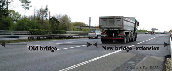
Figure 1. Venoge bridge (Credit: IMAC, EPFL).

Each half of the twin bridge is composed of a concrete deck supported over four steel girders. The extended lane and the old bridge in one traffic direction are supported by two steel girders each. The concrete bridge deck and steel girders under the extended lane are modeled using SHELL182 elements in ANSYS. The steel girders supporting the old bridge are modeled using BEAM188 elements. The finite-element model is used for a linear elastic analysis in which the deck is assumed to be homogeneous and un-cracked on supports under fatigue loads. The bridge has four spans as shown schematically in Figure 2. The bridge is monitored using ten strain gages, installed in 1995, located at two sections along the span as shown in the figure. These sensors are located on the interior girder supporting the extended lane of the bridge. Supports Sup 0, Sup 1, and Sup 2, supporting the extended lane of the bridge are modeled using spring elements with parametrized stiffness. Sup 3, Sup 4, and supports under the old bridge are modeled using rigid spring elements.

FIGURE 2

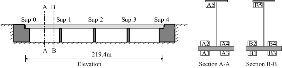
Figure 2. Sensor locations on the Venoge bridge.

Sensors, A1 to A4 and B1 to B4, are used for updating parameters of the model. Using this updated knowledge, the response at sensor locations, A5 and B5, is predicted for validation of the results obtained using the data-interpretation methodologies. The updated model parameters are then used to predict the remaining fatigue life of a cover plate detail on the bridge. This cover plate detail is located near sensors A1 and A3, shown in Figure 2. In this study, the minimum remaining fatigue life of the bridge for this critical detail is evaluated using in-service traffic and strain measurement data. The number of sensors and their location on the bridge is sub-optimal. The measurement system was installed in 1995 for another objective than the one being studied in this paper.

3.2. Measurement and Traffic Load Data

Figure 2 shows the position of the sensors on the inner girder of the extended section of the bridge. Data from eight sensors, A1 to A4 and B1 to B4, are used for updating knowledge of the bridge behavior. The position of sensors B1 and B3 on the bridge is shown in Figure 3. Four sensors are located close to the location of the critical detail and four other sensors are located at the end of the first span, 1 m from the support, Sup 1. Data from these eight sensors, recorded from November 18 to 24, 2013, is used for identification of the model parameters. However, as the data available is a time-history, it has to be processed to acquire a response that can be utilized for data-interpretation. A comparable structural response is the equivalent stress range. The equivalent stress range calculated using in-service strain measurements is considered as measured response at sensor locations, y_i. The computation of equivalent stress range is explained in Section 3.3.

FIGURE 3

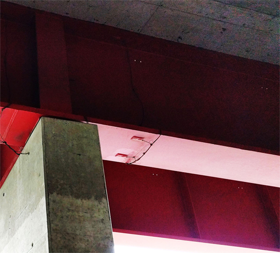
Figure 3. Sensors B1 and B3 on the Venoge bridge (Credit: IMAC, EPFL).

The traffic load on the bridge from November 18 to 24, 2013, in the direction Lausanne–Geneva, is obtained from a weigh-in-motion (WIM) station located only 1 km from the bridge, at Denges, without any exits in between. The WIM station provides traffic load in terms of time of passage (T), vehicle speed (V), number of axles (N), total length (TL), gross total weight (GTW), axle weight (AW), and distance between axles (AD). Using this traffic data, a train of axle loads is generated for the 1-week duration from November 18 to November 24, 2013. This axle train is used as a moving point load on the bridge to obtain the equivalent stress range at each sensor location.

3.3. Computation of Equivalent Stress Range and Remaining Fatigue Life

Each sensor shown in Figure 2 provides a time-history of strain for vehicles passing over the bridge. This time-history of strain is used to compute the stress range histogram using the rainflow algorithm (Matsuishi and Endo, 1968). In the stress range histogram, stress range values below 2 MPa are not considered due to their low effect on fatigue damage of the bridge. The equivalent stress range, Δσ_e (Dowling, 1971), is computed using equation (12),

$\mathrm{\Delta }{\mathrm{\sigma }}_e={\left[\sum \frac{n_i\mathrm{\Delta }{\mathrm{\sigma }}_i^m}{\sum n_i}\right]}^{1/m}$ (12)

where n_i is the number of cycles that takes place at stress range level Δσ_i and m is the slope coefficient of the S–N curve. The equivalent stress range is calculated using a single slope S–N curve, which is a conservative assumption.

Similarly, the equivalent stress range is computed for each model instance using the finite-element model and traffic load on the bridge. The finite-element model is used to generate an influence line for stress at each sensor location for a given set of parameter values. The train of axle loads is passed over influence line of each sensor and processed using the rainflow algorithm to obtain stress range histograms. The equivalent stress range is computed from these histograms using equation (12) for all sensors. This step is repeated to obtain the equivalent stress range at each sensor location for various model parameter values.

The updated model using traffic and strain data is used to predict the remaining fatigue life of a cover plate detail located close to sensors, A1 and A3, as shown in Figure 2. The remaining fatigue life of the cover plate detail is computed using the damage index. The damage index, D_period, is calculated using Miners rule (Miner, 1945), as shown in equation (13):

$D_{\mathit{period}}=\left[\sum \frac{n_i}{C\cdot \mathrm{\Delta }{\mathrm{\sigma }}_i^{-m}}\right]$ (13)

where C is a constant depending on the category of the critical detail, m is the slope coefficient, and n_i is the number of cycles that takes place at stress range level Δσ_i. The cover plate welded attachment close to sensor A1 and A3 is classified as FAT36 according to SIA263/1 (2013). Based on the detail classification, the characteristic value for the constant C is utilized in computing the damage index. The remaining fatigue life of the bridge, RFL, is calculated using equation (14):

$\mathit{RFL}=\frac{R_{\mathit{year}}}{D_{\mathit{period}}}$ (14)

where R_year is the fraction of traffic simulation period over a year. Thus, if traffic is simulated over a 1-week period, then R_year is taken as 1/52.

3.4. Model Class and Sources of Uncertainty

The bridge response, i.e., the equivalent stress range at the sensor locations, is affected by several factors, which are not known completely. In the finite-element model, unknown parameters are quantified as random variables with a uniform distribution. Not all parameters of the finite-element model affect the structural response significantly. The relative importance of these parameters to structural response is estimated using a sensitivity analysis. Equivalent stress range at each sensor location is calculated for numerous values of model parameters. The dataset containing the model response and parameters is used to fit a linear regression model for each sensor location. The parameters of the regression model are indicative of the importance of the structural parameters to response at each sensor location, which is used to calculate the relative importance. A list of these parameters is shown in Table 1 along with their relative importance to the structural response of the bridge at various sensor locations.

TABLE 1

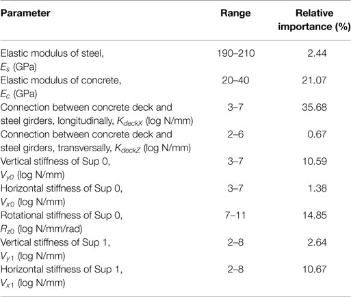
Table 1. Parametric uncertainty.

The parameters that significantly affect the structural response based on their relative importance are E_c, K_deckX. These parameters constitute the parameters of the model class and knowledge regarding these parameters will be updated using data from strain gages and WIM station. The parameters not considered in the model class for the identification are called as secondary parameters. They contribute to the secondary parameter uncertainty at each sensor location, which is estimated using the finite-element model. The secondary parameter uncertainty at each sensor location is shown in Table 2.

TABLE 2

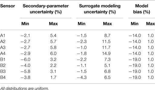
Table 2. Secondary parametric uncertainty, surrogate modeling uncertainty, and model bias at each sensor location.

Probabilistic data-interpretation methodologies, such as those discussed in Section 2, require evaluation of a structural model for various realizations of model parameters, which are described as random variables. In this paper, a finite-element model of the bridge is used as the structural model with two parameters, E_c, K_deckX, comprising the model class to be identified. Each realization of the model parameters is a set of values for E_c, K_deckX for which the bridge response is evaluated. Using the finite-element model and a realization of the model parameters, an influence line for stress at each sensor location is obtained. This influence line is then used to obtain the equivalent stress range at each sensor location. The computation of influence line for all sensors for one set of model parameters takes around 4 h and 30 min, using an Intel(R) Xeon(R) CPU E5-2670 v3 @2.30GHz processor. The long computation does not allow for efficient sampling of the parameter space to obtain optimum results. Therefore, to reduce the computation cost, surrogate models are developed to predict the equivalent stress range at each sensor location and the remaining fatigue life of the critical detail. The equivalent stress range predicted using the surrogate models for various parameter values is taken to be the model response, g_i(θ), in model updating.

120 parameter values of E_c, K_deckX are generated using Latin hypercube sampling and input into the finite-element model to obtain the equivalent stress range at sensor locations and remaining fatigue life of the critical detail. The parameter values and the corresponding structural response obtained are used as a data set to train the surrogate models. Here, a neural network is used to map the function between the inputs and outputs. Neural network models (Farrar and Worden, 2012) have multiple layers that map the inputs to the outputs using linear or non-linear transfer functions. The neural network used here is a feedforward neural net with 4 hidden layers, trained using the Levenberg–Marquardt algorithm (Beale et al., 2015). The neural network models were then cross-validated with 15% of the data points, which were not used for training the net. The cross-validation results are used to obtain the surrogate modeling uncertainty. As the number of data points used for cross-validation is small, the residual between surrogate and finite-element model prediction is assumed to have a uniform distribution. The surrogate modeling uncertainty estimated for each sensor location using cross-validation is shown in Table 2. The neural network models developed are used in the subsequent sections for prediction of equivalent stress range at sensor locations and remaining fatigue life of the bridge. The model bias at each sensor location is also shown in Table 2. The model bias, estimated using heuristics, is assumed to be higher at sensor locations closer to the supports than for those at mid-span.

Structural response of the bridge under in-service traffic loading is also affected by additional uncertainty sources such as model bias, influence line calculation, transversal position of vehicles on the bridge, measurement uncertainty associated with strain gages, and WIM station. Most of these uncertainty sources cannot be computed numerically and are estimated using engineering knowledge. The uncertainty distribution assumed for these uncertainty sources is provided in Table 3. The uncertainty from these sources is assumed to be the same for all measurement locations.

TABLE 3

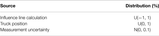
Table 3. Other sources of uncertainty.

The uncertainty from these sources are combined together using Monte Carlo sampling to determine the combined uncertainty PDF. The falsification thresholds for EDMF and the likelihood functions for traditional and modified BMU are determined based on the combined uncertainty PDF using equations (7), (3), and (9), respectively. Equivalent stress ranges at measurement locations obtained using strain gages and the falsification thresholds obtained using equation (7) are shown in Table 4.

TABLE 4

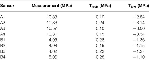
Table 4. Equivalent stress ranges at measurement locations and falsification thresholds for EDMF.

3.5. Structural Identification

In this section, the updated distribution of model parameters obtained using the data-interpretation methodologies is presented.

For residual minimization, samples from the prior distribution of model parameters, E_c and K_deckX are generated through Monte Carlo sampling. For each parameter set, using the surrogate models developed, the equivalent stress range at each sensor location is predicted and the parameter set that provides minimum value for objective function provided in equation (1) is considered as the optimum value.

For EDMF, an initial set of model parameters is generated as a grid. Each model instance is input into the surrogate models developed for equivalent stress range, explained in Section 3.4. Using these surrogate models, the equivalent stress range at each measurement location is obtained and compared with the equivalent stress range obtained using measurement. If the residual between model response and measurement for each location lies within the threshold bounds, T_high,i and T_low,i, computed using equation (7) then the model instance is accepted. All such accepted model instances form the candidate model set, while the remaining model instances are falsified.

In modified and traditional BMU, the posterior PDF is sampled using Markov chain Monte Carlo (MCMC) sampling. The difference between the two Bayesian methodologies is the likelihood function employed. Traditional BMU employs a zero-mean Gaussian likelihood function, as described in equation (3), while modified BMU utilizes a L_∞-norm-based Gaussian likelihood function, as described in equation (9), to update the model parameters.

The candidate model set obtained using EDMF and samples of the joint posterior PDF of primary parameters obtained using modified BMU and traditional BMU are shown in Figure 4.

FIGURE 4

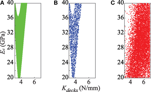
Figure 4. Posterior PDF of primary model parameters as obtained using (A) EDMF, (B) modified BMU, and (C) traditional BMU.

In Figure 4A, each candidate model instance obtained using EDMF is assumed to have an equal probability of occurrence. Figure 4B shows the samples of joint posterior PDF obtained using modified BMU. The sampled region is similar to the candidate model set region obtained using EDMF. This is because of the L_∞-norm-based Gaussian likelihood function used in updating the probability distribution of model parameters. The modified likelihood function has a box-car shape that attributes a constant probability, p, to model instances whose residual when compared to measurements at each sensor location lies within the threshold bounds, T_high,i and T_low,i computed using equation (7). In EDMF, these model instances form the candidate model set. Model instances whose residuals lie outside the threshold bounds for any measurement location are attributed a probability close to zero, which is analogous to falsified model instances in EDMF. Therefore, EDMF and modified BMU provide a similar joint posterior PDF.

Traditional BMU, which assumes a zero-mean Gaussian distribution for the uncertainty associated with the system, provides an informed posterior PDF. The maximum likelihood estimate obtained using traditional BMU for the parameters E_c and K_deckX is 30 GPa and 5.5 log N/mm, respectively. Samples of the joint posterior PDF obtained using traditional BMU is shown in Figure 4C. Using residual minimization, the updated parameter values of E_c and K_deckX obtained are, 20 GPa and 4 log N/mm.

In subsequent sections, the updated model parameters are used to predict the equivalent stress range at two sensor locations and the remaining fatigue life of the bridge at a critical detail. The remaining fatigue life of the bridge is predicted under two scenarios of observed traffic loading, to enable informed decision making regarding intervention for assessment, retrofit, and replacement.

3.6. Equivalent Stress Range Prediction

In this section, the updated model parameters from Section 3.5 are used to predict the equivalent stress range at two sensor locations. The first location is of sensor A5, which is located on the upper flange of the bridge girder as shown in Figure 2. The second location is of sensor B5, which is located on the upper flange of the bridge girder as shown in Figure 2. Measurements from sensors A5 and B5 were not used in model updating. The comparison between equivalent stress range obtained using measurements and predicted using the updated model parameters is shown in Figure 5.

FIGURE 5

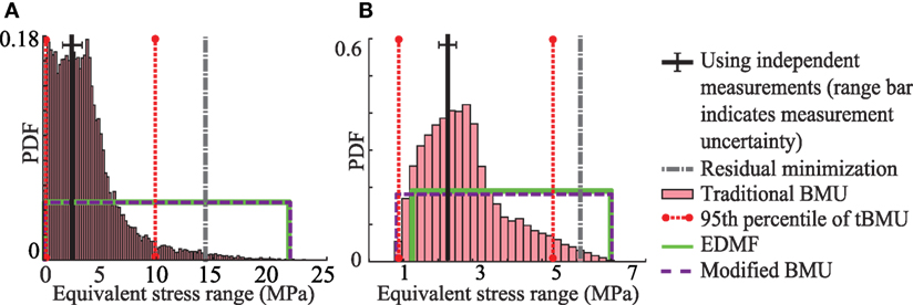
Figure 5. Equivalent stress range predicted using updated model parameters at (A) sensor location A5 and (B) sensor location B5.

In Figure 5A, the equivalent stress range predicted for sensor A5 is shown. The equivalent stress range obtained using strain data from sensor A5 is 2.5 MPa. The equivalent stress range predicted using the prior distribution of model parameters ranges from 0.1 to 24 MPa. Using updated knowledge of bridge behavior as obtained using the three probabilistic data-interpretation methodologies, the prediction range is reduced. Utilizing the updated model parameters obtained using residual minimization, the equivalent stress range predicted is 14.6 MPa, which is biased from the value obtained using measurements. The 95th percentile bounds of equivalent stress range predicted using traditional BMU are 0.1 and 10.1 MPa. Modified BMU and EDMF provide wider and similar bounds ranging from 0.2 to 22 MPa. In this case, all three probabilistic methodologies provide robust prediction of the equivalent stress range at the sensor location as the predicted bounds include the value obtained using measurements.

Figure 5B shows the equivalent stress predicted for sensor B5. The results obtained using the four data-interpretation methodologies again show a similar trend as observed for sensor A5. Residual minimization provides biased prediction of the equivalent stress range at location of sensor B5. The three probabilistic methodologies provide reduced prediction ranges compared with the initial model set prediction. Moreover, the prediction bounds obtained using all three probabilistic methodologies include the equivalent stress range obtained using measurements.

Structural identification for the purpose of damage detection is limited to validation of structural response under uncertainty conditions that are similar to those used for model updating. In this scenario, all three probabilistic methodologies provide robust identification and prediction as shown in Figure 5. In the next section, structural response prediction under uncertainty conditions that are different from that present during identification is presented.

3.7. Remaining Fatigue Life Prediction

Most studies involving structural identification are carried out with the objective of model updating for damage detection. The results obtained are generally validated through prediction as demonstrated in Section 3.6. However, in such a scenario, the uncertainty associated with identification and prediction are similar. Under similar uncertainty conditions all three probabilistic data-interpretation methodologies provide robust predictions, as shown in Figure 5. For the purpose of asset-management decision making, the structural response to be predicted is generally not the response used for identification. Moreover, the loading conditions under which structural response needs to be predicted is likely to be different from those used for identification. Under these conditions, the uncertainties associated with modeling are different during identification and prediction.

In this section, the updated knowledge of bridge response is used to predict the fatigue life of the cover plate detail, which is located close to sensors A1 and A3, shown in Figure 2. The fatigue life prediction is carried out under three loading scenarios. In the first case, the remaining fatigue life of the detail is predicted under the loading duration utilized for identification, from November 18 to 24, 2013 (period 1). In the second case, traffic loading observed during another 1-week period in 2013 (period 2) is utilized for predicting the remaining fatigue life. In the third scenario, traffic loading is simulated for a week assuming 2% annual increase in traffic weight over the next 20 years. The relative combined uncertainty associated with identification of model parameters and prediction of remaining fatigue life is shown in Figure 6.

FIGURE 6

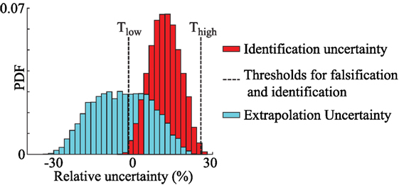
Figure 6. Comparison between identification and prediction uncertainty. In traditional BMU, the bias in uncertainty is assumed to be zero.

The identification uncertainty, shown in Figure 6, is obtained through combination of uncertainty sources specified in Tables 2 and 3. The prediction uncertainty, shown in Figure 6, is obtained through a combination of all modeling uncertainty sources specified in Table 5.

TABLE 5

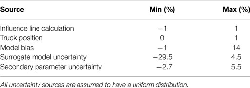
Table 5. Sources of relative prediction uncertainty.

Model bias and surrogate modeling uncertainty are different for identification and prediction. The two primary parameters, E_c and K_deckX, included in the model class for identification are important in developing the surrogate model for equivalent stress range and remaining fatigue life. However, their relationship to the structural responses is different as equivalent stress range and remaining fatigue life are inversely related to each other. The surrogate model developed using neural networks for remaining fatigue life is biased. Along with the model bias, this leads to a biased combined uncertainty PDF for prediction. This difference is taken into account by adding the prediction uncertainty to the remaining fatigue life predicted using the surrogate models.

The Venoge bridge built in 1995 was designed for a service life of 100 years (Eurocode, 1990). As the assessment here is based on traffic data from 2013, the remaining fatigue life of the bridge based on design values is 82 years in 2013. The remaining fatigue life of the bridge predicted using the updated model parameters for traffic loading during period 1 and 2 are shown in Figures 7A,B, respectively.

FIGURE 7

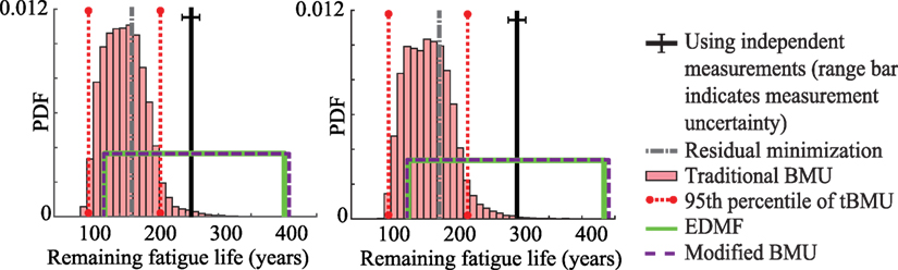
Figure 7. Remaining fatigue life predicted using updated model parameters obtained using the four data-interpretation methodologies for traffic during (A) period 1 and (B) period 2.

In Figure 7, the remaining fatigue life predicted using updated model parameters obtained through the three probabilistic methodologies and residual minimization is shown. These results are compared with the remaining fatigue life obtained using strain measurements from sensor A1. In Figures 7A,B, the remaining fatigue life predicted under traffic loading from period 1 and period 2, are shown, respectively. The prediction uncertainty associated with each case is different as new surrogate models are developed for the respective traffic load duration.

In Figure 7A, the remaining fatigue life obtained using measurements from period 1 is 261 years, while the minimum remaining fatigue life predicted using the prior distribution of model parameters is 92 years. The remaining fatigue life predicted using the updated model parameters obtained using residual minimization is 168 years, which is biased from the value obtained through measurements by 36%. Using traditional BMU, the 95th percentile bounds of predicted remaining fatigue life are 101 and 213 years, which does not contain the remaining fatigue life obtained using measurements. Bias between the MLE of the predicted distribution and the value obtained through measurements is 40%. The bounds of predicted remaining fatigue life obtained using EDMF and modified BMU includes the value calculated using measurements. Using EDMF and modified BMU, the minimum remaining fatigue life predicted using updated model parameters is 127 and 126 years, respectively. Therefore, using measurement data, the minimum remaining fatigue life prediction was improved by 54% compared to the expected service life of 82 years in 2013.

In Figure 7B, the remaining fatigue life obtained using measurements from sensor A1 for traffic loading during period 2, is 302 years. The minimum remaining fatigue life predicted using the prior distribution of model parameters is 99 years. The remaining fatigue life predicted using the updated model parameters obtained using residual minimization is 183 years, which is biased from the value obtained through measurements by 39%. The MLE of remaining fatigue life predicted using traditional BMU is biased from the value obtained through measurement by 45%. Moreover, the 95th percentile bounds on prediction obtained using traditional BMU do not include the value obtained using measurements. Using EDMF and modified BMU, the minimum remaining fatigue life predicted using updated model parameters is increased to 136 and 135 years, respectively. Therefore, using measurement data, the minimum remaining fatigue life prediction was improved by 65% compared to the expected service life of 82 years in 2013.

Traditional BMU provides a biased mean value from the value obtained through measurements for both scenarios. Moreover, the 95th percentile bounds obtained in both cases does not include the value obtained through measurement. Even residual minimization provides biased values for both scenarios considered. EDMF and modified BMU provide robust prediction bounds under both traffic loading scenarios. They help improve the minimum remaining fatigue life prediction by 54 and 65% in the two scenarios considered. Also, EDMF and modified BMU provide similar results, an observation previously made in Figures 4 and 5.

The objective of measurement data-interpretation is to predict structural behavior for future loading scenarios to decide on repair, replace, and retrofit actions. Due to recent trends in transportation, it is likely that freight traffic on highways will increase in future. Therefore, a 2% annual increase in weight of vehicles is assumed over a 20-year period to simulate traffic loading for a 1-week period in the year 2033. Using this traffic loading, the remaining fatigue life of the bridge is predicted as shown in Figure 8.

FIGURE 8

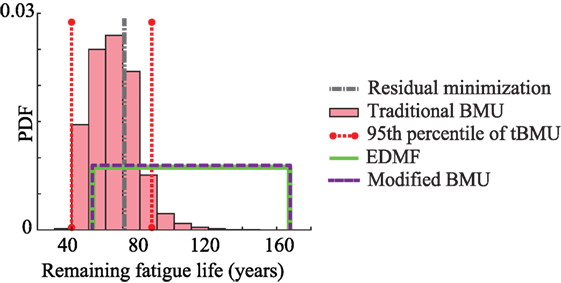
Figure 8. Remaining fatigue life predicted using updated model parameters obtained using the four data-interpretation methodologies for a future traffic loading scenario.

In Figure 8, the minimum remaining fatigue life of the bridge in 2033, predicted using the prior distribution of model parameters is 38 years. The remaining fatigue life predicted using the updated model parameters obtained using residual minimization, traditional BMU (lower 95th percentile bound), EDMF, and modified BMU are 70, 40, 52, and 53 years, respectively. However, as noted in Figure 7, traditional BMU and residual minimization provided biased results from the value obtained using measurements, while EDMF and modified BMU provided robust and accurate bounds. Therefore, the lower bound of remaining fatigue life obtained using EDMF and modified BMU is a robust metric for future decision making. Using measurements, the minimum fatigue life increased from 38 to 52 years, a 37% improvement. Moreover, based on initial design, not accounting for increased loading, the remaining fatigue life of the bridge in 2033 is 62 years, which is greater than the value predicted after model updating. This implies that the bridge if subjected to increased traffic loading will require repair action sooner than expected during initial design, which can be improved through data-interpretation. In the next section, the applicability of these data-interpretation methodologies in practice along with the computation time required will be discussed.

3.8. Applicability in Practice and Computation Time

Application of data-interpretation in practice requires a methodology to satisfy four criteria. First, it should provide accurate identification of model parameters and second, accurate prediction of structural response for reserve capacity estimation. Third, it should be able to incorporate engineering knowledge within the framework. Fourth, the methodology should be easy to understand and use, to enable iterative asset-management decision making.

In Sections 3.5, 6, and 3.7, results obtained using the three probabilistic data-interpretation methodologies and residual minimization are compared. The objective of the comparison in these sections was to elucidate the accuracy of these methodologies to uncertainty conditions in a real environment and the utility of their solutions in practice.

From the perspective of incorporating engineering knowledge into the data-interpretation framework, traditional BMU utilizes a zero-mean Gaussian likelihood function for model updating. Information about model bias is not incorporated in traditional BMU. Moreover, traditional BMU involves the assumption that uncertainty between measurement locations is independent, which is not compatible within a closed system such as civil infrastructure. Residual minimization also cannot include non-parametrized model bias. In traditional BMU and residual minimization, as new sources of uncertainty are identified over the service life of a structure, they can be incorporated into the framework explicitly only as parameters to be identified. Inverse problems such as structural identification have an exponential “O” complexity with respect to number of parameters to be identified. Therefore, increase in the number of parameters to be identified exponentially increases the computation time, which is clearly not desirable.

EDMF and modified BMU provide accurate identification and prediction as shown in Figures 5 and 7. Both methodologies utilize engineering knowledge to determine the combined uncertainty and model bias associated with the system. Then, this information is translated into a falsification criteria for EDMF and into a L_∞-norm-based Gaussian likelihood function for modified BMU. As new information regarding uncertainty sources becomes available, it can be incorporated into the combined uncertainty, thereby not increasing the number of parameters to be identified unless required. This helps in limiting the problem dimension and preventing an exponential increase in computation time. Figure 9 shows the computation time required with increasing number of samples for four combinations of the probabilistic data-interpretation methodologies.

FIGURE 9

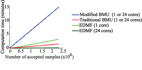
Figure 9. Computation time for identification using four combinations of the probabilistic data-interpretation methodologies. The hardware used for computation is described in Section 3.4.

In Figure 9, comparisons of computation time are provided when the data-interpretation methodologies are utilized in a series and a parallel computation framework. Section 3.4 contains a description of the hardware used in computation. Modified and traditional BMU utilize MCMC sampling to obtain samples of the posterior PDF, while EDMF and residual minimization utilize grid sampling to obtain the updated model parameter values. MCMC sampling is a one-step memory process requiring that samples are generated sequentially. Therefore, MCMC sampling cannot be implemented efficiently in a parallel computation framework. In this case, utilization of multiple cores for computation does not make a significant difference. In grid sampling, samples are generated independently of one another and thus, calculations can be shared more efficiently within parallel configurations, thereby significantly reducing computation time. Other parallel implementations of MCMC sampling are discussed in Section 4.

As shown in Figure 9, modified BMU takes the maximum time to obtain the complete posterior PDF using MCMC sampling. Due to the steep ascent of the box-car-shaped likelihood function before reaching the high-probability plateau, many samples are rejected. To obtain a single accepted sample, many samples are evaluated and rejected. This increases the computation times to obtain the joint posterior PDF. Traditional BMU, which also utilizes MCMC sampling, takes less time than modified BMU as the likelihood function utilized has a gradual slope, which is more favorable for exploring the parameter space. The number of samples rejected before accepting a sample is lower, therefore the total computation time is lower. EDMF takes higher computation time than traditional BMU when grid sampling is utilized. However, once the grid sampling is parallelized with sections of the grid passed to 24 cores for computation, the time taken is reduced. The reduction in computation time is dependent on the number of cores available. In the comparison shown in Figure 9, the parallel computing setup uses 24 cores thereby reducing the computation time for grid sampling by a factor of 24, when computations are completely independent as is the case for grid sampling. Residual minimization, when applied using Monte Carlo sampling, has the same computation time as EDMF using single or multiple cores. A drawback of grid sampling is that, as the number of model parameters increases, the number of parameter combinations to be evaluated increases exponentially. Therefore, optimal model-class selection is very important to limit computational cost without comprising the accuracy of updated model predictions.

The fourth criterion is compatibility of the data-interpretation methodology with knowledge and procedures of practicing engineers. Methodologies should be transparent when updating knowledge of model parameters. MCMC sampling, utilized in traditional and modified BMU, is a black-box algorithm and thus provides low transparency to engineers for understanding the process involved in accepting or rejecting samples. Also, the sampling metrics such as burn-in samples, step size, and number of samples required to obtain a stable solution can be determined only through trial and error. Therefore, many iterations of the sampling process are required to determine these metrics to converge efficiently on to posterior PDFs. EDMF, typically, utilizes grid sampling, wherein a grid of initial model instances is generated. From this initial grid, only model instances whose responses are comparable to measurements within certain bounds of uncertainty (T_high and T_low) are accepted as candidate model instances. The falsification criteria is based on a simple accept-reject decision making. Engineers are able to better understand EDMF, thus increasing robustness of solutions when information changes over service lives of structures.

Currently, residual minimization is the most commonly used methodology. However, as shown in Figures 5 and 7, it does not always provide accurate solutions for estimating reserve capacity. EDMF provides accurate identification and prediction utilizing a simple accept-reject criterion for determining the updated model parameters and requires lower computational resources than other probabilistic methodologies when implemented in a parallel framework.

4. Discussion

Decision making for infrastructure asset management is a complex task, which can be aided through a better understanding of structural behavior using measurements. It is important that the data-interpretation methodology provides accurate predictions while being easy to use and incorporating new information and engineering knowledge over the service life of a structure. Comparison between four data-interpretation methodologies using the Venoge bridge revealed the applicability of these methodologies for reserve capacity estimation. In addition to structural identification (inverse task), the remaining fatigue life of the Venoge bridge (forward task) was predicted under three traffic loading scenarios using updated model parameters. The critical detail analyzed to determine the remaining fatigue life of the bridge is situated in the extended part of the bridge, built in 1995. The design remaining fatigue life of this bridge is 82 years in 2013, which after model updating is estimated to be 126 years.

Residual minimization is a deterministic data-interpretation methodology, which is commonly used in practice due to its ease of understanding. Using updated model parameters obtained through residual minimization, the equivalent stress range at sensors A5 and B5 and remaining fatigue life at a critical detail under two traffic loading scenarios were predicted and compared to results obtained using measurements. The prediction was not accurate in any of the four prediction cases considered. Residual minimization does not always provide robust identification in the presence of unknown correlated uncertainty with model bias and systematic uncertainty, an observation previously noted by Goulet and Smith (2013) for a cantilever beam.

Traditional BMU is a probabilistic methodology that utilizes a zero-mean independent Gaussian likelihood function for model updating. Using updated model parameters obtained through traditional BMU, accurate prediction was observed for only two out of four cases, when compared with results obtained using measurements. Traditional BMU may provide biased predictions when model bias and correlation between uncertainties at measurement locations is not accounted for in model updating. This has been previously observed by Pasquier and Smith (2015) using an idealized simple beam. This paper makes similar observations for a full-scale bridge. Improvement in prediction accuracy may be achieved by parametrizing model bias and correlation between uncertainties at various measurement locations. However, identification of the additional parameters increases dimensionality of the structural identification problem, thereby increasing computational cost and such strategies usually involve assumptions of constant bias at all measurement locations. Also, with few sparse measurements as in the case presented in this paper, a model class with many parameters may lead to unidentifiability (Reuland et al., 2017).

EDMF and modified BMU, which are robust to variations in correlation assumptions, provided accurate identification and prediction for the four prediction cases when compared with results obtained using measurements. Moreover, results obtained using EDMF and modified BMU are similar, implying that EDMF can be understood as an analogous and discrete approach to Bayesian model updating, based on the philosophy of model falsification. This result was previously observed using an idealized simple beam by Pai and Smith (2017). A drawback with application of EDMF for model updating is its sensitivity to presence of outliers in measurements. Therefore, before application of EDMF, it is important to detect outliers in measurement and clean the data.

Predictions obtained using updated model parameters are subject to prediction uncertainty. This prediction uncertainty arises due to the difference between the model used in identification (to predict model response comparable to measurements) and the model used for prediction. In the case studied here, as shown in Figure 6, the identification and prediction uncertainty are different. The prediction uncertainty, similar to identification uncertainty, is computed using engineering knowledge and numerical evaluation of the finite-element and surrogate models. A different prediction uncertainty model, than the one used in this paper, may be employed based on engineering knowledge. However, as prediction results obtained using traditional BMU, modified BMU and EDMF are subjected to the same uncertainty model, the bias between predictions from various methods will not change.

The posterior distribution of model parameters and predictions, such as equivalent stress range and remaining fatigue life, that are obtained through model updating have large uncertainty ranges. The information contained in measurements has not reduced the uncertainty associated with the model parameters significantly. The use of in-service strain and traffic measurements provides engineers with the possibility to gain information without disrupting bridge traffic. However, such measurements are associated with uncertainties such as traffic load position on the bridge, axle weight of the traffic moving on the bridge. Moreover, the strain gages are clustered at two cross-sections of the bridge, thereby the information obtained from these sensors has high redundancy. Better positioning of sensors based on modern measurement system design strategies could help improve the amount of information that is acquired with the sensors. In addition, conducting load tests with knowledge of weight and position of the trucks may help in acquiring additional information. Parameter estimation and prediction can be further refined by improving knowledge of materials through non-destructive testing, improved modeling of the bridge and a more detailed fatigue evaluation with more appropriate S–N curves.

Engineering knowledge of uncertainty sources cannot be included in residual minimization or traditional BMU without increasing the number of parameters to be identified, which increases computation time exponentially. EDMF and modified BMU account for estimation of uncertainty from many sources using engineering knowledge by incorporating it into a combined uncertainty PDF, which is then used to determine either the falsification criteria or the likelihood function. EDMF has an additional advantage as it utilizes a simple accept–reject criterion for model updating, which is easy to understand and implement. Traditional BMU and modified BMU, when applied using MCMC sampling, cannot be implemented efficiently in a parallel computation framework. An alternative may be transitional MCMC sampling proposed by Ching and Chen (2007). Angelikopoulos et al. (2012) have implemented transitional MCMC sampling in a parallel computation framework, wherein independent Markov Chains are generated by individual cores. Usage of transitional MCMC could help in sampling a complex parameter space when the joint posterior distribution of model parameters is multimodal. However, the use of black-box search algorithms decreases the understandability of the methods for use in practice. Comparison of the methodologies is summarized in Table 6.

TABLE 6

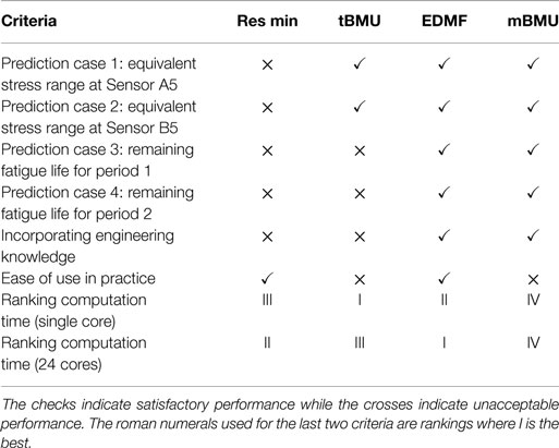
Table 6. Comparison of criteria for the data-interpretation methodologies that are studied in this paper.

As summarized in Table 6, EDMF fulfils all the criteria required of a data-interpretation methodology for use in practice. In addition, grid sampling used in EDMF can be implemented in a parallel computation framework thereby reducing computation cost. EDMF and other data-interpretation methodologies were also used to predict the remaining fatigue life of the Venoge bridge under a future traffic loading scenario. In this scenario, the traffic weight was assumed to increase 2% annually over the next 20 years. The minimum remaining fatigue life predicted after model updating using EDMF, under increased traffic loading, was lower than the service life. Robust prediction of remaining fatigue life for such future scenarios enable use of data-interpretation methodologies in scheduling inspections and deciding on asset-management actions.

5. Conclusion

In this paper, four data-interpretation methodologies are applied to evaluate the fatigue life of a highway bridge under monitored traffic loading. Comparisons are made in terms of parameter identification and accuracy of predictions with respect to measured structural response. Applications of the four methodologies to the Venoge bridge lead to the following conclusions:

• Measurements of service behavior improve the accuracy of remaining fatigue life calculations. The minimum remaining fatigue life of the Venoge bridge is improved by 54% using in-service measurement from eight strain gages and observed traffic load from a WIM station.

• Residual minimization and traditional BMU may not provide accurate predictions in the presence of systematic uncertainty and model bias.

• Modified BMU, which employs a Bayesian framework, explicitly includes model bias and systematic uncertainty in uniform probability distributions and thus provides an accurate prediction of the reserve capacity.

• EDMF provides accurate and similar bounds for remaining fatigue life of the bridge when compared with modified BMU. EDMF has additional advantages compared with Bayesian methodologies due to ease of understanding and compatibility with engineering practice, rejecting unrealistic bridge behavior, while utilizing a simple grid-sampling approach.

• EDMF, when implemented with grid sampling, is an attractive methodology for efficient implementation in a parallel computation framework.

Author Contributions

SP elaborated the application of various data-interpretation methodologies to a full-scale case study for fatigue life evaluation. AN assisted in the elaboration of the case study and fatigue life evaluation. IS was actively involved in developing and adapting the data-interpretation methodologies. All authors reviewed and accepted the final version.

Conflict of Interest Statement

The authors declare that the research was conducted in the absence of any commercial or financial relationships that could be construed as a potential conflict of interest.

Acknowledgments

The authors acknowledge Y. Reuland for fruitful discussions.

Funding

This work was funded by the Swiss National Science Foundation under contract no. 200020-169026 and Singapore-ETH Centre (SEC) under contract no. FI 370074011-370074016.

References

Alvin, K. (1997). Finite element model update via Bayesian estimation and minimization of dynamic residuals. AIAA J. 35, 879–886. doi:10.2514/3.13603

CrossRef Full Text | Google Scholar

Angelikopoulos, P., Papadimitriou, C., and Koumoutsakos, P. (2012). Bayesian uncertainty quantification and propagation in molecular dynamics simulations: a high performance computing framework. J. Chem. Phys. 137, 144103. doi:10.1063/1.4757266

PubMed Abstract | CrossRef Full Text | Google Scholar

Beale, M. H., Hagan, M. T., and Demuth, H. B. (2015). Matlab Neural Network Toolbox User’s Guide Version 8.4. Natick: The MathWorks Inc.

Google Scholar

Beck, J. L. (2010). Bayesian system identification based on probability logic. Struct. Control Health Monit. 17, 825–847. doi:10.1002/stc.424

CrossRef Full Text | Google Scholar

Beck, J. L., and Katafygiotis, L. S. (1998). Updating models and their uncertainties. I: Bayesian statistical framework. J. Eng. Mech. 124, 455–461. doi:10.1061/(ASCE)0733-9399(1998)124:4(455)

CrossRef Full Text | Google Scholar

Behmanesh, I., and Moaveni, B. (2016). Accounting for environmental variability, modeling errors, and parameter estimation uncertainties in structural identification. J. Sound Vib. Elsevier, 374, 92–110. doi:10.1016/j.jsv.2016.03.022

CrossRef Full Text | Google Scholar

Behmanesh, I., Moaveni, B., Lombaert, G., and Papadimitriou, C. (2015). Hierarchical Bayesian model updating for structural identification. Mech. Syst. Signal Process. 64, 360–376. doi:10.1016/j.ymssp.2015.03.026

CrossRef Full Text | Google Scholar

Ben-Haim, Y., and Hemez, F. M. (2012). “Robustness, fidelity and prediction-looseness of models,” in Proceedings of the Royal Society of London A: Mathematical, Physical and Engineering Sciences, Vol. 468 (London: The Royal Society), 227–244.

Google Scholar

Beven, K. J. (2000). Uniqueness of place and process representations in hydrological modelling. Hydrol. Earth Syst. Sci. Discuss. 4, 203–213. doi:10.5194/hess-4-203-2000

CrossRef Full Text | Google Scholar

Brownjohn, J. M. W., De Stefano, A., Xu, Y.-L., Wenzel, H., and Aktan, A. E. (2011). Vibration-based monitoring of civil infrastructure: challenges and successes. J. Civil Struct. Health Monit. 1, 79–95. doi:10.1007/s13349-011-0009-5

CrossRef Full Text | Google Scholar

Brühwiler, E. (2012). Extending the service life of Swiss bridges of cultural value. Proc. Inst. Civil Eng. 165, 235–240. doi:10.1680/ehah.11.00001

CrossRef Full Text | Google Scholar

Brynjarsdóttir, J., and O’Hagan, A. (2014). Learning about physical parameters: the importance of model discrepancy. Inverse Probl. 30, 114007. doi:10.1088/0266-5611/30/11/114007

CrossRef Full Text | Google Scholar

Chang, C.-C., Chang, T., and Xu, Y. (2000). Adaptive neural networks for model updating of structures. Smart Mater. Struct. 9, 59. doi:10.1088/0964-1726/9/1/306

CrossRef Full Text | Google Scholar

Ching, J., and Chen, Y.-C. (2007). Transitional Markov chain Monte Carlo method for Bayesian model updating, model class selection, and model averaging. J. Eng. Mech. 133, 816–832. doi:10.1061/(ASCE)0733-9399(2007)133:7(816)

CrossRef Full Text | Google Scholar

Chou, J.-S., and Pham, A.-D. (2017). Nature-inspired metaheuristic optimization in least squares support vector regression for obtaining bridge scour information. Inf. Sci. 399, 64–80. doi:10.1016/j.ins.2017.02.051

CrossRef Full Text | Google Scholar

Cross, E. J., Worden, K., and Farrar, C. R. (2013). “Structural health monitoring for civil infrastructure,” in Health Assessment of Engineered Structures: Bridges, Buildings and Other Infrastructures, ed. A. Yun (Singapore: World Scientific), 1–31.

Google Scholar

Dowling, N. E. (1971). Fatigue Failure Predictions for Complicated Stress-Strain Histories, Urbana.

Google Scholar

Eurocode. (1990). Basis of Structural Design. 2002. Brussels: European Standard EN.

Google Scholar

Eurocode. (1991). 1: Actions on Structures, Part 2: Traffic Loads on Bridges. Brussels: European Standard EN.

Google Scholar

Farrar, C. R., and Worden, K. (2012). Structural Health Monitoring: A Machine Learning Perspective. Chichester, UK: John Wiley & Sons.

Google Scholar

Frangopol, D. M., and Soliman, M. (2016). Life-cycle of structural systems: recent achievements and future directions. Struct. Infrastruct. Eng. 12, 1–20. doi:10.1080/15732479.2014.999794

CrossRef Full Text | Google Scholar

Friedman, J. H. (1991). Multivariate adaptive regression splines. Ann. Stat. 19, 1–67. doi:10.1214/aos/1176347963

CrossRef Full Text | Google Scholar

Goulet, J.-A., Coutu, S., and Smith, I. F. C. (2013a). Model falsification diagnosis and sensor placement for leak detection in pressurized pipe networks. Adv. Eng. Inform. 27, 261–269. doi:10.1016/j.aei.2013.01.001

CrossRef Full Text | Google Scholar

Goulet, J.-A., Michel, C., and Smith, I. F. C. (2013b). Hybrid probabilities and error-domain structural identification using ambient vibration monitoring. Mech. Syst. Signal Process. 37, 199–212. doi:10.1016/j.ymssp.2012.05.017

CrossRef Full Text | Google Scholar

Goulet, J.-A., Kripakaran, P., and Smith, I. F. C. (2010). Multimodel structural performance monitoring. J. Struct. Eng. 136, 1309–1318. doi:10.1061/(ASCE)ST.1943-541X.0000232

CrossRef Full Text | Google Scholar

Goulet, J. A., and Smith, I. F. C. (2012a). Performance-driven measurement system design for structural identification. J. Comput. Civil Eng. 27, 427–436. doi:10.1061/(ASCE)CP.1943-5487.0000250

CrossRef Full Text | Google Scholar

Goulet, J. A., and Smith, I. F. C. (2012b). Predicting the usefulness of monitoring for identifying the behavior of structures. J. Struct. Eng. 139, 1716–1727. doi:10.1061/(ASCE)ST.1943-541X.0000577

CrossRef Full Text | Google Scholar

Goulet, J.-A., and Smith, I. F. C. (2013). Structural identification with systematic errors and unknown uncertainty dependencies. Comput. Struct. 128, 251–258. doi:10.1016/j.compstruc.2013.07.009

CrossRef Full Text | Google Scholar

Hemez, F., Doebling, S., and Wilson, A. (2002). “Discussion of model calibration and validation for transient dynamics simulation,” in 20th IMAC Conference (Los Angeles, CA).

Google Scholar

Jiang, X., and Mahadevan, S. (2008). Bayesian validation assessment of multivariate computational models. J. Appl. Stat. 35, 49–65. doi:10.1080/02664760701683577

CrossRef Full Text | Google Scholar

Kennedy, M. C., and O’Hagan, A. (2001). Bayesian calibration of computer models. J. R. Stat. Soc. Series B Stat. Methodol. 63, 425–464. doi:10.1111/1467-9868.00294

CrossRef Full Text | Google Scholar

Kuok, S.-C., and Yuen, K.-V. (2016). Investigation of modal identification and modal identifiability of a cable-stayed bridge with Bayesian framework. Smart Struct. Syst. 17, 445–470. doi:10.12989/sss.2016.17.3.445

CrossRef Full Text | Google Scholar

Kwon, K., Frangopol, D. M., and Kim, S. (2010). Fatigue performance assessment and service life prediction of high-speed ship structures based on probabilistic lifetime sea loads. Struct. Infrastruct. Eng. Taylor & Francis, 9, 1–14. doi:10.1080/15732479.2010.524984

CrossRef Full Text | Google Scholar

Li, W., Chen, S., Jiang, Z., Apley, D. W., Lu, Z., and Chen, W. (2016). Integrating Bayesian calibration, bias correction, and machine learning for the 2014 Sandia Verification and Validation Challenge Problem. J. Verif. Valid. Uncertainty Quantification 1, 11004. doi:10.1115/1.4031983

CrossRef Full Text | Google Scholar

Lu, N., Noori, M., and Liu, Y. (2016). Fatigue reliability assessment of welded steel bridge decks under stochastic truck loads via machine learning. J. Bridge Eng. Am. Soc. Civil Eng., 22, 4016105.

Google Scholar

Lynch, J. P., and Loh, K. J. (2006). A summary review of wireless sensors and sensor networks for structural health monitoring. Shock Vibr. Digest 38, 91–130. doi:10.1177/0583102406061499

CrossRef Full Text | Google Scholar

Matsuishi, M., and Endo, T. (1968). Fatigue of metals subjected to varying stress. Jpn. Soc. Mech. Eng. Fukuoka Jpn. 68, 37–40.

Google Scholar

Miner, M. A. (1945). Cumulative damage in fatigue. J. Appl. Mech. 12, A159–A164.

Google Scholar

Moon, F., and Catbas, N. (2013). Structural Identification of Constructed Systems. Reston, Virginia: Structural Identification of Constructed Systems, American Society of Civil Engineers, 1–17.

Google Scholar

Moser, G., Paal, S. G., and Smith, I. F. (2015). Performance comparison of reduced models for leak detection in water distribution networks. Adv. Eng. Inform. 29, 714–726. doi:10.1016/j.aei.2015.07.003

CrossRef Full Text | Google Scholar

Ni, Y. Q., Hua, X. G., Fan, K. Q., and Ko, J. M. (2005). Correlating modal properties with temperature using long-term monitoring data and support vector machine technique. Eng. Struct. 27, 1762–1773. doi:10.1016/j.engstruct.2005.02.020

CrossRef Full Text | Google Scholar

Ni, Y. Q., Zhou, H. F., and Ko, J. M. (2009). Generalization capability of neural network models for temperature-frequency correlation using monitoring data. J. Struct. Eng. 135, 1290–1300. doi:10.1061/(ASCE)ST.1943-541X.0000050

CrossRef Full Text | Google Scholar

Pai, S. G. S., and Smith, I. F. C. (2017). Comparing Three Methodologies for System Identification and Prediction. Cham: Springer International Publishing, 81–95.

Google Scholar

Papadimitriou, C., Beck, J. L., and Katafygiotis, L. S. (2001). Updating robust reliability using structural test data. Probabilist. Eng. Mech. 16, 103–113. doi:10.1016/S0266-8920(00)00012-6

CrossRef Full Text | Google Scholar

Papadopoulou, M., Raphael, B., Smith, I. F. C., and Sekhar, C. (2016). Optimal sensor placement for time-dependent systems: application to wind studies around buildings. J. Comput. Civil Eng. 30, 1–14. doi:10.1061/(ASCE)CP.1943-5487.0000497

CrossRef Full Text | Google Scholar

Pasquier, R., Goulet, J.-A., Acevedo, C., and Smith, I. F. C. (2014). Improving fatigue evaluations of structures using in-service behavior measurement data. J. Bridge Eng. 19, 4014045. doi:10.1061/(ASCE)BE.1943-5592.0000619

CrossRef Full Text | Google Scholar

Pasquier, R., and Smith, I. F. C. (2015). Robust system identification and model predictions in the presence of systematic uncertainty. Adv. Eng. Inform. Elsevier, 29, 1096–1109. doi:10.1016/j.aei.2015.07.007

CrossRef Full Text | Google Scholar

Pasquier, R., and Smith, I. F. C. (2016). Iterative structural identification framework for evaluation of existing structures. Eng. Struct. 106, 179–194. doi:10.1016/j.engstruct.2015.09.039

CrossRef Full Text | Google Scholar

Pasquier, R., D’Angelo, L., Goulet, J.-A., Acevedo, C., Nussbaumer, A., and Smith, I. F. C. (2016). Measurement, data interpretation, and uncertainty propagation for fatigue assessments of structures. J. Bridge Eng. American Society of Civil Engineers, 21, 1–13. doi:10.1061/(ASCE)BE.1943-5592.0000861

CrossRef Full Text | Google Scholar

Popper, K. (1959). The logic of scientific discovery, Hutchinson & Co.

Google Scholar

Reuland, Y., Lestuzzi, P., and Smith, I. F. C. (2017). Data-interpretation methodologies for non-linear earthquake response predictions of damaged structures. Front. Built Environ. 3:43. doi:10.3389/fbuil.2017.00043

CrossRef Full Text | Google Scholar

Rutherford, B. M., Swiler, L. P., Paez, T. L., and Urbina, A. (2006). “Response surface (meat-model) methods and applications,” in Proc. 24th Int. Modal Analysis Conf (St. Louis, MO), 184–197.

Google Scholar

Sanayei, M., Phelps, J. E., Sipple, J. D., Bell, E. S., and Brenner, B. R. (2011). Instrumentation, nondestructive testing, and finite-element model updating for bridge evaluation using strain measurements. J. Bridge Eng. 17, 130–138. doi:10.1061/(ASCE)BE.1943-5592.0000228

CrossRef Full Text | Google Scholar

SIA263/1. (2013). Construction en acier – spécifications compléxmentaires. Zurich: Swiss Society of Engineers and Architects (SIA).

Google Scholar

Šidák, Z. (1967). Rectangular confidence regions for the means of multivariate normal distributions. J. Am. Stat. Assoc. 62, 626–633. doi:10.2307/2283989

CrossRef Full Text | Google Scholar

Simoen, E., Papadimitriou, C., and Lombaert, G. (2013). On prediction error correlation in Bayesian model updating. J. Sound Vibr. 332, 4136–4152. doi:10.1016/j.jsv.2013.03.019

CrossRef Full Text | Google Scholar

Simoen, E., Roeck, G. D., and Lombaert, G. (2015). Dealing with uncertainty in model updating for damage assessment: a review. Mech. Syst. Signal Process. 56–57, 123–149. doi:10.1016/j.ymssp.2014.11.001

CrossRef Full Text | Google Scholar

Simpson, T. W., Mauery, T. M., Korte, J. J., and Mistree, F. (2001). Kriging models for global approximation in simulation-based multidisciplinary design optimization. AIAA J. 39, 2233–2241. doi:10.2514/2.1234

CrossRef Full Text | Google Scholar

Smith, I. F. C. (2016). Studies of sensor-data interpretation for asset management of the built environment. Front. Built Environ. 2:8. doi:10.3389/fbuil.2016.00008

CrossRef Full Text | Google Scholar

Taylor, S. G., Raby, E. Y., Farinholt, K. M., Park, G., and Todd, M. D. (2016). Active-sensing platform for structural health monitoring: development and deployment. Struct. Health Monit. 15, 413–422. doi:10.1177/1475921716642171

CrossRef Full Text | Google Scholar

Vernay, D. G., Raphael, B., and Smith, I. F. C. (2015). A model-based data-interpretation framework for improving wind predictions around buildings. J. Wind Eng. Ind. Aerod. 145, 219–228. doi:10.1016/j.jweia.2015.06.016

CrossRef Full Text | Google Scholar

Worden, K., and Cross, E. J. (2018). On switching response surface models, with applications to the structural health monitoring of bridges. Mech. Syst. Signal Process. 98, 139–156. doi:10.1016/j.ymssp.2017.04.022

CrossRef Full Text | Google Scholar

Worden, K., Farrar, C. R., Manson, G., and Park, G. (2007). “The fundamental axioms of structural health monitoring,” in Proceedings of the Royal Society of London A: Mathematical, Physical and Engineering Sciences, Vol. 463 (London: The Royal Society), 1639–1664.

Google Scholar

World Economic Forum. (2014). Strategic Infrastructure, Steps to Operate and Maintain Infrastructure Efficiently and Effectively, Geneva.

Google Scholar

Yan, W.-J., and Katafygiotis, L. S. (2015). A novel Bayesian approach for structural model updating utilizing statistical modal information from multiple setups. Struct. Saf. 52(Part B), 260–271. doi:10.1016/j.strusafe.2014.06.004

CrossRef Full Text | Google Scholar