Effects of Freestream Turbulence on the Pressure Acting on a Low-Rise Building Roof in the Separated Flow Region

Introduction

In the context of quantifying wind loads on low-rise structures, it has been understood from the time of Jensen (1958) that the mechanical turbulence generated by upwind terrain directly influences the magnitude and spatial distribution of peak pressures of surface-mounted prisms. Numerous studies have shown that accurately simulating freestream turbulence is a necessary condition to achieving dynamic similitude in the boundary layer wind tunnel (BLWT), particularly for characterizing pressure extrema in separated flow regions (e.g., Tieleman et al., 1978; Hillier and Cherry, 1981; Gartshore, 1984; Tieleman, 1992; St Pierre et al., 2005).

Upwind terrain parameters such as the roughness length (z₀) and the displacement height (z_d) are often insufficient predictors of pressure in the so-called “bubble.” The small-scale turbulence must be characterized to evaluate the roll up of the separated shear layer, the reattachment length, and the strength of the vortices advecting through this region (Melbourne, 1979; Kiya and Sasaki, 1983; Tieleman, 1993). The bubble’s average extent, i.e., the mean reattachment length (X_R), is also sensitive to the aspect ratio of the building. For example, composite analysis of multiple BLWT studies by Akon and Kopp (2016) have shown that the mean reattachment length monotonically decreases from smooth terrain to nominally open exposure conditions, plateauing as the surface roughness increases.

These findings—along with recent work to characterize separating shear layers around bluff bodies, e.g., Lander et al. (2017)—continue to shape our understanding of the physical processes that cause extreme pressures to act on the building surface. However, given that a universal approach to predict those pressures remains elusive, there is a strong need for a more comprehensive understanding of the relationship between freestream turbulence and the mechanisms in the shear layer region that govern flow around the body. Therefore, the current study introduces into the public domain a new testbed to complement the limited experiments in this area (e.g., Fang and Sill, 1995; Saathoff and Melbourne, 1997). The study building is the Texas Tech University Wind Engineering Research Field Laboratory (WERFL; Levitan and Mehta, 1992a,b).

Boundary layer wind tunnel results from 33 unique terrains, three geometric scales (1:20, 1:30, and 1:50), and three angles of attack (parallel/perpendicular to the ridgeline and cornering) comprise the data set, which consists of nearly 300 different configurations. Here, we apply the 1:20 model data only. A significant feature of these tests is that the model is, for practical purposes, immersed in all conceivable terrains, ranging from the full inertial sublayer for the smoothest upwind case to the roughness sublayer for the most built-up conditions. The use of two element configurations in the development section also introduces a variation in the displacement height, a scarcely studied subject in wind tunnel modeling of low-rise buildings.

This paper presents comparative results of mean, SD, and peak surface pressures for a subset of the data, and provides new insight on how the pressure loading in separated flow regions changes as a function of higher order moments and the longitudinal turbulence intensity at the eave height of the building. The results show that the spatial distribution of the peaks is heavily influenced by X_R, confirming the functional relationship described in Akon and Kopp (2016). Further, we show that extreme suction under the separation “bubble” collapse if data are normalized by the mean reattachment length and the gust velocity pressure computed from a non-Gaussian peak factor estimator that accounts for the longitudinal turbulence intensity at eave height.

Experimental Design

Experiments were conducted at the University of Florida Natural Hazard Engineering Research Infrastructure Experimental Facility. The BLWT is a low-speed open circuit tunnel with dimensions of 6 m W × 3 m H × 38 m L (Figure 1). Simulation of terrain roughness is performed via the Terraformer, an automated roughness element grid that rapidly reconfigures the height and orientation of 1,116 roughness elements in a 62 × 18 grid to achieve desired upwind terrain conditions 18.3 m along the length of the tunnel. Element dimensions are 5 cm by 10 cm, and they are spaced 30 cm apart in a staggered pattern. Height and orientation can be varied from 0–160 mm and 0–360, respectively. The approach flow was varied by changing the configuration of the Terraformer upwind of the model. Wide and narrow edge windward element orientations were applied. Roughness elements were elevated from 0–160 mm using increments of 10 mm, thus generating 16 upwind terrain conditions for each element orientation—for a total of 33 terrains including the base floor case. The maximum blockage ratio in the tunnel was less than 0.8%.

FIGURE 1

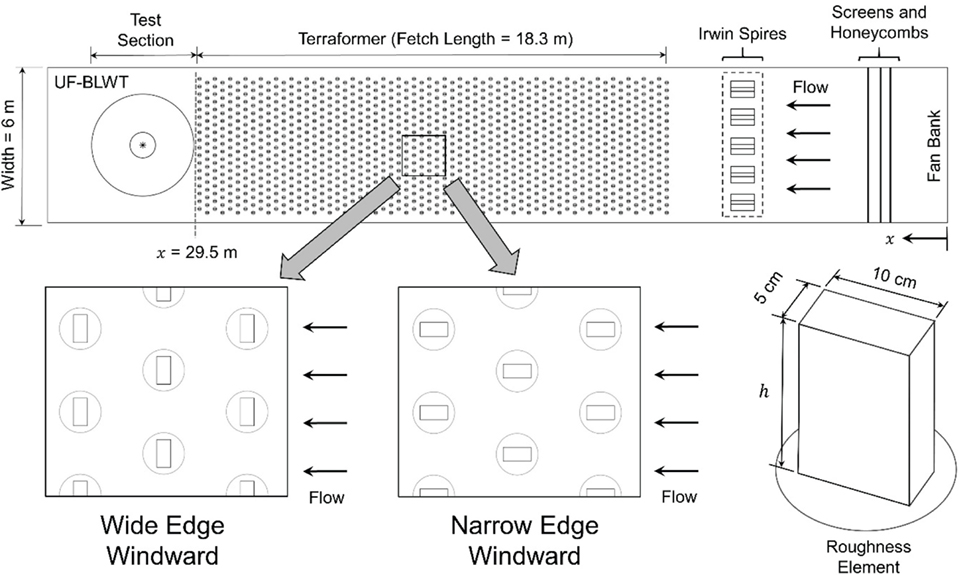
Figure 1. Plan view of the boundary layer wind tunnel (BLWT) at the University of Florida, illustrating the two element orientations considered for this study, namely wide, and narrow edge windward. (Reprinted from Fernández-Cabán and Masters, 2017 with permission from Elsevier).

Approach Flow Conditions

An automated gantry system traversed four Turbulent Flow Instrumentation Cobra pressure probes from across the tunnel for each of the 33 terrain configurations. The probes measure u, v, and w velocity components and static pressure within a ±45° acceptance cone. Response characteristics include a maximum frequency response of 2 kHz and a 2–100 m/s sensing range. Probe accuracy is ±0.5 m/s for standard BLWT operating conditions up to turbulence intensities on the order of 30%. Three vertical traverses were taken at three lateral positions—at the centerline and ±500 mm off the centerline of the tunnel—for each element height increment and element orientations. The triple rotation procedure described in Foken and Napo (2008) was performed to align the probe coordinate system into the streamlines and toward the mean flow coordinate system. Velocity was measured for 60 s at a sampling rate of 1,250 Hz.

Figures 2 and 3 show streamwise mean velocity and turbulence intensity (I_u) profiles for a narrow and wide edge windward element orientation, respectively. Mean velocities are normalized by the reference wind velocity U_ref, at a height of z_ref = 1,670 mm, which was on average 15.3 m/s for all terrain configurations. The elevation was normalized by the eave height of the model (H = 198 mm). The I_u profiles show that a greater range of turbulence levels is generated by orienting the roughness elements in a wide edge windward manner. For instance, I_u exceeds 30% below z/H = 1.5 for an element height of 160 mm for wide edge (Figure 3B). In comparison, maximum turbulence levels for the narrow case are around 21% at elevations below z/H = 1.0. At the eave height of the model, the wide edge element orientation produces I_u = 9–30%, while the narrow case generated turbulence levels ranging from 9 to 21%. Reynolds numbers at eave height (Re = HU_H/v) ranged from 7.8 × 10⁴ (U_H = 6 m/s) for the roughest upwind case (i.e., h = 160 mm, wide) to 14.9 × 10⁴ (U_H = 11.4 m/s) for the flush element configuration.

FIGURE 2

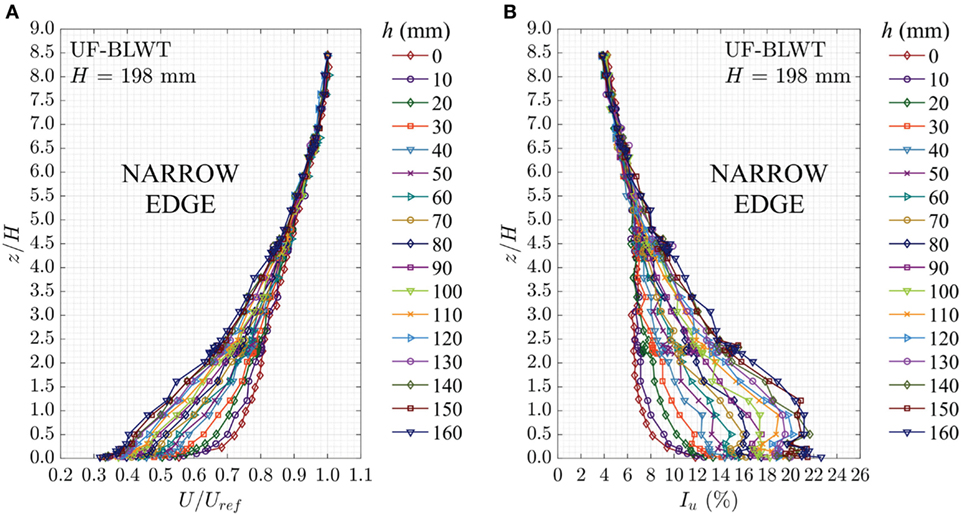
Figure 2. Longitudinal mean velocity (A) and longitudinal turbulence intensity (B) profiles for a narrow edge windward element orientation.

FIGURE 3

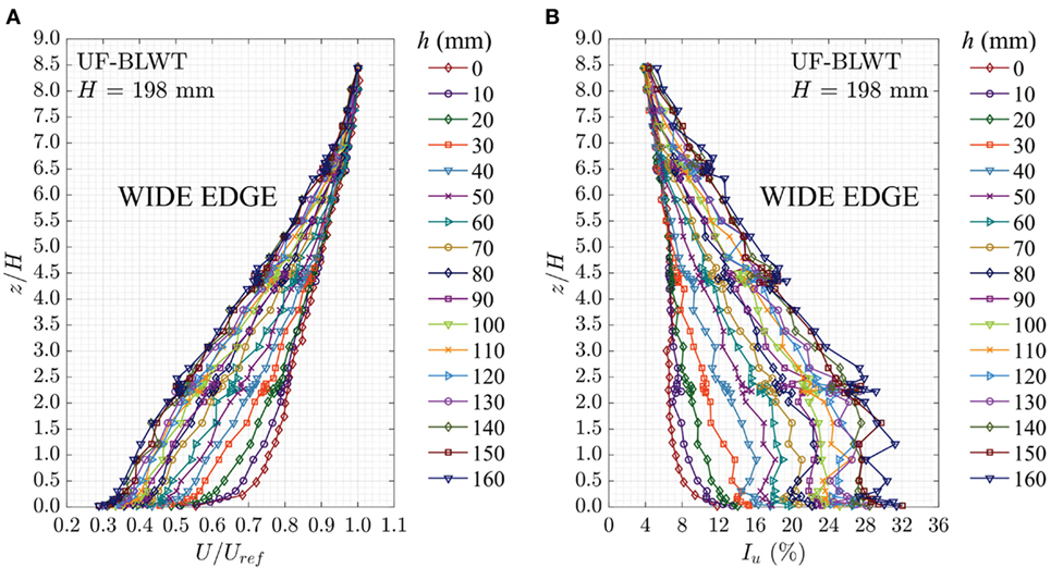
Figure 3. Longitudinal mean velocity (A) and longitudinal turbulence intensity (B) profiles for a wide edge windward element orientation.

Table 1 summarizes estimated aerodynamic and turbulence parameters values at eave height for the full range of element heights and orientations. Turbulence parameters were obtained from probe measurements taken at the eave height of model (z = H). Equivalent full-scale aerodynamic roughness length estimates were obtained from the logarithmic velocity profile:

$z_0=\left(z-z_d\right)\text{exp}\left[-\frac{U_z\mathrm{\kappa }}{u_{\ast }}\right]$ (1)

where u_* is the shear (friction) velocity and κ is the von Kármán constant (~0.4). The zero-plane displacement height was taken as 13.1% of the roughness element height h, following the procedure in Macdonald et al. (1998) that was applied in Fernández-Cabán and Masters (2017). Shear velocities were generated by directly calculating the Reynolds stress from the fluctuating u and w velocity components—i.e., $u_{\ast }^2=\overline{u\prime w\prime }$. The ratio of SD to shear velocity (σ_u/u_*) was fairly constant in the inertial sublayer, with values ranging from 2.0 to 2.1 for all roughness element configurations. These ratios are marginally lower than σ_u/u_* = 2.5 described in ASCE/SEI 49-12 (2012). This difference in σ_u/u_* might be attributed to the lack of large-scale “inactive motion” in the boundary layer (Raupach et al., 1986). Nevertheless, the structure of the separation bubble is mostly dependent on the small-scale turbulent characteristics of the freestream near separated flow regions (Hillier and Cherry, 1981).

TABLE 1

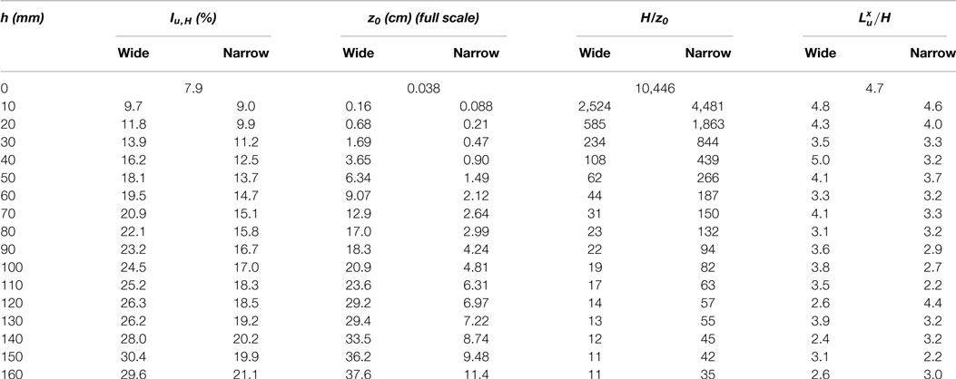
Table 1. Approach flow parameters for the wide and narrow edge windward element orientations.

Longitudinal turbulence spectra at eave height (z = H) for six representative roughness configurations are shown in Figure 4. The spectra are presented in the dimensionless form nS_uu(n,H)/U² and nH/U after Irwin (1998) and Richards et al. (2007). The Von Kármán (1948) spectrum found in ESDU 83045 (1983) was fitted to the measured spectra using equivalent full-scale z₀ values from Table 1, and the measured integral length scales $L_u^x$—obtained from integration of the autocorrelation function. In general, measured $L_u^x$ are at least three times the eave height of the model which is in accordance with minimum requirements in ASCE/SEI 49-12 (2012).

FIGURE 4

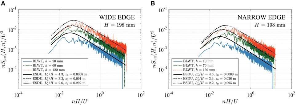
Figure 4. Longitudinal turbulence spectra at a z = 19.8 cm (z = 3.96 m full scale, 1:20 simulation) for a wide (A) and narrow (B) edge element orientations.

Building Model Surface Pressure Measurements

Pressure measurements presented in this study were conducted on the 1:20 rigid building model of the WERFL building. The model was instrumented with 266 pressure taps on the four walls and roof. The tap location follows the same layout as building model “st3” in the NIST aerodynamic database (Ho et al., 2003; see Figure 5), however, 60 additional pressure taps were added on the roof of the model to improve the spatial resolution along tap lines parallel to the long and short building dimension. The model was aligned at 0 and 90 in the approach flow (Figure 6).

FIGURE 5

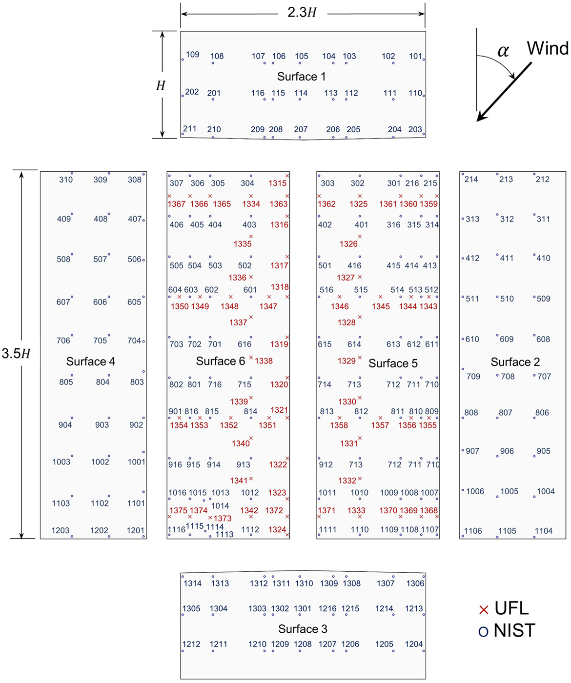
Figure 5. Tap layout for the 1:20 Wind Engineering Research Field Laboratory model. Tap location is identical to building model “st3” in the NIST aerodynamic database (Ho et al., 2003) with the exception of the additional taps indicated by the “X” marker.

FIGURE 6

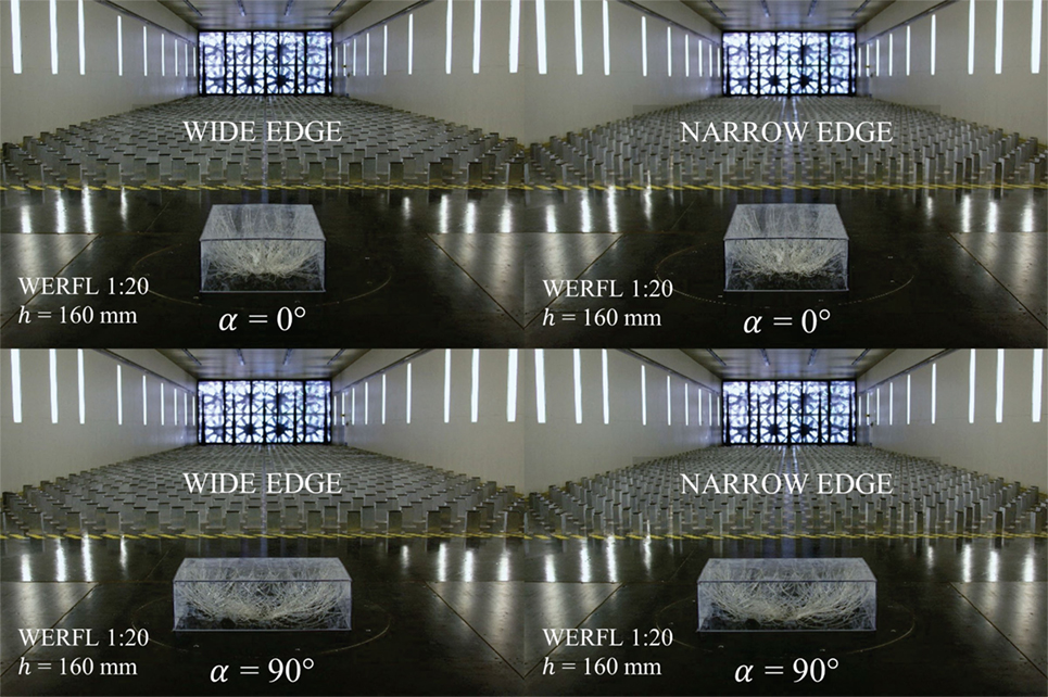
Figure 6. Boundary layer wind tunnel modeling of the 1:20 Wind Engineering Research Field Laboratory (WERFL) building for the narrow and wide roughness element arrangements and the two building orientations considered in this study.

Time series of differential pressures were measured using eight high-speed electronic pressure scanning modules (ZOC33, 2016) from Scanivalve. Urethane tubing cut to a length of 122 cm connected the taps to the pressure scanner. Resonance and damping effects in the tubing system (Irwin et al., 1979) were digitally filtered out using tubing system transfer functions following the approach described in Pemberton (2010). Each experiment was conducted for 300 s at a sampling rate of 625 Hz. Pressure data presented in this work were low-pass filtered 300 Hz to ensure inclusion of significant flow characteristics in the separation bubble—e.g., pseudo-periodic shedding of vortices (Saathoff and Melbourne, 1997). However, cutoff frequencies of 150 and 300 Hz were applied to the complete dataset. Peak pressures that were low-pass filtered at 300 Hz were 5–7% higher than the 150 Hz cutoff frequency.

Unless noted otherwise, external pressure coefficients shown in this paper are calculated as the ratio of the differential pressure and the mean velocity (dynamic) pressure at model eave height:

$C_p\left(t\right)=\frac{P\left(t\right)-P_0}{{\overline{q}}_H}$ (2)

where P(t) is the (absolute) pressure measured, P₀ is the reference (static) pressure, ${\overline{q}}_H=1∕2\rho U_H^2$, ρ is the air density, and U_H is the mean streamwise velocity at eave height estimated from the mean reference velocity pressure in the freestream (U_ref). The reference pressure was converted to the eave height of the building model using an empirical adjustment factor (K) obtained when the model was removed from the turntable:

$U_H=K{U}_{\text{ref}}$ (3)

Static reference pressures (P₀) were taken from the static port of the Pitot tube, ensuring stable measurements with negligible fluctuations. Air density (ρ) was calculated from the air temperature, barometric pressure, and relative humidity measured during each test.

Results

Spatial Distribution of Surface Pressures

Contour subplots of mean pressures (C_p,_mean) measured on the model with the flow streamwise parallel to the long building dimension (α = 0°), are shown in Figure 7. The effect of the freestream turbulence is evident in all cases. Flow over smoother terrains (e.g., h = 10 mm) cause larger reattachment lengths at the leading edge of the structure. As the longitudinal turbulence intensity increases, the mixing in the shear layers increases the rate of entrainment, which decreases the shear layer’s radius of curvature (Gartshore, 1973).

FIGURE 7

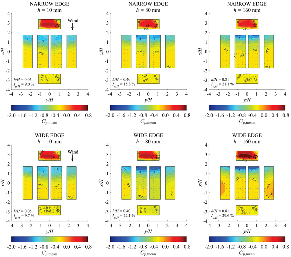
Figure 7. Contours of mean pressure coefficients referenced to the mean velocity pressure at the eave height of the 1:20 model of the Wind Engineering Research Field Laboratory Building.

Standard deviation contour maps of pressure coefficients (C_p,std) are displayed in Figure 8. Differences in the spatial distribution of C_p,std are apparent when comparing the three turbulence levels presented. The largest C_p,std occur near the two corners of the leading edge of the roof for all terrain configurations. However, along the centerline of the roof (y/H = 0), the maximum pressure fluctuations develop closer to the leading edge as the streamwise turbulence increases. For instance, for the roughest case of h = 160 mm (wide edge), C_p,std ~0.8 close to the leading edge, then fluctuations of pressure rapidly decay and stabilize to ~0.3 at approximately x/H = 0.5. In contrast, for h = 10 mm (wide edge), smaller peak values (~0.25 at x/H ~ 1.0) and a more gradual decay of C_p,std is observed (i.e., more spacing between contour lines) along the roof’s centerline. This systematic trend also prevails for the narrow element orientation.

FIGURE 8

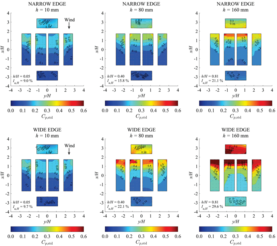
Figure 8. Contours of the pressure coefficient SD referenced to the mean velocity pressure at the eave height of the 1:20 model of the Wind Engineering Research Field Laboratory Building.

Transects of Pressure Along the Roof

The following results describe the surface pressures along designated tap lines shown in Figure 9, which depicts two pairs of densely tapped line transects oriented parallel and perpendicular to the long building dimension, i.e., tap line 1 (TL1), TL2, TL3, and TL4. Tap line pairs (e.g., TL1 and TL2) are symmetric with respect to the centerline of the model.

FIGURE 9

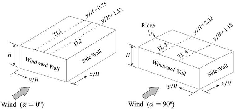
Figure 9. Tap line layout parallel to the long (α = 0^∘) and short (α = 90^∘) building dimensions.

Statistical Measures of the Surface Pressure

Figure 10 displays the distribution of statistical properties along TL1 for 16 terrains (i.e., turbulence levels). The distance from the leading edge is normalized by the eave height of the model (H). The mean pressure is observed to vary by no more than 30% at the leading edge of the structure, with the more turbulent flow causing larger suction. Farther along the roof (x/H > 0.4), this phenomenon reverses as the more turbulent flow reattaches to the roof. The trend in the SD is pronounced, exhibiting nearly a factor of three difference at the leading edge that is on the order of the ratio of the corresponding longitudinal turbulence intensities. Further, the data generally observe the first-order quasi-steady relationship study described in Uematsu and Isyumov (1998), i.e., $C_{p,\text{std}}=2I_u\left|C_{p,\text{mean}}\right|$, which indicates the variations in the approach flow dominate the distortion of the wind around the building with regard to the time varying loads on the structure.

FIGURE 10

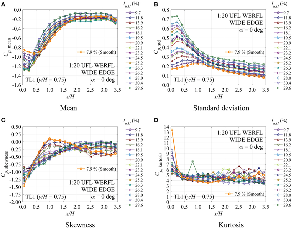
Figure 10. Statistical properties of tap line 1 (TL1) on the 1:20 scale model for the wide edge element case. The distance along the tap line is normalized by the eave height of the model. (A) Mean, (B) SD, (C) skewness, and (D) kurtosis.

The higher order moments (e.g., skewness and kurtosis) exhibit non-Gaussian trends observed near flow separation regions (Holmes, 1981; Sadek and Simiu, 2002). The magnitude of skewness values at the leading edge decreases from -0.8 to -1.4 with increasing turbulence. Kurtosis values rise from ~5 to ~8 close to x/H = 0. Furthermore, in smoother freestream flows (e.g., I_u,H = 9.7%), near Gaussian behavior appears to occur from x/H = 1.0 to 1.5. The roughest upwind cases show close to zero skewness values at x/H > 2.0. However, no clear trend in kurtosis is present in this region.

Reduced Mean Pressure Coefficients

Akon and Kopp (2016) presented a systematic investigation of surface pressures occurring on surface mounted, three-dimensional bluff bodies, finding that the reduced mean pressure coefficient $C_p^{\ast }$ defined in Ruderich and Fernholz (1986):

$C_p^{\ast }=\frac{C_p-C_{p,\text{min}}}{1-C_{p,\text{min}}}$ (4)

produces a suitable match for a broad range geometric scales, building aspect ratios, and terrain conditions. Here C_p refers to the mean pressure coefficient at the location of interest and C_p,min refers to the lowest mean pressure coefficient observed in the tap line under the separation bubble. The application of the Terraformer system enabled characterization of the variation in surface pressure at much finer resolution than previous studies. Figure 11 presents the results for 16 terrains resulting from increasing the element height from 10–160 mm and rotating the elements in the wide (left column) and narrow (right column) orientation to the oncoming flow. In the absence of particle image velocimetry measurements to quantify the distance from the leading edge to the reattachment point (X_R), the empirical relationship developed by Akon and Kopp (2016) (Figure 8) was applied to estimate the value based on the longitudinal turbulence intensity (I_u,H). Tables 2 and 3 list values for the wide and narrow edge element orientations. Tables 2 and 3 show slightly smaller mean reattachment lengths when compared with X_R values presented in Akon and Kopp (2016). The lower X_R values might be a result of the lateral location (y/H) selected for the line transects. In Akon and Kopp (2016), the pressure taps were located along the centerline of the roof surface. Larger mean reattachment lengths should be expected along the roof’s centerline. Conversely, the four tap lines considered in this study were offset from the centerline (Figure 9) of the roof. Therefore, a slight reduction in X_R should be anticipated.

FIGURE 11

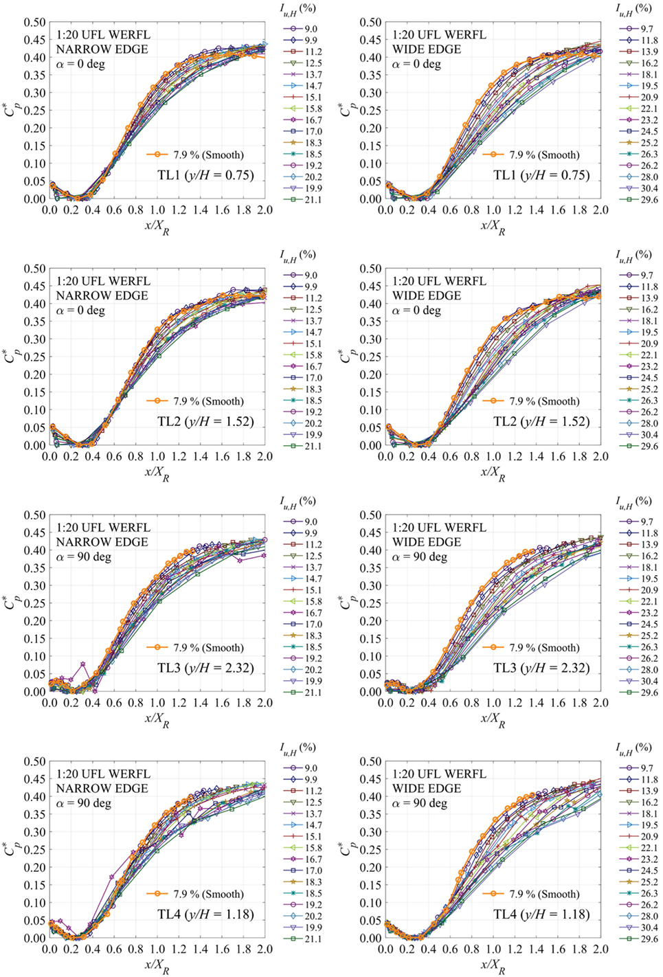
Figure 11. Reduced pressure coefficient transects for the wide and narrow roughness element orientations along tap lines TL1, TL2, TL3, and TL4. The distance from the leading edge is normalized by the mean reattachment length.

TABLE 2

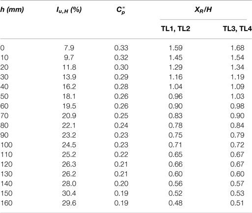
Table 2. Reduced pressure coefficient and mean reattachment length estimates (wide edge).

TABLE 3

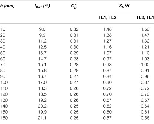
Table 3. Reduced pressure coefficient and mean reattachment length estimates (narrow edge).

A clear pattern appears in all four tap lines. The minimum $C_p^{\ast }$, which corresponds to the worst suction, occurs at x/X_R = 0.3 for every case. In less turbulent flows (i.e., nominally I_u,H < 20%), a reduction in suction at the leading edge is observed (i.e., $C_p^{\ast }$ increases). Above I_u,H = 20% the worst-case suction shifts from x/X_R = 0.3 to x/X_R = 0, indicating a larger suction occurs. Beyond x/X_R = 0.3, the reduced pressure coefficients exhibit a consistent trend. The rougher terrains produce lower $C_p^{\ast }$ in the field of the roof than that of the open exposure, which indicates that the freestream turbulence has a clear effect on the radius of curvature of the shear layer.

Peak Pressure Coefficients

Extreme value analysis was applied to estimate peak surface pressures (Lieblein, 1974) along roof line transects. Figure 12 shows peak pressure coefficients measured along TL1 for wide (Figure 12A) and narrow (Figure 12B) element orientations. Values are computed from a Fisher–Tippett Type I (Gumbel) distribution for a 78% probability of non-exceedance (Cook and Mayne, 1979), and normalized by the mean velocity pressure at eave height as follows:

${Ĉ}_p=\frac{{\widehat{P}}_{78}-P_0}{{\overline{q}}_H}$ (5)

where ${\widehat{P}}_{78}$ is the peak suction of the time history. Figure 12 shows a large spread in peak pressures at the roof’s leading edge with a systematic trend of increasing ${Ĉ}_p$ with freestream turbulence. Turbulence levels for both element orientations show an increase in the magnitude of ${Ĉ}_p$ from approximately -2.5 to -5 for I_u,H = 9.7–21% close to x/H = 0. The higher turbulence intensities produced by the wide edge element orientation results in peak pressures raging from -5 to -9 for I_u,H = 21–29%. Peak pressure curves for both element orientations appear to converge as they progress toward the trailing edge of the roof (x/H = 3.5) where all the peak pressures are approximately unity.

FIGURE 12

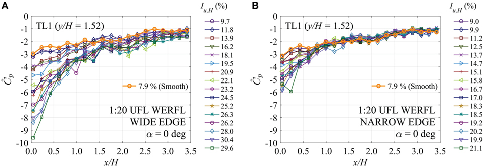
Figure 12. Peak pressure coefficients of tap line 1 (TL1) on the 1:20 scale model for the wide (A) and narrow (B) element orientation. Peak pressures are normalized by the mean velocity pressure at the eave height of the model.

Normalization of Peak Pressure Coefficient Transects

In contrast to the previous section that examined the spatial distribution of pressure minima along the length of the roof, this section evaluates the effect of normalizing the data by the mean reattachment length and the equivalent 3 s gust velocity pressures at full scale, factoring in non-Gaussian behavior. This non-Gaussian trend of the streamwise component has been observed in field experiments and wind tunnel tests (Fernández-Cabán and Masters, 2017). Here, the pressure minima are calculated as:

${Ĉ}_{p,t=3s}=\frac{{\widehat{P}}_{78}-P_0}{{\widehat{q}}_{H,t=3s}}$ (6)

In Eq. 6, ${\widehat{q}}_{H,t=3s}={\overline{q}}_H{\left(\text{GF}\right)}^2$ where GF is the 3 s gust factor computed from the following equation:

$\text{GF}=1+g{I}_{u,H}$ (7)

where g is the 3 s peak factor calculated using a moment-based model presented in Kareem and Zhao (1994) that accounts for the crossing rate, skewness, and kurtosis of streamwise velocity:

$g=\mathrm{\alpha }\left\{\begin{array}{c}\hfill \left(\beta +\frac{\mathrm{\gamma }}{\beta }\right)+h_3\left({\beta }^2+2\gamma -1\right)+\cdots \hfill \\ \hfill h_4\left[{\beta }^3+3\beta \left(\mathrm{\gamma }-1\right)+\frac{3}{\beta }\left(\frac{{\mathrm{\pi }}^2}{12}-\mathrm{\gamma }+\frac{{\mathrm{\gamma }}^2}{2}\right)\right]\hfill \end{array}\right\}$ (8)

where γ is Euler’s constant, 0.5772, $\beta =\sqrt{2\ln \left(\mathrm{\nu }T\right)}$, v is the crossing rate, and T is the duration of the record. The parameters α, h₃, and h₄ are dependent on the third (skewness) and fourth (kurtosis) moments (see Balderrama et al., 2012). Equation 8 is reduced to the well-known peak factor model from Davenport (1964) when the skewness and kurtosis values are set to zero and three, respectively—i.e., Gaussian.

Figure 13 presents peak pressure coefficients for line transect TL1. The distance from the leading edge are normalized by eave height (x/H, left pane) and mean reattachment length (x/X_R, right pane), respectively. It is observed that normalizing the abscissae by X_R shifts the data into horizontal alignment, while normalizing the data by the non-Gaussian velocity pressure causes the data to collapse vertically.

FIGURE 13

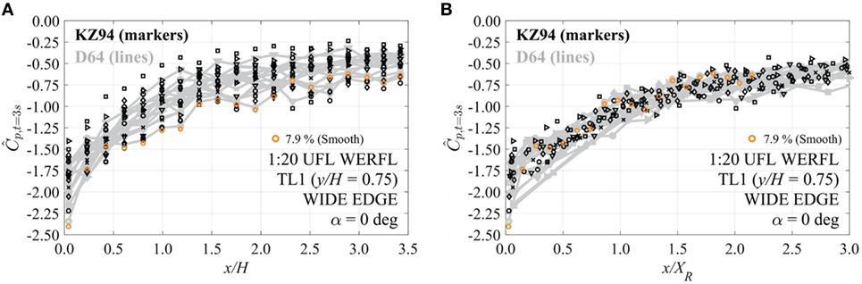
Figure 13. Peak pressure coefficients versus distance from the leading edge normalized by H (A) and X_R (B) along tap line TL1 normal. Peak pressures are normalized by the estimated gust velocity at eave height from Davenport (1964) (denoted by D64) and Kareem and Zhao (1994) (denoted by KZ94) peak factor model.

Tables 4 and 5 contain peak and gust factors at eave height (3.96 m at full scale) for the wide and narrow element orientations, respectively. Peak factors from Davenport (1964) were computed using Eq. 8 and setting the skewness and kurtosis values to zero and three, respectively. This results in g = 3.47 for all element heights and orientations. Thus, it is implied that the peak factor is terrain independent for the Gaussian. In contrast, the non-Gaussian model varies the peak factor from 2.84 to 4.54, which produces a better fit to the data by accounting for increased skewness results in higher peak factors in rougher terrains (I_u,H > 25%) and lower peak factors for smoother exposures (I_u,H ~ 10%) when compared with the Gaussian model (Davenport, 1964).

TABLE 4

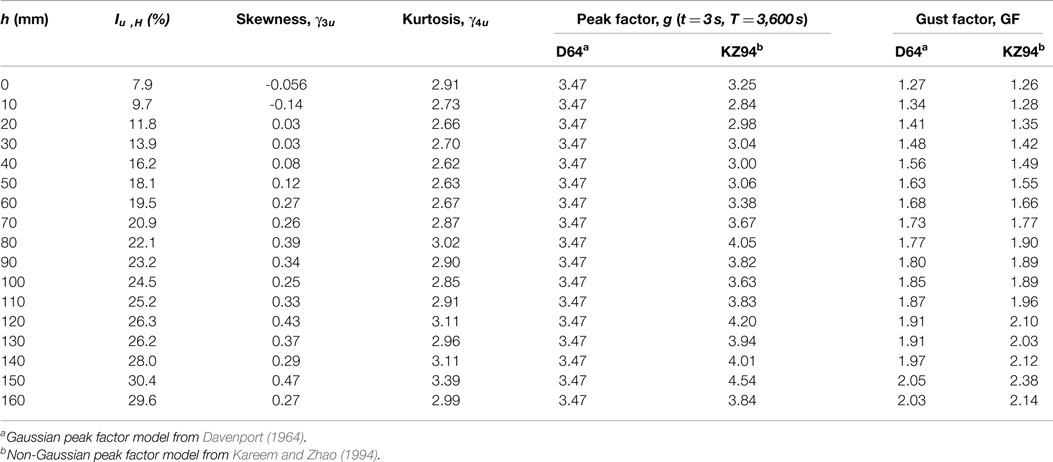
Table 4. Gust factor estimates based on turbulence levels at eave height (wide edge).

TABLE 5

Table 5. Gust factor estimates based on turbulence levels at eave height (narrow edge).

Figure 14 expands the results of Figure 13 to include all tap lines for the narrow and wide edge element orientations. Data fitted to third-degree (i.e., cubic) polynomial curves using a robust linear least-squares fitting method to develop an empirical relation of peak pressures and mean reattachment lengths:

${Ĉ}_{p,t=3s}\left(k=x∕X_R\right)=a_1{k}^3+a_2{k}^2+a_{3}k+a_4$ (9)

where a₁, a₂, a₃, and a₄ are four polynomial coefficients found from the fit. Table 6 includes the corresponding polynomial coefficients, correlation, and root-mean square errors. The results show that the data reasonably collapse for all cases. Little variability is seen in the coefficients and the value at the leading edge (i.e., a₄) are nearly constant for all cases associated with a given wind direction. The effect of the building aspect ratio is evident, however. TL3 and TL4 (associated the with wide side of the building facing windward) produce larger coefficients than TL1 and TL2 due to higher peak pressures near the leading edge caused by the larger flow distortion of the building (see Figure 14).

FIGURE 14

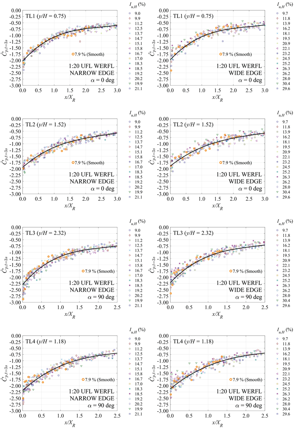
Figure 14. Peak pressure coefficient transects for the narrow (left column) and wide (right column) roughness element orientations normalized by the gust velocity pressure at eave height using a non-Gaussian peak factor model (Kareem and Zhao, 1994).

TABLE 6

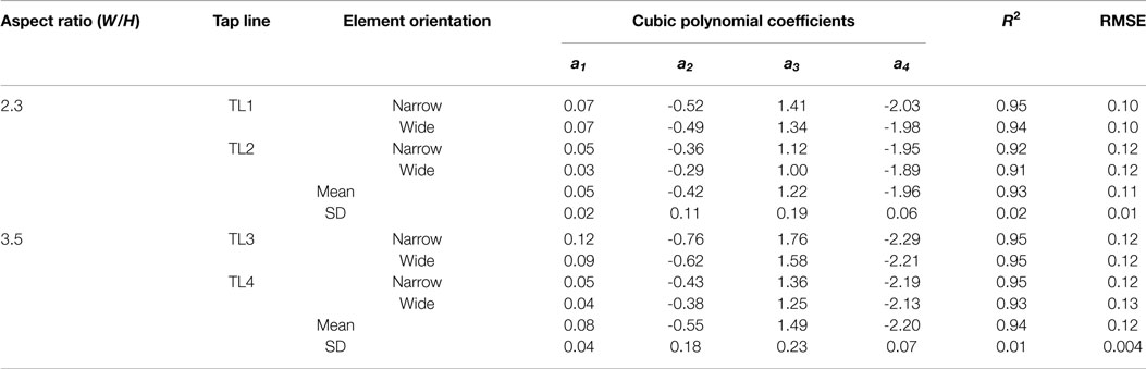
Table 6. Polynomial coefficients from third-order curve fitting of peak pressures as a function of the normalized mean reattachment length.

Normalization of Fluctuating Pressure Coefficients

Analysis was also performed to investigate the effect of such normalization scheme on the distribution of fluctuating roof pressures ($C_p^{\prime }$). Figure 15 includes subplots of normalized SD coefficient ($C_{p,t=3s}^{\prime }$) transects for the narrow and wide roughness element orientations. Similar to Eq. 6, fluctuating pressures are normalized by the 3-s gust velocity pressure (${\widehat{q}}_{H,t=3s}$) at eave height using the non-Gaussian peak factor model (Kareem and Zhao, 1994). Further, the distance from the leading edge is normalized by X_R (contrary to Figure 10B). The family of $C_{p,t=3s}^{\prime }$ transects in Figure 15 appear to collapse when compared with fluctuating pressure distributions shown in Figure 10B. However, the location of maximum $C_{p,t=3s}^{\prime }$ along line transects varies slightly with freestream turbulence. For smoother terrain, the peak $C_{p,t=3s}^{\prime }$ occurs at ~0.6 X_R from the leading edge. Maximum pressure fluctuations for the rougher upstream cases are observed at distances of ~0.35 X_R from the leading edge. These spatial variations of peak $C_{p,t=3s}^{\prime }$ with upstream conditions suggests that normalizing by the non-Gaussian gust velocity pressure might not be sufficient to fully characterize the distribution of pressure fluctuations in the separation bubble, which suggests that the spatial distribution of pressure fluctuations is mainly controlled by the interaction of the approach flow with the structure of the separation bubble and less so by the freestream flow conditions.

FIGURE 15

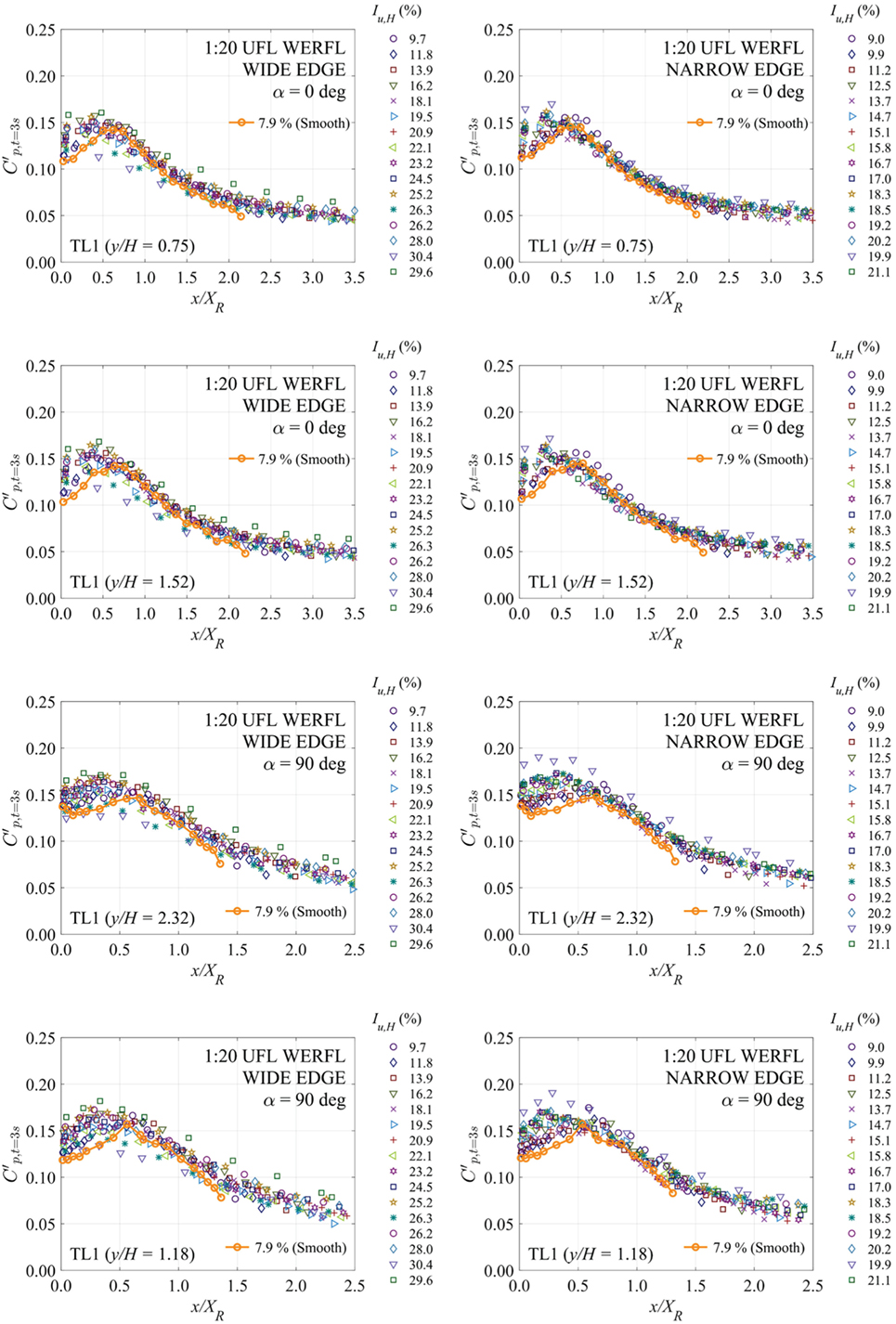
Figure 15. Standard coefficient transects for the narrow (left column) and wide (right column) roughness element orientations normalized by the gust velocity pressure at eave height using a non-Gaussian peak factor model (Kareem and Zhao, 1994).

Discussion

The normalization procedure presented in Section “Normalization of Peak Pressure Coefficient Transects” appears to successfully collapse peak pressures under the separation bubble for a wide range of freestream turbulence levels, with some variation observed at the lead edge of the roof. This collapse of pressure extrema appears to be, in part, attributed to the introduction of non-Gaussian behavior to gust velocity pressure $\left({\widehat{q}}_{H,t=3s}\right)$ estimates—at eave height—used for normalization of surface pressures. However, the normalization scheme was unable to fully collapse fluctuating pressure coefficients within the separation bubble, where the location of maximum pressure fluctuations along the roof tap line varied with freestream turbulence. Thus, the distribution of fluctuating pressures appear to be controlled by the interaction of the turbulent boundary layer with the structure of the separation bubble, while peak pressures can be fully characterized by the freestream flow conditions.

The non-Gaussian peak factor model applied to gust velocity estimates accounts for increased skewness (γ_3u) values observed in the freestream velocity with increasing upwind roughness (or turbulence levels). In rougher terrain, low-rise buildings are partially or entirely immersed in the roughness sublayer (Tieleman, 2003). This layer is not part of inertial sublayer (i.e., “constant” stress region), thus many traditional wind engineering assumptions are no longer valid (e.g., Gaussian behavior). In the roughness sublayer, the flow field is dominated by the presence of non-Gaussian coherent structures (Raupach, 1981; Rotach, 1993). In particular, positively skewed wind fields in the roughness sublayer have been linked to downward motions (i.e., sweep) of high-velocity fluid into the canopy space (Poggi et al., 2004). The increasing trend in skewness of the freestream at eave height with upwind roughness is evident in the present work (Tables 3 and 4). Nevertheless, further research is required to investigate the relation between organized motions in the roughness sublayer and surface pressures on low-rise buildings.

Conclusion and Future Work

A series of BLWT experiments were conducted to investigate the effects of freestream turbulence on low-rise building roofs. A 1:20 model of the WERFL experimental building were immersed in 33 turbulent boundary layer flows via precise regulation of a computer control terrain generator called the Terraformer. The system permitted a fine resolution study of freestream turbulence effects on surface pressures and mean size of separating shear layers around bluff bodies. The paper confirms previous work from Akon and Kopp (2016) concerning the systematic reduction in mean reattachment length with rougher upwind terrains. Furthermore, a standardized form for displaying peak surface pressures close to separating shear layers is presented, where peak pressures are normalized by the gust velocity at eave height and distances along transects are normalized by the mean reattachment length. Gust velocities were computed from a non-Gaussian peak factor model, which appears to collapse the family of peak pressure transects. The normalization scheme is also applied to fluctuating roof pressures. SD coefficient transects corresponding to a family of freestream turbulence levels appear to collapse when normalized by the non-Gaussian gust velocity pressure. However, noticeable variations in the location of maximum pressure fluctuation along line transects are observed for different freestream turbulence intensities. This suggests that the spatial distribution of pressure fluctuations is mostly dominated by the interaction of the turbulent boundary layer with the structure of the separation bubble and less so by the freestream flow conditions.

Subsequent studies will center on further expanding on this work by examining effects of model scale (Stathopoulos and Surry, 1983) and buildings aspect ratio and incorporate more complex upwind terrain conditions (Fang and Sill, 1995) through the generation of random fields of roughness elements to simulate real-world heterogeneous terrain conditions. Further analysis will also be performed on the dataset to closely investigate the coherent (non-Gaussian) flow features in the roughness sublayer and their physical significance to the spatial distribution of surface pressures on low-rise buildings.

Author Contributions

This research builds on the dissertation work of PF (Fernández-Cabán and Masters, 2017), which may be accessed through the University of Florida Library’s Electronic Theses and Dissertations platform (https://cms.uflib.ufl.edu/etd). FM provided valuable guidance in developing the paper in addition to revising the data analysis procedures.

Conflict of Interest Statement

The authors declare that the research was conducted in the absence of any commercial or financial relationships that could be construed as a potential conflict of interest.

Acknowledgments

The authors wish to recognize the Powell Structures and Materials Laboratory staff, with special thanks to Jon Sinnreich, Steve Schein, Eric Agostinelli, Kevin Stultz, and Shelby Brothers for their contribution in wind tunnel testing. Any opinions, findings, and conclusions or recommendations expressed in this paper are those of the authors and do not necessarily reflect the views of the sponsors, partners, and contributors.

Funding

Support for this research was provided by the National Science Foundation CAREER program (CMMI-1055744) with additional support for experimentation through the NSF Natural Hazards Engineering Research Infrastructure (NHERI, CMMI-1520843).

References

Akon, A. F., and Kopp, G. A. (2016). Mean pressure distributions and reattachment lengths for roof-separation bubbles on low-rise buildings. J. Wind Eng. Ind. Aerodyn. 155, 115–125. doi: 10.1016/j.jweia.2016.05.008

CrossRef Full Text | Google Scholar

ASCE/SEI 49-12. (2012). Wind Tunnel Testing for Buildings and Other Structures. Reston, VA: American Society of Civil Engineers.

Google Scholar

Balderrama, J. A., Masters, F. J., and Gurley, K. R. (2012). Peak factor estimation in hurricane surface winds. J. Wind Eng. Ind. Aerodyn. 102, 1–13. doi:10.1016/j.jweia.2011.12.003

CrossRef Full Text | Google Scholar

Cook, N. J., and Mayne, J. R. (1979). A novel working approach to the assessment of wind loads for equivalent static design. J. Wind Eng. Ind. Aerodyn. 4, 149–164. doi:10.1016/0167-6105(79)90043-6

CrossRef Full Text | Google Scholar

Davenport, A. G. (1964). “Note on the distribution of the largest value of a random function with application to gust loading,” in ICE Proceedings, Vol. 28 (London, UK: Thomas Telford), 187–196.

Google Scholar

ESDU 83045. (1983). Strong Winds in the Atmospheric Boundary Layer, Part 2: Discrete Gust Speeds, Engineering Sciences Data Unit. London, UK: Itm. No. 83045.

Google Scholar

Fang, C., and Sill, B. L. (1995). Pressure distribution on a low-rise building model subjected to a family of boundary layers. J. Wind Eng. Ind. Aerodyn. 56, 87–105. doi:10.1016/0167-6105(94)00008-2

CrossRef Full Text | Google Scholar

Fernández-Cabán, P. L., and Masters, F. J. (2017). Near surface wind longitudinal velocity positively skews with increasing aerodynamic roughness length. J. Wind Eng. Ind. Aerodyn. 169, 94–105. doi:10.1016/j.jweia.2017.06.007

CrossRef Full Text | Google Scholar

Foken, T., and Napo, C. J. (2008). Micrometeorology, Vol. 2. Berlin: Springer.

Google Scholar

Gartshore, I. S. (1973). The Effects of Free Stream Turbulence on the Drag of Rectangular Two-Dimensional Prisms. Boundary Layer Wind Tunnel Laboratory, Faculty of Engineering Science, University of Western Ontario.

Google Scholar

Gartshore, I. S. (1984). Some effects of upstream turbulence on the unsteady lift forces imposed on prismatic two dimensional bodies. J. Fluids Eng. 106, 418–424. doi:10.1115/1.3243140

CrossRef Full Text | Google Scholar

Hillier, R., and Cherry, N. J. (1981). The effects of stream turbulence on separation bubbles. J. Wind Eng. Ind. Aerodyn. 8, 49–58. doi:10.1016/0167-6105(81)90007-6

CrossRef Full Text | Google Scholar

Ho, T. C. E., Surry, D., and Morrish, D. P. (2003). NIST/TTU Cooperative Agreement–Windstorm Mitigation Initiative: Wind Tunnel Experiments on Generic Low Buildings. London, ON: The Boundary Layer Wind Tunnel Laboratory, The University of Western Ontario.

Google Scholar

Holmes, J. D. (1981). Non-Gaussian characteristics of wind pressure fluctuations. J. Wind Eng. Ind. Aerodyn. 7, 103–108. doi:10.1016/0167-6105(81)90070-2

CrossRef Full Text | Google Scholar

Irwin, H. P. A. H., Cooper, K. R., and Girard, R. (1979). Correction of distortion effects caused by tubing systems in measurements of fluctuating pressures. J. Wind Eng. Ind. Aerodyn. 5, 93–107. doi:10.1016/0167-6105(79)90026-6

CrossRef Full Text | Google Scholar

Irwin, P. A. (1998). “The role of wind tunnel modelling in the prediction of wind effects on bridges,” in Proceedings of the International Symposium Advances in Bridge Aerodynamics (Copenhagen: Balkema), 99–117.

Google Scholar

Jensen, M. (1958). The model-law for phenomena in natural wind. Ingenioren 2, 121–128.

Google Scholar

Kareem, A., and Zhao, J. (1994). Analysis of non-Gaussian surge response of tension leg platforms under wind loads. J. Offshore Mech. Arct. Eng. 116, 137–144. doi:10.1115/1.2920142

CrossRef Full Text | Google Scholar

Kiya, M., and Sasaki, K. (1983). Structure of large-scale vortices and unsteady reverse flow in the reattaching zone of a turbulent separation bubble. J. Fluid Mech. 154, 463–491. doi:10.1017/S0022112085001628

CrossRef Full Text | Google Scholar

Lander, D. C., Letchford, C. W., Amitay, M., and Kopp, G. A. (2017). Influence of the bluff body shear layers on the wake of a square prism in a turbulent flow. Phys. Rev. Fluids 1, 044406. doi:10.1103/PhysRevFluids.1.044406

CrossRef Full Text | Google Scholar

Levitan, M. L., and Mehta, K. C. (1992a). Texas Tech field experiments for wind loads. Part 1: building and pressure measuring system. J. Wind Eng. Ind. Aerodyn. 43, 1565. doi:10.1016/0167-6105(92)90373-I

CrossRef Full Text | Google Scholar

Levitan, M. L., and Mehta, K. C. (1992b). Texas Tech field experiments for wind loads. Part 1: meteorological instrumentation and terrain parameters. J. Wind Eng. Ind. Aerodyn. 43, 1577. doi:10.1016/0167-6105(92)90373-I

CrossRef Full Text | Google Scholar

Lieblein, J. (1974). Efficient Methods of Extreme-Value Methodology. Technical Report NBSIR 74-602. Washington, DC: National Bureau of Standards.

Google Scholar

Macdonald, R. W., Griffiths, R. F., and Hall, D. J. (1998). An improved method for the estimation of surface roughness of obstacle arrays. Atmos. Environ. 32, 1857–1864. doi:10.1016/S1352-2310(97)00403-2

CrossRef Full Text | Google Scholar

Melbourne, W. H. (1979). “Turbulence effects on maximum surface pressures, a mechanism and possibility of reduction,” in Proc. 5th Int. Conf. on Wind Engineering (Colorado, USA: Pergamon Press), 541–552.

Google Scholar

Pemberton, R. (2010). An Overview of Dynamic Pressure Measurement Considerations. Liberty Lake, WA: Scanivalve Corporation.

Google Scholar

Poggi, D., Porporato, A., Ridolfi, L., Albertson, J. D., and Katul, G. G. (2004). The effect of vegetation density on canopy sub-layer turbulence. Boundary Layer Meteorol. 111, 565–587. doi:10.1023/B:BOUN.0000016576.05621.73

CrossRef Full Text | Google Scholar

Raupach, M. R. (1981). Conditional statistics of Reynolds stress in rough-wall and smooth-wall turbulent boundary layers. J. Fluid Mech. 108, 363–382. doi:10.1017/S0022112081002164

CrossRef Full Text | Google Scholar

Raupach, M. R., Coppin, P. A., and Legg, B. J. (1986). Experiments on scalar dispersion within a model plant canopy part I: the turbulence structure. Boundary Layer Meteorol. 35, 21–52. doi:10.1007/BF00117300

CrossRef Full Text | Google Scholar

Richards, P. J., Hoxey, R. P., Connell, B. D., and Lander, D. P. (2007). Wind-tunnel modelling of the Silsoe Cube. J. Wind Eng. Ind. Aerodyn. 95, 1384–1399. doi:10.1016/j.jweia.2007.02.005

CrossRef Full Text | Google Scholar

Rotach, M. W. (1993). Turbulence close to a rough urban surface part I: Reynolds stress. Boundary Layer Meteorol. 65, 1–28. doi:10.1007/BF00708816

CrossRef Full Text | Google Scholar

Ruderich, R., and Fernholz, H. H. (1986). An experimental investigation of a turbulent shear flow with separation, reverse flow, and reattachment. J. Fluid Mech. 163, 283–322. doi:10.1017/S0022112086002306

CrossRef Full Text | Google Scholar

Saathoff, P. J., and Melbourne, W. H. (1997). Effects of free-stream turbulence on surface pressure fluctuations in a separation bubble. J. Fluid Mech. 337, 1–24. doi:10.1017/S0022112096004594

CrossRef Full Text | Google Scholar

Sadek, F., and Simiu, E. (2002). Peak non-Gaussian wind effects for database-assisted low-rise building design. J. Eng. Mech. 128, 530–539. doi:10.1061/(ASCE)0733-9399(2002)128:5(530)

CrossRef Full Text | Google Scholar

St Pierre, L. S., Kopp, G. A., Surry, D., and Ho, T. C. E. (2005). The UWO contribution to the NIST aerodynamic database for wind loads on low buildings: Part 2. Comparison of data with wind load provisions. J. Wind Eng. Ind. Aerodyn. 93, 31–59. doi:10.1016/j.jweia.2004.07.007

CrossRef Full Text | Google Scholar

Stathopoulos, T., and Surry, D. (1983). Scale effects in wind tunnel testing of low buildings. J. Wind Eng. Ind. Aerodyn. 13, 313–326. doi:10.1016/0167-6105(83)90152-6

CrossRef Full Text | Google Scholar

Tieleman, H. W. (1992). Problems associated with flow modelling procedures for low-rise structures. J. Wind Eng. Ind. Aerodyn. 42, 923–934. doi:10.1016/0167-6105(92)90099-V

CrossRef Full Text | Google Scholar

Tieleman, H. W. (1993). Pressures on surface mounted prisms: the effects of incident turbulence. J. Wind Eng. Ind. Aerodyn. 49, 289–300. doi:10.1016/0167-6105(93)90024-I

CrossRef Full Text | Google Scholar

Tieleman, H. W. (2003). Wind tunnel simulation of wind loading on low-rise structures: a review. J. Wind Eng. Ind. Aerodyn. 91, 1627–1649. doi:10.1016/j.jweia.2003.09.021

CrossRef Full Text | Google Scholar

Tieleman, H. W., Reinhold, T. A., and Marshall, R. D. (1978). On the wind-tunnel simulation of the atmospheric surface layer for the study of wind loads on low-rise buildings. J. Wind Eng. Ind. Aerodyn. 3, 21–38. doi:10.1016/0167-6105(78)90026-0

CrossRef Full Text | Google Scholar

Uematsu, Y., and Isyumov, N. (1998). Peak gust pressures acting on the roof and wall edges of a low-rise building. J. Wind Eng. Ind. Aerodyn. 77–78, 217–231. doi:10.1016/S0167-6105(98)00145-7

CrossRef Full Text | Google Scholar

Von Kármán, T. (1948). Progress in the statistical theory of turbulence. Proc. Natl. Acad. Sci. U.S.A. 34, 530–539. doi:10.1073/pnas.34.11.530

CrossRef Full Text | Google Scholar

ZOC33. (2016). Miniature Pressure Scanner. Available at: http://scanivalve.com/products/pressure-measurement/miniature-analog-pressure-scanners/zoc33-miniature-pressure-scanner/ (Accessed: March 13, 2018).

Google Scholar