The Mediterranean Basin and Southern Europe in a warmer world: what can we learn from the past?

1. Introduction

Over the past two decades, the concepts of climate change and cultural shift have often been coeval in the Mediterranean (deMenocal, 2001; Staubwasser and Weiss, 2006). This connection suggests that mechanisms involved in cultural evolutions over the last 10,000 years may result from adaptive processes and/or inventions in response to the cumulative pressure from societal and environmental forcings. Climate may thus be considered one of the key factors that spawned innovation or that accelerated and magnified social crises throughout history. Previous research has shown that the issue of climate is recurrent in the study of Mediterranean civilizations, with a focus on the potential links between climate pressures, environmental thresholds for agricultural innovations, mass migrations and abandonment of territory (deMenocal, 2001; Weiss, 2001; Staubwasser and Weiss, 2006). In particular, extreme droughts may induce either technological and ideological advances or socio-economic declines that lead to important population movements (Reuveny, 2007). Although the attitude and governance strategies toward drought have changed in industrial societies (Sowers et al., 2011), the socio-economic aftermath of the 2007–2009 drought in the historical region of the Fertile Crescent (Trigo et al., 2010) has clearly compromised the common view that modern agricultural societies, through technological improvement and societal adjustment, adaptively protect themselves from precipitation anomalies (Lobell et al., 2008).

The Mediterranean winter climate is mostly dominated by the westward moving storms that originate over the Atlantic, and by internal cyclonic storms produced by the orography (Lionello et al., 2008). In the Middle East, the mountainous regions of eastern Turkey and northern Iraq vitally induce orographic precipitation that supplies water to the Euphrates and Tigris Rivers, which play a crucial role feeding the Mesopotamia region (Evans et al., 2004). The Mediterranean has historically been a vulnerable region to climatic changes (Giorgi, 2006). Model-based scenarios (Giorgi and Lionello, 2008; Stocker et al., 2013) project a temperature increase between 0.5 and 5°C and a total precipitation decrease between 0 and 30% around the Mediterranean, mainly in the summer. This will aggravate the water deficit in these regions where irrigation and population pressures already strain the water supplies.

Because changes in water availability exert significant pressure on resources in dry environments, ecosystems are critically dependent on soil moisture provided by seasonal rain or spring snowmelt. Opportunistic annual plant species may rapidly grow in response to soil-induced humidity and the vegetation greenness is mainly related to recent precipitation (Zaitchik et al., 2007). But winter crops and persistent vegetation depend on deep soil moisture, and the vegetative cycles are the result of the combined effects of precipitation and evaporation, as well as temperature in mountainous regions (Trigo et al., 2010). The present vegetation is considered as the outcomes of the Mediterranean climate modulated by successive but irregular events of enhanced aridity and increasingly frequent human impacts since the early Neolithic. These may be reconstructed using vegetation and isotopic proxies in lacustrine sediments (Roberts et al., 2011). Pollen-based reconstructions of temperatures during the Holocene have shown relatively lower temperatures in the Mediterranean region than in higher latitudes (Davis et al., 2003); however, isotope-based reconstructions of precipitation have shown a delayed precipitation decrease nearing the present values in the western Mediterranean when compared with the eastern Mediterranean (Roberts et al., 2011). As climate model simulations can reproduce the spatial patterns of climate variables (Brayshaw et al., 2011), the physical consistency of the reconstructions is validated. Furthermore, most of the reconstructions performed at various sites show a high variability in precipitation at the centennial scale (Gasse and Roberts, 2004). All of these results confirm the vulnerability of the Mediterranean climate at various time scales, but the extent of the modern climate change compared with climate change in the Holocene remains uncertain.

To understand the potential consequences of warmer and drier conditions on future vegetation dynamics, human behavior and ecosystem services in the sensitive Mediterranean region, the long-term climate dynamics and the severity of modern vs. historical droughts must be assessed. As deterioration of water supply and rivalry for remaining resources may also be one of the outcomes of the global change, there is moreover a need to characterize if water stresses acted like a “threat multiplier” (Evans, 2009) for the periods when powerful civilizations declined.

Using an inverse modeling method, we reconstructed maps of various climate anomalies by step of 100 years. The climate variables concern winter and summer temperatures, water availability for the vegetation, annual temperature, and precipitation, but we will focus on annual precipitation and temperature. This approach, in the framework of the Bayesian paradigm, is particularly suited for dealing with large dissimilarities between past and present, especially the direct effect of strong CO₂ increase on vegetation photosynthesis.

2. Data and Methods

The climate is reconstruted using a data-model approach (Guiot et al., 2014). The data are pollen combined to the vegetation model BIOME4 (Kaplan et al., 2003). The model calculates primary productivity of vegetation types from climate values. The primary productivities (outputs of the model) are compared to pollen data and we estimate the model inputs, i.e., the climatic values. This has already been applied in paleoclimatology by Guiot et al. (2000); Wu et al. (2007); Guiot et al. (2009); Garreta et al. (2010). Here the originality is that the inversion is done time-slice by time-slice to keep the spatial coherency of the data. So we hope to be coherent with the atmospheric circulation pattern which have constrained the climate of each time-slice.

2.1. Pollen Data

Pollen data have been extracted from the European Pollen Database (http://www.europeanpollendatabase.net) and completed by six cores published by Kaniewski et al. (2013). A set of 286 sites (Figure 1) are available in the [10W, 50E; 30N, 50N] window, representing 16474 spectra from 10 ka BP to now. The northern part of the Mediterranean Basin is clearly dominant, and southwest is only covered by a few sites. The references of the data are given in Appendix 1.

FIGURE 1

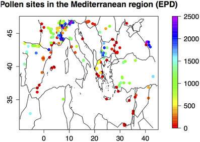
Figure 1. Map of the 295 sites used for the reconstruction; the color indicates the elevation of the site.

Pollen taxa are aggregated into plant pollen types according to the method of Prentice et al. (1996).

2.2. Climatic Data

We used the gridded climatic data at a monthly time-step from 1901 to 2000 provided by the British Atmospheric Data Centre (BADC). For temperature, precipitation and cloud cover, we used the file CRU_TS_3_10 which has a spatial resolution of 0.5° (http://badc.nerc.ac.uk). The gridpoints has been aggregated at a 2° increment for latitude, from 31 to 49°N and 4° incrementfor longitude, from 9°W to 47°E, using the interp.surface() function (interpolation using bilinear weights) of package fields (http://www.image.ucar.edu/Software/Fields). This area contains 95 terrestrial gridpoints. We removed the gripoints which did not have close pollen sites, so the area was restricted to 81 gridpoints. The time-series are averaged on the 1901–2000 period, providing a (81,36)-matrix. A principal component analysis is applied to correlation matrix of this dataset to extract the main information in a few orthogonal variables. The first two PCs explain 76% of the total variance. The first one is negatively correlated with temperatures, mainly April to October, and all monthly sunshine variables in opposition to May to September precipitation; the second is negatively correlated with October to April precipitation. Considering that the PCs are much less correlated with monthly variables (correlation <0.5 in absolute value), we retain these first two variables to represent the spatial variance of the 36 climate monthly variables.

These PC's will be used as a small set of a independent variables from which the three climatic fields (temperature, precipitation, sunshine duration) can be estimated. There is a main reason to this approach: the vegetation model inversion is only possible with a reduced set of parameters. The estimation of monthly temperature, precipitation and cloudiness is done by multiple regression on these three principal components, using the 81 gridpoints as observations. The proportion of explained variance is high and ranges from 0.58 to 0.92. The lowest is found for the cloudiness durations (Figure 2).

FIGURE 2

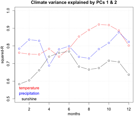
Figure 2. Proportion of the variance explained by the first two principal components in function of the number of the month.

2.3. The CO₂ Atmopsheric Concentration Series

The CO₂ atmospheric data for the last 10,000 years have been taken from the ice core of Taylor Dome in Antarctica (77.78°S, 158.72°E, 2365 m) (Indermühle et al., 1999). The series is composed by 75 values from 11,103 years BP to now. The minimum concentration was found at about 8000 years BP (260 ppmv) and the maximum at about 1980 AD (340 ppmv). The series have been interpolated at an centennial time-step using a spline function (Figure 3).

FIGURE 3

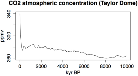
Figure 3. Time-series of CO₂ concentration measured in the Taylor Dome ice core and interpolated at the 100 years time-step. After Indermühle et al. (1999).

2.4. The Vegetation Model BIOME4

There exists a large variety of vegetation models. Some of them need fine information on climate to estimate vegetation. They are hardly usable at a continental scale where the climate information is often restricted to monthly records. This explains why paleostudies have used relatively simple biogeochemical models. A popular model in paleoclimatology is BIOME3 (Haxeltine and Prentice, 1996) or a modified version BIOME4 (Kaplan et al., 2003). It is a process-based terrestrial biosphere model which includes a photosynthesis scheme that simulates acclimation of plants to changed atmospheric CO₂ by optimization of nitrogen allocation to foliage and by accounting for the effects of CO₂ on net assimilation, stomatal conductance, leaf area index (LAI) and ecosystem water balance. It assumes that there is no nitrogen limitation. The inputs of the model are soil texture, CO₂ rate, absolute minimum temperature (T_min, °C), monthly mean temperature (T, °C), monthly total precipitation (P, mm) and monthly mean sunshsine (S, %), i.e., the ratio between the actual number of hours with sunshine over the number of day hours. From these input variables, the model computes bioclimatic variables, and from them, the net primary production (NPP, in kg m⁻²years⁻¹) for the plant functional plants (PFT) able to live in this input climate. Competition among PFT's is simulated by using the optimal NPP of each PFT as an index of competitiveness. The most important PFT's in the Mediterranean Basin are: temperate broadleaved evergreen trees (tbe), temperate summergreen trees (tst), temperate evergreen conifer trees (ctc), boreal evergreen trees (bec), boreal deciduous trees (bs), temperate grass (tg), C4 grass (trg4), woody desert plant type (wd), tundra shrub type (tus), cold herbaceous type (ch). The pollen PFT's are sometimes more precise and pollen information is sufficient to recognize several varieties of the same model-based PFT, for example pollen is able to separate warm and cool ts (Tarasov et al., 1998). The use of such models in the paleoclimatological context and the simulation of the CO₂ effect on ecosystems is reviewed in Prentice and Harrison (2009).

2.5. The Inversion Algorithm

To reconstruct climate from pollen data, it is necessary to implement relationships where pollen assemblages are the inputs and climate is the output. But vegetation models use climate as inputs. The idea proposed by Guiot et al. (2000) for this problem is then to use massive computation algorithms to invert the model, starting from vegetation and going back to climate. It is not an analytical inversion, but an iterative procedure where one converges progressively toward the climate which has produced the observed vegetation. The climatic space is randomly sampled to produce a large variety of climatic scenarios which are introduced in the vegetation model to simulate the corresponding vegetation composition and productivity. The simulated pollen assemblages are compared to the fossil assemblage and those matching reasonably well are retained. The corresponding climatic scenarios are then considered to be compatible with the observed vegetation. They are used to build histograms, which are estimates of probability distribution functions of a climate able to generate such a vegetation. This implies a measure of coherency between outputs of the model and the pollen assemblages (see Section 2.6).

An important point is the number of input climatic parameters. BIOME4 uses 36 monthly climate inputs above described and we consider 81 gridpoints. One has to modify them randomly to browse the climatic space, but its number is too high (36 × 81) to converge. So, we reduce them to a small number of representative variables from which all the other climatic variables are deduced. These are the two PC's of the mean climatic field and we use the regressions explained in Section 2.2 to estimate the 36 climatic variables needed by BIOME4.

Inversion of the model is done under the paradigm of Bayesian theory (Robert and Casella, 2013). It uses the concept of prior and posterior probability distribution. The prior is the information, summarized under the form of a distribution, which is available prior to the data analysis. The posterior is the information that we will deduce from the combination of data and a hierarchical model. In that respect, the hierarchical model is not restricted to the vegetation model, but it is the function which relates the prior to the posterior. In statistical terms, it is the probability of climate C conditional to pollen assemblages. It is noted, according to the Bayes' law:

$\begin{array}{cc}p(C\mid Y)\propto f(Y\mid C)p(C)& \left(1\right)\end{array}$

where p(C) is the prior distribution of climate C and f(Y | C) is the likelihood function of pollen assemblages given the climate (as provided by the model from the climate). The prior is an initial guess of the probability distribution of the climate. It can be given by the knowledge we have from modern climate variability or from, if we work on periods much different from the present one, from the knowledge which has been accumulated in palaeclimatology. The distribution law is then an uniform law defined on the so defined range. Likelihood function is provided by the comparison of BIOME4 model simulations given a large set of climate scenarios to observed pollen assemblages.

Bayesian statistics have been conceptually introduced in paleoclimatology by Korhola et al. (2002) and Haslett et al. (2006), but without any reference to a mechanistic model and by Guiot et al. (2000) with a less rigorous formalism but with a mechanistic model. The first ones underlined that such an approach is slow despite making unreasonable compromises on the models employed. With a mechanistic model, it is even slower. The reason is that, to draw the posterior, one has to use Monte-Carlo algorithms which need thousands of iterations. These algorithms—coherently with the Bayesian inference—provide an integration over the climate parameter space instead of an optimization. A popular type of such algorithms is known as Monte Carlo Markov Chain (MCMC) algorithm. Let us consider a multi-dimensional mathematical space where each dimension represents a climatic variable. A vector of parameters is an element of the multi-dimensional climate space. The Metropolis-Hastings algorithm is an iterative method which browses the climate space according to an acceptance-rejection rule (Metropolis et al., 1953; Hastings, 1970). The output of this algorithm is a path or chain of climate parameters describing the posterior distribution of climate parameter. The MCMC algorithm can be considered as an equilibrium inversion method, compatible with equilibrium vegetation models as BIOME4.

We use the “metrop” function of the R-package “mcmc” (http://www.stat.umn.edu/geyer/mcmc/). This function needs an evaluation of the likelyhood function (Equation 1). As BIOME4 is a very complicated function, we have reduced the problem to a very simple case where the pollen pft vector (data) is equal to the NPP pft vector (model) plus a Gaussian error term of mean 0 and variance σ²I (I being the unit matrix of size m). So we assume that the m pft errors have the same variance and are independent. This can be a strong hypothesis and is only acceptable because the pollen pft scores and the simulated pft's are standardized (here by division by their respective sum). In this case, the log-likelihood function is

$\begin{array}{cc}LH\propto -K-\frac{1}{2{\sigma }^2}{\displaystyle \sum _{i=1}^n{(Y_i-\widehat{Y_i})}^2}& \left(2\right)\end{array}$

Y_i is the observed pollen score of pft i and $\widehat{Y}$_i is the corresponding simulated NPP i. This LH function is a similarity function between data and model.

As both datasets are not available on the same sites, we need some developments before computing that function. The function “mcmc” needs also an initial vector for the state vector (the climate parameters + σ²) and limits for the definition of the priors, assumed to be an uniform law. The model needs 36 climatic variables which will be reduced to two PC's for each gridpoint (see Section 2.2). To simplify, we will consider that σ² is a constant.

2.6. The Measure of Similarity between Simulated and Observed pft's

For a given time-slice, we consider the BIOME4 simulations for the 81 gridpoints of the Mediterranean region and a set of pollen spectra unequally distributed in space and in time during the considered time-period. The time-periods are defined by steps of 100 years with a width of ±50 years. The comparison of both datasets needs to have the same spatial grid where the first step is to interpolate the pollen data on the same gridpoints of the simulated map. We deal with the 81 gridpoints in a whole as follows (see flow chart Figure 4):

1. We calculate for all the pollen sites j, the distance d_kj = | C_1k − c_1j| + |C_2k − c_2j| where C_ik is the coordinate i of grid point k (i = 1 for longitude, 2 for latitude) and c_ij is the corresponding coordinate vector of pollen site j (if min_{j} (d_kj) > 10°, the gridpoint k is considered as having no pollen data and is removed; elsewhere, it is associated to the average of the pollen sites with a distance d_kj < d_k. with d_k. = (min_{j} (d_kj) + 5°).

2. We calculate the weighted average (according to the inverse of the geographical distance) of the pollen pft vector based on the pollen sites included in the spatial domain {d_kj ≤ d_k.} and such as the elevation difference from the corrected gridpoint |C_3k − c_3j| ≤ 500m. We consider than within a range of 500 m, the vegetation is homogeneous.

3. To define the priors of the parameters, we use the annual variability of the first two PC's presented in Section 2.2. We define a (8100, 36)-matrix where each raw is a given year (out from the n = 100 available) at a given gridpoint. This matrix is transformed into two principal components (P_ikj, i = 1 … 100, k = 1 … 81, j = 1 = 1 … 2); these two PC's explain 60% of the total variance, i.e., a little lower than the 76% represented by the same PC's calculated on the mean temporal matrix (Section 2.2); the interannual variability of the PC's is used to define their prior distribution. These distributions are assumed to be uniform with limits equal to Δ_kj = [min_i(P_ikj) − D_kj/4, max_i(P_ikj) + D_kj/4] where D_kj = max_i(P_ikj) − min_i(P_ikj); we extend the range of the distribution provided by the climate of the twentieth century by the half of its range to take into account the fact that the Holocene climate has not necessarily analogs in this century. This extended range is informative as it depends on the location of the pollen site. We do not consider the σ² of Equation (2) because we consider it as fixed.

4. Figure 5 summarizes these priors. The maps show the geographical distribution of the averaged PC's on the twentieth century and the triangle plots show their variability limits on the twentieth century in function of their mean values. These limits are used to defined the prior distribution, assuming that they follow an uniform law. Their number is equal to 162 (number of gridpoints multiplied by two PC's), which is still a too high number. But they can be represented by eight geographical clusters (last plot of Figure 5), so that the number of priors is reduced to 16 parameters.

5. We start from 16 values randomly taken in the respective prior distributions.

6. These 16 values are assigned to each of the 162 parameters according to the clusters to which they belong.

7. We apply the 36 regressions defined in Section 2.2 to the 81 × 2 parameters and calculate a vector of 36 climatic values; this vector is used as input of BIOME4 and a vector of 13 pft's NPP is simulated; these values are divided by their sum to provide numbers between 0 and 1.

8. BIOME4 is applied to these 81 × 36 monthly climatic values.

9. BIOME4 NPP's are compared to pollen pft scores by approximating 2 by :

$\begin{array}{cc}\widehat{LH}=-(r_1^2+r_2^2)& \left(3\right)\end{array}$

where r_j is the correlation between PC j of the matrix formed by the pollen pft and 7 bioclimatic variables at the 81 gridpoints and the PC j of the same matrix where the pollen pft are replaced by pft NPP's; these two PC's synthetize the spatial variability of the pollen pft's on one side and the pft NPP on the other one; the fact to add the climate in the matrices enable to optimize the climatic information. The 7 bioclimatic variables are: mean temperature of the coldest month (MTCO), sum of precipitation between April and September (Psum), actual over potential evapotranspiration ratio (E/PE), precipitation minus actual evapotranspiration (P-E), growing degree days over 5°C (GDD5), mean annual temperature (TANN), total annual precipitation (PANN).

10. The iteration is accepted or rejected according to the rule of the Metropolis-Hastings algorithm. Another iteration is then implemented by random withdrawing in the respective uniform laws of the four parameters and we go to step 5.

FIGURE 4

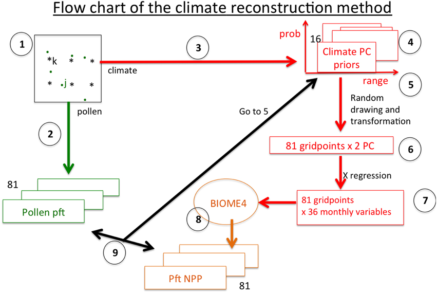
Figure 4. Flow chart of the method described from point 1 to 9. k is the index of gridpoints, j the index of pollen sites.

FIGURE 5

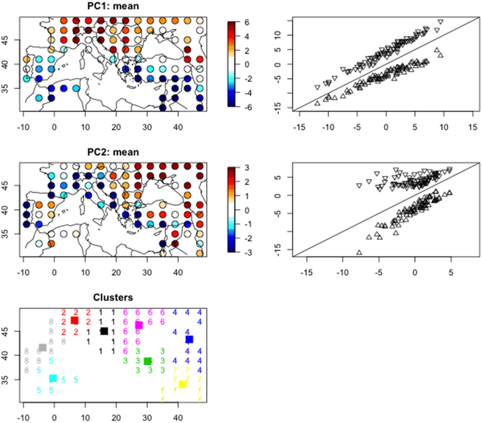
Figure 5. Spatial distribution of the first two principal components used to represent the mean modern climate. At right of these two maps, are represented the lower and upper limits of the priors in function of the mean values (Δ_kj). The lower figure represents the clustering of the gridpoints on the basis of the PC 1 and 2. The numbers give the cluster number and the squares represents the cluster centers.

2.7. Test of Convergence (Test of Gelman and Rubin)

An important problem of the MCMC algorithms is the convergence. Especially when the model is complex, we are never insured that the convergence point (or stationarity) is reached. It exists several procedures to test it (Brooks and Gelman, 1997). One is based on multiple sequences of runs (Gelman and Rubin, 1992). We have defined s = 5 chains of several thousands of iterations starting from random and overdispersed values situated in the range of the prior distribution; we stop when I iterations per sequence are accepted by the algorithm; then we keep for each sequence the last 50% of the values (p = I/2); we calculate the within-chain (W) and between-chain (B) variance of each parameter θ and the estimated variance of each parameter is deduced from them:

$\begin{array}{cc}W=\frac{1}{s}{\displaystyle \sum _{j=1}^s{S}_j^2}with{S}_j^2=\frac{1}{p-1}{\displaystyle \sum _{i=1}^p{w}_i{({\theta }_{ij}-\overline{{\theta }_j})}^2}& \left(4\right)\end{array}$

S²_j is the weighted variance of the j^th chain, θ_j is the weighted mean of the j^thchain. The weight w_j is inversely proportional to the $\widehat{LH}$_i of the iteration i and is then proportionnally to the quality of the fit. W, the mean of the variances of each chain, likely underestimates the true variance of the stationary distribution since our chains have probably not reached all the points of the stationary distribution. B is the variance of the chain means multiplied by p because each chain is based on p draws:

$\begin{array}{cc}B=\frac{p}{s-1}{\displaystyle \sum _{i=1}^s{({\overline{\theta }}_j-\overline{\overline{\theta }})}^2}with\overline{\overline{\theta }}=\frac{1}{s}{\displaystyle \sum _{i=1}^s\overline{{\theta }_j}}& \left(5\right)\end{array}$

We can then estimate the variance of the stationary distribution as a weighted average of W and B

$\begin{array}{cc}\widehat{Var}(\theta )=(1-\frac{1}{p})W+\frac{1}{p}B& \left(6\right)\end{array}$

Because of overdispersion of the starting values, this overestimates the true variance, but is unbiased if the chains have converged. To decide if the s sequences of runs have sufficiently converged, we calculate the potential scale reduction factor:

$\begin{array}{cc}\widehat{R}=\sqrt{\frac{\widehat{Var}(\theta )}{W}}& \left(7\right)\end{array}$

When $\widehat{R}$ is high, typically greater than 1.1, we have to run the chains longer to improve convergence to a stationary distribution. The posterior distributions are finally the combination of the p * s draws. An example of chains obtained for the Gaussian error variance LH parameter, i.e., a measure of the quality of fit between pollen pft and simulated NPP, is shown in Figure 6. The upper panel of tis figure shows that there is a relative coherence between the LH which tends to increases with the number of iterations. The lower panel shows that the coherency between the five chains has a high variability before iteration 1500, with values often >1.01 and stabilized around the value 1.009 after iteration 1500. This value is ≪1.1 and, according to the rule of Gelman and Rubin (1992), it can be accepted.

FIGURE 6

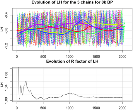
Figure 6. Upper panel: evolution of the likelihood (LH) for the 5 chains in function of the number of iterations (in this test we have continued the iterations until I = 2000). In dashed line, the raw values, in continuous lines, the smoothed values. Lower panel: evolution of the between chain variance of LH in function of the number of iterations (for each iteration, we calculate the variance between the 5 values), given by $\widehat{R}$(θ) where θ = LH in Equation (7).

2.8. Cluster Analysis

The comparison of the climate reconstruction to the twentieth century climate is based on a cluster analysis coupled to a discriminant analysis. First, the 100 yearly vectors of the 81 grid-points for temperature are represented by their first principal component (PC), which explains 41% of the variance, and the 100 yearly vectors of the 81 grid-points for precipitation are transformed into five PCs that explain 52% of the variance. These six PCs are bound and analyzed by a K-means clustering technique (Hartigan and Wong, 1979). The 100 years are clustered into four groups on the basis of their positions in the space of the 6 PCs. The cluster centers are back-transformed into monthly temperature and precipitation to analyze the climate characteristics of the clusters.

The same method is applied to the reconstructions. Vectors of gridded temperature and precipitation are bound for each time step of the last 10,000 years; they are scaled by the standard deviations of the twentieth century time-series, and projected onto the PCs of the twentieth century. Using a linear discriminant analysis (Venables and Ripley, 2002), each vector is assigned to the closest cluster of the twentieth century. This analysis calculates the probability that a reconstructed time slice belongs to each of the four clusters. The cluster with the highest probability is assigned to the time slice.

3. Results

3.1. Reconstruction of the Present Time Slice

The method is illustrated and tested on the time slice [0, 100] year BP, which contains 441 pollen spectra (out of the 16,474 available ones). They correspond to 112 different sites. So, in mean, four spectra/site are dated within this time-interval. We use a CO₂ concentration of 340 ppmv.

The number of accepted iterations is I = 2000 with 5 sequences. For each iteration, the inversion process consists in (i) randomly drawing 16 parameters, (ii) transforming them into 81 gridpoints × 36 climatic variables, (iii) applying BIOME4 to each of the gridpoints, and (iv) simulating the NPP's of the 13 pft's, comparing these NPP's to pollen pft's (after standardization). The iteration is kept if it is sufficiently close from pollen data according to the MCMC rule and is used to increment the posterior histograms.

Two approaches are available to assess the quality of the reconstructions. The first one is based on the prior and posterior distributions. In the Bayesian framework, the information contained in the priors is refined by the data and the model. Consequently, the posterior confidence intervals must be narrower than the prior ones. It is illustrated in Figure 7. The intervals are decreased by 29–72%, with a mean reduction of 57%. It must be denoted that the priors were defined as informative and nevertheless the reduction is high.

FIGURE 7

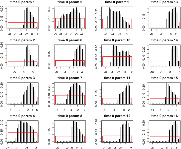
Figure 7. Histograms of the priors and posteriors of the sixteen parameters for gridpoint 62 (5°E, 45°N) for the [0, 100] years BP time-slice. Red rectangles represent the prior distributions and black bars represent the posterior distributions.

The second one is based on the measure of the correlation coefficient between the reconstructed and the observed maps. It is applied on the seven aboved mentionned climatic variables : mean temperature of the coldest month (MTCO), sum of precipitation between April and September (Psum), actual over potential evapotranspiration ratio (E/PE), precipitation minus actual evapotranspiration (P-E), growing degree days over 5°C (GDD5), mean annual temperature (TANN), total annual precipitation (PANN). Table 1 shows that all the reconstructions significantly fit the observed maps. It is notable that E/PE and P-E have the lowest R² because of the particular distribution of the two variables. Figure 8 compares the reconstructed maps of annual temperature and precipitation established on the basis of the prior distributions and on the basis of the posterior distributions. This figure shows that there are some biases in the prior maps: underestimation of southeast temperature and overestimation of northwest. The underestimation of southeast extends on the whole posterior map, except northwest. Looking at the posterior vs. observation graphics, we see that the high MTCO temperature (above 2°C) and high summer precipitation (above 500 mm, 9 points) are underestimated. Precipitation is mainly underestimated on the Atlantic side of the area and in the mountaneous sites; temperature is understestimated almost everywhere but mainly in the south. The fact that gridpoints are often located at lower elevation than pollen sites induces an underestimation of temperature. This explains also the overestimation of precipitation in some points.

TABLE 1

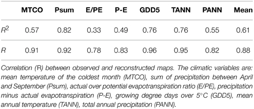
Table 1. Relative variance explained (R²) of the observed climatic fields (maps) by the reconstructed ones.

FIGURE 8

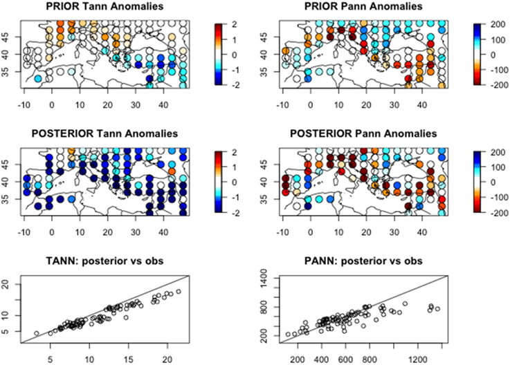
Figure 8. Reconstructed maps of the main climatic variables (mean annual temperature and total annual precipitation) for the present time: the values are given in anomalies from the 1960–1990 averages. The prior maps are given by the mean of the prior uniform distributions, the posterior maps are given by the mean of 5 chains, as indicated in Equation (5). The two bottom panels represent the posterior reconstructions in fonction to the observations; the line represents the perfect reconstruction.

In conclusion, there are systematic biases in the reconstructions due to discrepancies between pollen site and gridpoint elevations. We will correct these biaises in the reconstructions of the past data by calculating the anomalies not according to modern gridpoint climate, but reconstructed climate for the modern time slice.

3.2. Application to the Last 10,000 Years

We applied the method to the 0–10,000 year BP data by increment of 100 years, giving reconstructed maps covering 100 years. We run 5 chains of 1000 accepted iterations. The atmospheric CO₂ concentration is provided by data of Figure 3. The results are extensively displayed in Appendix 2 for 6 climatic variables: MTCO, Psum, P-E, GDD5, TANN, PANN. The variables are expressed in term of anomlies according to their present reconstructions (0–100 years BP). The size of the dots is related to their uncertainties, i.e., the standard deviation of the estimates. Largest circles are used for anomalies three times their standard deviation and dots when they are lower than one standard deviation. The resolution of 100 years is certainly not reached for all the pollen diagrams used in the reconstruction. It is rather a maximum resolution. In reality, the time-series at that time step are rather smoothed and it should be unrealistic to interpret events with a length inferior to several centuries.

We have summarized the results with a principal component analysis of the 81 time-series of the annual temperature and the 81 time-series of the annual precipitation. The first compoenent, even if it explain only 11% of the total variance, enables to summarise the main patterns of the reconstructions. The exteme years along this PC are represented by the set {1200, 4300, 6600, …} years BP and {1300, 3100, 7600, …} years BP. The average annual temperature and precipitation of these years are shown in Figure 9. From the precipitation side, the opposition is clearly between a west and east. From the temperature side, the opposition concerns the area between Italy and Balkans. The years with low precipitation in southeast have a tendency to be warm on Italy and Balkans. At the opposite side, the years which are cold on Balkans are rather wet on the west Mediterranean and slightly dry on east Mediterranean. This shows that the Mediterranean Basin was far to be homogeneous, with three main regions: (1) near East, Turkey, Greece, (2) North Africa, Spain, (3) Italy, Central Europe.

FIGURE 9

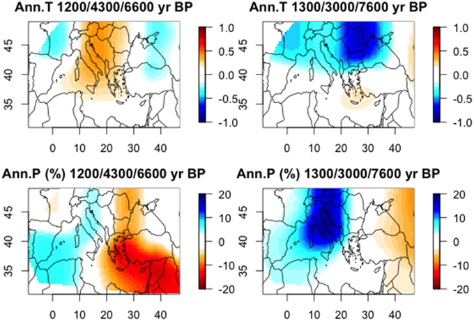
Figure 9. Annual temperature (anomalies in °C) and precipitation (anomalies in %) patterns of two sets of 3 years representing both sides of the first principal component (PC) analysis of the 81 time-series (0–10 k years BP by steps of 100 years) of the annual temperature and precipitation, i.e., 11% of the variance.

3.3. Comparison of the Reconstructions to Twentieth Century

The comparison of the reconstruction with the twentieth century observations is based on cluster and discrimant analysis. Figures 10A,B shows the mean annual temperature and precipitation of these clusters. Cluster K1 represents the hottest (particularly in the north) and driest years (particularly in the south). The time-series of the probabilities to belong to that cluster (Figure 11A) indicate that six of the 8 years belonging to this cluster are found at the end of the twentieth century, and are markers of the recent warming. Cluster K2 corresponds to most of the cold years, particularly in the north. Precipitation anomalies for this cluster were in average close to zero. Figure 10A indicates that they were most probable during the first half of the twentieth century and during 1960–1980. Cluster K3 corresponds to the dry conditions in the northern Mediterranean and the wet conditions in the south. The temperature anomalies were, on average, close to zero. The years belonging to this cluster were equally distributed between 1920 and 1990 (Figure 11A). Cluster K4 is the opposite of cluster K3. K4 corresponds to dry conditions in the southern Mediterranean and wet conditions in the north. The years belonging to K4 were generally warm, particularly in the east and were distributed between 1915 and 1995 (Figure 11A).

FIGURE 10

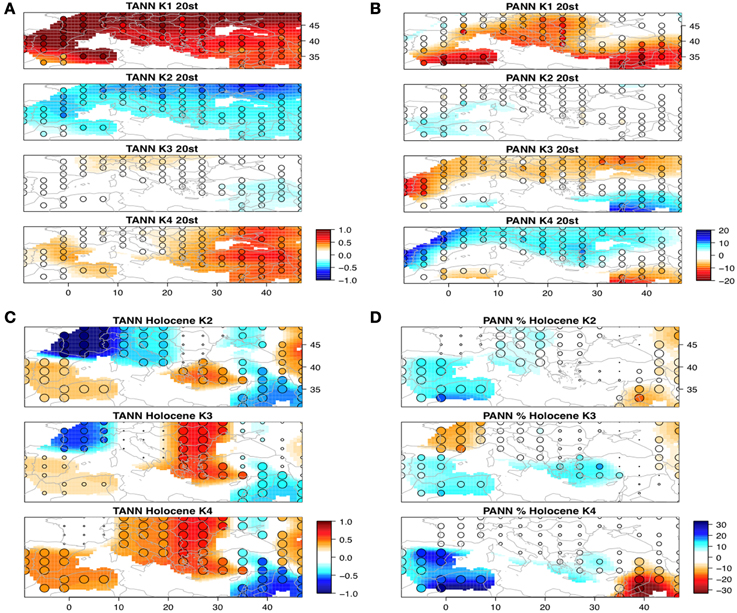
Figure 10. Characteristic climate of the four clusters K1–K4. They are obtained by calculating the climate anomalies averages and standard deviations (vs. the 1960–1990 period) over the observations belonging to the cluster. The colors indicate the amplitude of the average anomalies. The size of circles indicates the average over standard deviations: large circles are used when the anomaly is larger than 2 standard deviations in absolute value, medium circles when it is larger than 1 standard deviation, otherwise small circles. (A) annual temperatures (°C) of the observations of the twentieth century, years (B) annual precipitation (mm/year) of the observations of the twentieth century years, (C) annual temperatures (°C) of the Holocene 100-years time periods, (D) annual precipitation (mm/year) of the Holocene 100 years time periods. 100 year means can be compared to 1 year means because the 100 years values are rescaled to have that same variance than the annual values.

FIGURE 11

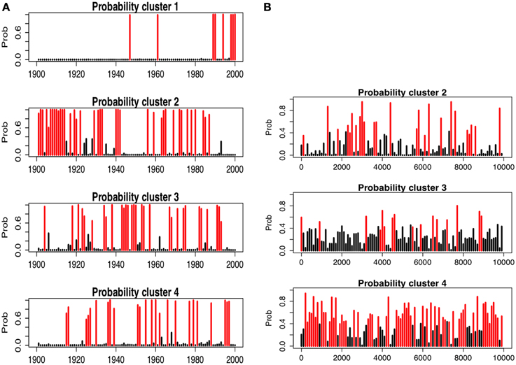
Figure 11. Time series of the probabilities to belong to the clusters K1 to K4. For each cluster, the bars are colored into black if the cluster is not assigned to the time period and into red if it is (i.e., this with the maximum probability). (A) for the annual observations of the twentieth century, (B) for the reconstructed 100-yr time-periods.

The same method is applied to the reconstructions. The reconstructed time series of gridded temperature and precipitation are scaled by the standard deviations of the twentieth century time-series, and projected onto the PCs of the twentieth century. This rescaling is necessary to facilitate the comparison of 100 year means to annual values. Using a linear discriminant analysis (Venables and Ripley, 2002), each vector is assigned to the closest cluster of the twentieth century (Figures 10C,D). This analysis calculates the probability that a reconstructed time period belongs to each of the four clusters. The cluster with the highest probability is assigned to the time period. The temperature and precipitation of the reconstructed time periods belonging to the same cluster are averaged in Figures 10C,D. Figure 11B provides the probability that the reconstructed periods to belong to the four clusters defined on the twentieth century time series. The red bars indicates the maximum probabilities and then the cluster to which the time period belongs. Table 2 gives the sizes of the clusters.

TABLE 2

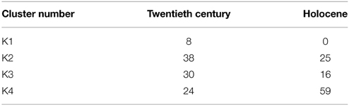
Table 2. Size of the four clusters for the 20th century observations and for the last 10,000 years BP reconstructions, i.e. the number of 20th century years and the number of reconstructed 100 year periods assigned to each cluster.

Three main features emerge from this clustering. The first feature is that cluster K1 (hottest and driest years) is not represented during the last 10,000 years. Therefore, the recent warming, which is nearly equally distributed across the Mediterranean Basin during most of the last decade of the twentieth century (see map of K1 in Figure 10A), had no analog over the last 10,000 years. Even when the recent warming magnitude was reached and or surpassed in areas of the Mediterranean during the last 10,000 years, the warming was not spatially uniform, in contrast to the observed distribution over the last decade. The second feature is the contrast between the southeast and southwest Mediterranean Basin during the last 10,000 years. Clusters K2 and K4 (Figures 10C,D) represent the periods when the climate was wet and warm in the southwest and cool and dry in the southeast. Cluster K3 represents the contrast between the wet south and dry north. The sum of the probabilities of K2 and K4 occurences then reflects the probability of changing to a dry east and a wet west (Figure 12). The third prominent feature is that the last 10,000 years were chiefly dominated by a wetter climate compared with the current values, particularly in the east.

FIGURE 12

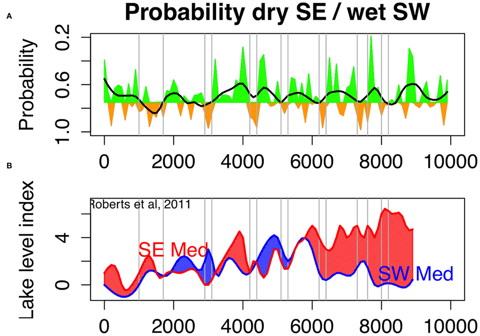
Figure 12. Drought indices for eastern and western Mediterranean. (A) Cumulated probabilities to belong to cluster K2 or K4, representing wet southwest and dry southeast during the last 10,000 years. Note that the y-axis is reversed. Probabilities higher than 0.75 are indicated with orange color and lower than 0.75 with green color. The thick black line represents the millennial trend. (B) reconstruction of lake level index from stacked and normalized lake isotope records (19), five sites for the SW Mediterranean region, seven sites for the SE Mediterranean region; the curves are interpolated at the 100 years time-step to facilitate matching with the pollen reconstruction.

The periods impacted by strong hydrological anomalies in the eastern Mediterranean and western Asia during the last 10,000 years, as indicated by a probability exceeding 0.75 during at least two centuries on the K2–K4 curve (Figure 12A), most of them correspond to well-identified coeval cultural shifts, with drought events at 8200, 5200, 4200, and 3200 years BP. These periods were generally culturally disruptive due to socio-economic declines, transitions from urbanized to rural hamlets, abandonment of territories and migrations of peoples whose native lands were under major water stress (deMenocal et al., 2005; Staubwasser and Weiss, 2006; Weiss and Bradley, 2013). Reduced rainfall and irregularities in water supplies of the initial villages, and later of complex cities, led to an unsustainable decline in rainfed cereal agriculture, food shortages, famine, land abandonment and migration of peoples in search of more fertile plains. They correspond also to a strong see-saw pattern between east and west Mediterranean regions.

4. Discussion

4.1. Climatic Implications

The opposition between southeast and southwest Mediterranean Basin is well identified in the Mediterranean climatology and is one of the variability modes of winter precipitation (Xoplaki et al., 2004) connected with a negative North Atlantic Oscillation (NAO). This mode is characterized by relatively high pressures over Greenland/Iceland and low pressures over southwestern Europe and indicates a weakening of the zonal atmospheric circulation on Europe. The consequence is “above normal precipitation over most of the Mediterranean region with highest values at the western coasts of the peninsulas and lowest at the southeastern part of the basin” (Xoplaki et al., 2004). The southward shifts of storm tracks from Western Europe toward the Mediterranean and vice-versa that in combination with the local cyclogenesis produce the dipole precipitation pattern. Roberts et al. (2012) showed that this mode was also dominant during the Medieval Climate Anomaly (Eleventh to Thirteenth Centuries), dry on west Mediterranean and wetter on East Mediterranean, and during the Little Ice Age (Fifteenth to Nineteenth Centuries) with an opposite pattern.

The reconstruction of the dipole probability (Figure 12A) shows that the first part of the Holocene until approximately 6000 years BP was dominated by wet spells in SE and dry spells in SW, with a probability index frequently lower than 0.75. The low frequency reconstruction of Roberts et al. (2011) based on 12 cores (Figure 12B) generally suggests similar fact. The following period (6000–3300 years BP) remains wet with a probability index generally below 0.75, but the reconstruction of Roberts et al. (2011) seems to indicate that the climate was wet as well in SW than in SE, even if in the latter, there is a significant decrease of precipitation according to the previous period. The last period (3300 years BP to the Present) is clearly drier than before with a probability index generally higher than 0.75, as in Roberts et al. (2011). According to our reconstruction, the maximum aridity seems to have occurred between the Roman Period (1650 years BP) to the end of the Early Middle Ages (900 years BP). This wet-to-dry trend, in which 3300–3200 years BP is the chronological threshold, does not seem to be an outcome of millennial changes but rather fits with the shifts in the relative frequencies of centennial wet-dry periods. Before 3300 years BP, wet periods were more frequent, whereas dry periods became dominant during 3200–1000 years BP (Figure 12).

The climate dynamics during the twentieth century differ from those recorded for the last ten millennia in many respects. The past periods that were marked by long episodes of drought were consistently linked with relatively cool temperatures, as compared with those of the end of the twentieth century. The recent droughts are different because they are amplified by higher temperatures and near-surface evapotranspiration, particularly during the end of the twentieth century (Figure 11). Therefore, the recent warming has had no equivalent over the last 10,000 years. Considering that the spatial distribution of the recent warming is quite uniform compared with the warming recorded during the past 10,000 years in the Mediterranean, the fate of the population seems to be intimately linked to the warming and drying of their lands. People will probably experience an important decline of water quality, severe water shortages mainly in inland territories (Kafle and Bruins, 2009), a loss of ecosystem services, and a human desertification of the driest areas. These additional characteristics seem to indicate that the recent warming in the Mediterranean and Southern Europe is an unprecedented phenomenon at the millennial scale.

4.2. Social Impacts

The 8200 years BP drought event (with a probability value of 0.86, Figure 12A) was supposedly a key factor for the spread of the Neolithic culture to the western Mediterranean and the Black Sea region due to the long-distance migration of populations (Weninger et al., 2006). Large villages were probably converted to small settlements as essential agricultural water was depleted. The 5200 years BP event (with a probability value of 0.84, Figure 12A) corresponds to the collapse of the Late Uruk colony across Greater Mesopotamia (Weiss, 2000) due to a decline in Anatolian precipitation, which was the major water source for the Tigris-Euphrates Rivers (Cullen et al., 2000). A significant decline in precipitation also caused the 4200 years BP event, which is characterized by a probability of 0.96 (Figure 12A). In response, the Harappan civilization appeared to transitioned from an urbanized to a rural society around the Indus valley, whereas the Palestinian cities vanished, leaving only a few villages and towns that were near surface water (Dever, 1995). Across the northern Mesopotamian Habur Plains, a massive desertion of the Akkadian imperialized landscape was identified in which the total population dramatically declined, significant sites were abandoned, and the occupied area greatly decreased (Staubwasser and Weiss, 2006). At 3200 years BP, drought (characterized by a probability value of 0.97, Figure 12A) seems to have hastened the fall of the Old World by inducing famine, invasions and conflicts, leading to the political, economic and cultural chaos termed the “Late Bronze Age collapse” (Kaniewski et al., 2008, 2013; Langgut et al., 2013).

At 2600 years BP, the decline of the Neo-Assyrian Empire, termed “Late Assyrian dry phase”, has been recently attributed (Schneider and Adali, 2014) to a synergy between a severe drought that hit the Middle Tigris valley in northern Iraq and a strong population increase, which reduced significantly the drought resilience. A letter from an influential priest in Assur, Akkulanu, and addressed to the Assyrian king Assurbanipal, is the primary source that provides a glimpse of the impacts, and gives details about this severe drought (Kaniewski et al., 2008; Kuzucuoğlu et al., 2011) in the Assyrian heartland (Parpola and Reade, 1993). Our reconstruction indicates a probability of dry SE of about 0.89 for the Late Assyrian dry phase (Figure 12A). A last dry episode has been recently highlighted for the period 3700–3600 years BP, during the reign of the Babylonian King Abieshuh. Cuneiform tablets from Iraq, which correspond to the oldest known written evidence of the diversion of the Tigris for repression purposes, show that the king attempted to dry up the Mesopotamian Marshes in order to starve southern Iraq during a period marked by recurrent dry spells (Kaniewski et al, submitted.). Our reconstruction indicates a probability of dry SE of about 0.75 (Figure 12A).

Speleothems and pollen data show two clear dry phases during the historical period in Anatolia, the first around 300–550 CE, the other around 750–900 CE (Haldon et al., 2014). The first one corresponded to increased drought and famine frequencies. The second one, less dry, was nevertheless marked by land abandonment, reduced farming and forest recovery. The re-occupation of Cappadocia between 850 and 950 CE coincided with a wetter climate, suggesting that a better agroclimatic environment may have encouraged the re-establishment of the middle Byzantine rural economy.

Natural drought probably accentuated the impact of deliberate water retention on human settlement and population migrations. As the Mesopotamian marshes turned to desert, marsh peoples were forced to flee their homes. These events suggest that during the Holocene, populations faced climate pressures that forced them to either adapt or migrate. This assumption is based on an important concept: a threshold exists for which adjustments become impossible.

Relation between societies and climate is certainly complex and we do certainly not want to explain societal changes by climate only. Even in the present time with higher technological event, a combination of unsustainable agriculture and precipitation deficit may trigger a succession of political problems as in Syria (Kelley et al., 2015). Different interpretations have been given of what has been considered as a collapse of societies: from a simple explanation though environmental mismanagement (Diamond, 2005), to a more elaborate one based on an inefficient complexification of the society (Tainter, 1990). Many collapses may be best seen as representing the consequences of conflicts between and within groups, which may have been triggered or exacerbated by a wide range of both internal and external causes with unpredictable consequences (Middleton, 2012). Complexification, especially in terms of activities, is then considered to be societies' way of responding to the changing environment, as they try to solve problems related to an increasing scarcity of their resources. It is also the cause of their collapse when, in economic terms, the marginal returns on investment in complexity start diminishing.

Funding

Labex OT-Med (ANR-11-LABEX-0061), “Investissements d'Avenir,” French Government project of the French National Research Agency (ANR), A*Midex project (ANR-11-IDEX-0001-02). French National Research Agency ANR-12-SENV-0008-01, GEOMAR program.

Author Contributions

JG performed the research and wrote the manuscript. DK provided six pollen sites and significantly contributed to write the context and the discussion of the results. DK revised and approved the final manuscript.

Conflict of Interest Statement

The authors declare that the research was conducted in the absence of any commercial or financial relationships that could be construed as a potential conflict of interest.

Acknowledgments

This work is a contribution to the program MISTRALS/PALEOMEX. Support to DK was provided by the Institut Universitaire de France and the CLIMSORIENT program. Pollen data have been obtained from the European Pollen Data (EPD) and belong to multiple authors (more than one hundred). The data have been extracted for this study by Michèle Leydet, the engineer in charge of the data. Extraction software is maintained by Armand Rotereau.

Supplementary Material

The Supplementary Material for this article can be found online at: https://www.frontiersin.org/article/10.3389/feart.2015.00028/abstract

References

Brayshaw, D. J., Rambeau, C. M. C., and Smith, S. J. (2011). Changes in mediterranean climate during the holocene: insights from global and regional climate modelling. Holocene 21, 15–31. doi: 10.1177/0959683610377528

CrossRef Full Text | Google Scholar

Brooks, S., and Gelman, A. (1997). General methods for monitoring convergence of iterative simulations. J. Comput. Graph. Stat. 7, 434–455.

Google Scholar

Cullen, H. M., deMenocal, P. B., Hemming, S., Hemming, G., Brown, F. H., Guilderson, T., et al. (2000). Climate change and the collapse of the akkadian empire: evidence from the deep sea. Geology 28, 379–382. doi: 10.1130/0091-7613(2000)28<379:CCATCO>2.0.CO;2

CrossRef Full Text | Google Scholar

Davis, B. A. S., Brewer, S., Stevenson, A. C., Guiot, J., and Data Contributors. (2003). The temperature of europe during the holocene reconstructed from pollen data. Q. Sci. Rev. 22, 1701–1716. doi: 10.1016/S0277-3791(03)00173-2

PubMed Abstract | CrossRef Full Text | Google Scholar

deMenocal, P. B. (2001). Cultural responses to climate change during the late holocene. Science 292, 667–673. doi: 10.1126/science.1059827

PubMed Abstract | CrossRef Full Text | Google Scholar

deMenocal, P. B., Cook, E. R., Demeritt, D., Hornborg, A., Kirch, P. V., McElreath, R., et al. (2005). Perspectives on diamond's collapse: how societies choose to fail or succeed. Curr. Anthropol. 46, S91–S99. doi: 10.1086/497663

CrossRef Full Text | Google Scholar

Dever, W. (1995). Social Structure in the Early Bronze IV Period in Palestine. New York, NY: Facts on File.

Diamond, J. (2005). Collapse: How Societies Choose to Fail or Succeed. New York, NY: Viking Penguin.

Evans, J. P. (2009). 21st century climate change in the middle east. Clim. Change 92, 417–432. doi: 10.1007/s10584-008-9438-5

CrossRef Full Text | Google Scholar

Evans, J. P., Smith, R. B., and Oglesby, R. J. (2004). Middle east climate simulation and dominant precipitation processes. Int. J. Climatol. 24, 1671–1694. doi: 10.1002/joc.1084

CrossRef Full Text | Google Scholar

Garreta, V., Miller, P. A., Guiot, J., Hely, C., Brewer, S., Sykes, M. T. et al. (2010). A method for climate and vegetation reconstruction through the inversion of a dynamic vegetation model. Clim. Dyn. 35, 371–389. doi: 10.1007/s00382-009-0629-1

CrossRef Full Text | Google Scholar

Gasse, F., and Roberts, C. N. (2004). “Late quaternary hydrologic changes in the arid and semiarid belt of northern Africa - implications for past atmospheric circulation,” in RS Conference on the Hadley Circulation – Present, Past and Future, vol. 21 (Dordrecht: Springer), 313–345.

Gelman, A., and Rubin, D. (1992). Inference from iterative simulation using multiple sequences. Stat. Sci. 7, 452–472. doi: 10.1214/ss/1177011136

CrossRef Full Text | Google Scholar

Giorgi, F. (2006). Climate change hot-spots. Geophys. Res. Lett. 33, L08707. doi: 10.1029/2006GL025734

CrossRef Full Text | Google Scholar

Giorgi, F., and Lionello, P. (2008). Climate change projections for the mediterranean region. Glob. Planet. Change 63, 90–104. doi: 10.1016/j.gloplacha.2007.09.005

CrossRef Full Text | Google Scholar

Guiot, J., Boucher, E., and Gea-Izquierdo, G. (2014). Process models and model-data fusion in dendroecology. Front. Ecol. Evol. 2:52. doi: 10.3389/fevo.2014.00052

CrossRef Full Text | Google Scholar

Guiot, J., Torre, F., Jolly, D., Peyron, O., Borreux, J., and Cheddadi, R. (2000). Inverse vegetation modeling by Monte Carlo sampling to reconstruct paleoclimate under changed precipitation seasonality and CO2 conditions: application to glacial climate in mediterranean region. Ecol. Modell. 127, 119–140. doi: 10.1016/S0304-3800(99)00219-7

CrossRef Full Text | Google Scholar

Guiot, J., Wu, H. B., Garreta, V., Hatte, C., and Magny, M. (2009). A few prospective ideas on climate reconstruction: from a statistical single proxy approach towards a multi-proxy and dynamical approach. 5, 571–583. doi: 10.5194/cp-5-571-2009

CrossRef Full Text | Google Scholar

Haldon, J., Roberts, N., Izdebski, A., Fleitmann, D., McCormick, M., Cassis, M., et al. (2014). The climate and environment of byzantine anatolia: Integrating science, history, and archaeology. J. Interdiscipl. Hist. 45, 113–161. doi: 10.1162/JINH_a_00682

CrossRef Full Text | Google Scholar

Hartigan, J., and Wong, M. A. (1979). Algorithm as 136: a k-means clustering algorithm. J. R. Stat. Soc. C Appl. Stat. 28, 100–108. doi: 10.2307/2346830

CrossRef Full Text | Google Scholar

Haslett, J., Whiley, M., Bhattacharya, S., Salter-Townshend, M., Wilson, S., Allen, J., et al. (2006). Bayesian paleoclimate reconstruction. J. R. Stat. Soc. A 169, 395–438. doi: 10.1111/j.1467-985X.2006.00429.x

PubMed Abstract | CrossRef Full Text | Google Scholar

Hastings, W. (1970). Monte Carlo sampling methods using Markov chains and their application. Biometrika 57, 97–109. doi: 10.1093/biomet/57.1.97

CrossRef Full Text | Google Scholar

Haxeltine, A., and Prentice, I. (1996). Biome3: an equilibrium terrestrial biosphere model based on ecophysiological constraints, resource availability and competition among plant functional types. Glob. Biogeochem. Cycles 10, 693–709. doi: 10.1029/96GB02344

CrossRef Full Text | Google Scholar

Indermühle, A., Stocker, T., Joos, F., Fischer, H., Smith, H., Wahlen, M., et al. (1999). Holocene carbon-cycle dynamics based on CO2 trapped in ice at taylor dome, Antarctica. Nature 398, 121–126. doi: 10.1038/18158

CrossRef Full Text | Google Scholar

Kafle, H., and Bruins, H. (2009). Climatic trends in israel 1970–2002: warmer and increasing aridity inland. Clim. Change 96, 63–77. doi: 10.1007/s10584-009-9578-2

CrossRef Full Text | Google Scholar

Kaniewski, D., Paulissen, E., van Campo, E., Al-Maqdissi, M., Bretschneider, J., and van Lerberghe, K. (2008). Middle east coastal ecosystem response to middle-to-late holocene abrupt climate changes. Proc. Natl. Acad. Sci. U.S.A. 105, 13941–13946. doi: 10.1073/pnas.0803533105

PubMed Abstract | CrossRef Full Text | Google Scholar

Kaniewski, D., van Campo, E., Morhange, C., Guiot, J., Zviely, D., Shaked, I., et al. (2013). Early urban impact on mediterranean coastal environments. Sci. Rep. 3:3540. doi: 10.1038/srep03540

PubMed Abstract | CrossRef Full Text | Google Scholar

Kaplan, J., Prentice, N. B. I., Harrison, S., Bartlein, P., Christensen, T., Cramer, W., et al. (2003). Climate change and arctic ecosystems: 2. modeling, paleodata-model comparisons, and future projections. J. Geophys. Res. Atmos. 108, 8171. doi: 10.1029/2002JD002559

CrossRef Full Text | Google Scholar

Kelley, C. P., Mohtadi, S., Cane, M. A., Seager, R., and Kushnir, Y. (2015). Climate change in the fertile crescent and implications of the recent syrian drought. Proc. Natl. Acad. Sci. U.S.A. 112, 3241–3246. doi: 10.1073/pnas.1421533112

PubMed Abstract | CrossRef Full Text | Google Scholar

Korhola, A., Vasko, K., Toivonen, H., and Olandor, H. (2002). Holocene temperature changes in northern fennoscandia reconstructed from chironomids using Bayesian modelling. Q. Sci. Rev. 21, 1841–1860. doi: 10.1016/S0277-3791(02)00003-3

CrossRef Full Text | Google Scholar

Kuzucuoğlu, C., Dörfler, W., Kunesch, S., and Goupille, F. (2011). Mid-to late-holocene climate change in central turkey: the tecer lake record. Holocene 21, 173–188. doi: 10.1177/0959683610384163

CrossRef Full Text | Google Scholar

Langgut, D., Finkelstein, I., and Litt, T. (2013). Climate and the late bronze collapse: new evidence from the southern levant. Tel. Aviv. 40, 149–175. doi: 10.1179/033443513X13753505864205

CrossRef Full Text | Google Scholar

Lionello, P., Platon, S., and Rodo, X. (2008). Preface: trends and climate change in the mediterranean region. Glob. Planet. Change 63, 87–89. doi: 10.1016/j.gloplacha.2008.06.004

CrossRef Full Text

Lobell, D. B., Burke, M. B., Tebaldi, C., Mastrandrea, M. D., Falcon, W. P., and Naylor, R. L. (2008). Prioritizing climate change adaptation needs for food security in 2030. Science 319, 607–610. doi: 10.1126/science.1152339

PubMed Abstract | CrossRef Full Text | Google Scholar

Metropolis, N., Rosenbluth, A., Rosenbluth, M., Teller, A., and Teller, E. (1953). Equations of state calculations by fast computing machines. J. Chem. Phys. 21, 1087–1093. doi: 10.1063/1.1699114

CrossRef Full Text | Google Scholar

Middleton, G. (2012). Nothing lasts forever: environmental discourses on the collapse of past societies. J. Archaeol. Res. 20, 257–307.

Google Scholar

Parpola, S., and Reade, J. (1993). Letters from Assyrian and Babylonian Scholars, Vol. 10. Helsinki: Helsinki University Press.

Prentice, C., Guiot, J., Huntley, B., Jolly, D., and Cheddadi, R. (1996). Reconstructing biomes from palaeoecological data: a general method and its application to european pollen data at 0 and 6 ka. Clim. Dyn. 12, 185–194. doi: 10.1007/BF00211617

CrossRef Full Text | Google Scholar

Prentice, I., and Harrison, S. (2009). Ecosystem effects of CO2 concentration: evidence from past climates. Clim. Past 5, 297–307. doi: 10.5194/cp-5-297-2009

CrossRef Full Text | Google Scholar

Reuveny, R. (2007). Climate change-induced migration and violent conflict. Polit. Geogr. 26, 656–673. doi: 10.1177/0959683610388058

CrossRef Full Text | Google Scholar

Robert, C., and Casella, G. (2013). Monte Carlo Statistical Methods (New York, NY: Springer Science & Business Media), 649.

Google Scholar

Roberts, N., Brayshaw, D., Kuzucuoglu, C., Perez, R., and Sadori, L. (2011). The mid-holocene climatic transition in the mediterranean: causes and consequences. Holocene 21, 3–13. doi: 10.1177/0959683610388058

CrossRef Full Text | Google Scholar

Roberts, N., Moreno, A., Valero-Garces, B. L., Corella, J. P., Jones, M., Allcock, S., et al. (2012). Palaeolimnological evidence for an east-west climate see-saw in the mediterranean since AD 900. Glob. Planet. Change 84-85, 23–34. doi: 10.1016/j.gloplacha.2011.11.002

CrossRef Full Text | Google Scholar

Schneider, A. W., and Adali, S. F. (2014). No harvest was reaped: demographic and climatic factors in the decline of the neo-assyrian empire. Clim. Change 127, 435–446. doi: 10.1007/s10584-014-1269-y

CrossRef Full Text | Google Scholar

Sowers, J., Vengosh, A., and Weinthal, E. (2011). Climate change, water resources, and the politics of adaptation in the middle east and north Africa. Clim. change 104, 599–627. doi: 10.1007/s10584-010-9835-4

CrossRef Full Text | Google Scholar

Staubwasser, M., and Weiss, H. (2006). Holocene climate and cultural evolution in late prehistoric-early historic west asia - introduction. Q. Res. 66, 372–387. doi: 10.1016/j.yqres.2006.09.001

CrossRef Full Text | Google Scholar

Stocker, T., Qin, D., Plattner, G.-K., Tignor, M., Allen, S., Boschung, J., et al. (2013). Climate Change 2013: The Physical Science Basis. Contribution of Working Group I to the Fifth Assessment Report of the Intergovernmental Panel on Climate Change. Cambridge: Cambridge University Press.

Tainter, J. (1990). The Collapse of Complex Societies. Cambridge: Cambridge University Press.

Google Scholar

Tarasov, P., Cheddadi, R., Guiot, J., Bottema, S., Peyron, O., Belmonte, J., et al. (1998). A method to determine warm and cool steppe biomes from pollen data; application to the mediterranean and Kazakhstan regions. J. Q. Sci. 13, 335–344.

Google Scholar

Trigo, R. M., Gouveia, C. M., and Barriopedro, D. (2010). The intense 2007-2009 drought in the fertile crescent: impacts and associated atmospheric circulation. Agric. For. Meteorol. 150, 1245–1257. doi: 10.1016/j.agrformet.2010.05.006

CrossRef Full Text | Google Scholar

Venables, W. N., and Ripley, B. D. (2002). Modern Applied Statistics with S. New York, NY: Springer-Verlag.

Google Scholar

Weiss, H. (2000). Beyond the Younger Dryas: Collapse as Adaptation to Abrupt Climate Change in Ancient West Asia and the Eastern Mediterranean. University of New Mexico Press, Albuquerque.

Weiss, H. (2001). What drives societal collapse? Science 291, 609–610. doi: 10.1126/science.1058775

PubMed Abstract | CrossRef Full Text | Google Scholar

Weiss, H., and Bradley, R. (2013). “What drives societal collapse?,” in The Anthropology of Climate Change: An Historical Reader, ed M. R. Dove (New York, NY: John Wiley & Sons), 151.

Weninger, B., Alram-Stern, E., Bauer, E., Clare, L., Danzeglocke, U., Joeris, O., et al. (2006). Climate forcing due to the 8200 cal yr bp event observed at early neolithic sites in the eastern mediterranean. Q. Res. 66, 401–420. doi: 10.1016/j.yqres.2006.06.009

CrossRef Full Text | Google Scholar

Wu, H. B., Guiot, J., Brewer, S., Guo, Z. T., and Peng, C. H. (2007). Dominant factors controlling glacial and interglacial variations in the treeline elevation in tropical africa. Proc. Natl. Acad. Sci. U.S.A. 104, 9720–9724. doi: 10.1073/pnas.0610109104

PubMed Abstract | CrossRef Full Text | Google Scholar

Xoplaki, E., Gonzalez-Rouco, J. F., Luterbacher, J., and Wanner, H. (2004). Wet season mediterranean precipitation variability: influence of large-scale dynamics and trends. Clim. Dyn. 23, 63–78. doi: 10.1007/s00382-004-0422-0

CrossRef Full Text | Google Scholar

Zaitchik, B. F., Evans, J. P., Geerken, R. A., and Smith, R. B. (2007). Climate and vegetation in the middle east: interannual variability and drought feedbacks. J. Clim. 20, 3924–3941. doi: 10.1175/JCLI4223.1

CrossRef Full Text | Google Scholar