The pattern across the continental United States of evapotranspiration variability associated with water availability

Introduction

Meteorological variables (e.g., precipitation and air temperature) vary across multiple time scales. Seasonal-to-interannual variations in these variables can manifest themselves in many ways—as an abnormally hot summer, for example, or as a crippling drought. Understanding the mechanisms underlying such long-term variability is a critical first step toward predicting societally-relevant variations well ahead of time and quantifying societal vulnerabilities to such variations in the face of climatic shifts.

The time scales of atmospheric processes are generally not amenable to the maintenance of seasonal meteorological anomalies. For such long time scales, other, slower-moving components of the climate system must come into play. Oceanic heat anomalies, for example, vary at long time scales; the prediction of oceanic variations and their consequent impacts on atmospheric variations at long leads underlies today's operational seasonal forecasting efforts (e.g., Kirtman et al., 2014).

Soil moisture is another slower-moving climate system component, with residence times of order weeks to months (Vinnikov and Yeserkepova, 1991; Entin et al., 2000); it thus has the potential to contribute to monthly or seasonal predictions (e.g., Koster et al., 2011). For summer in midlatitudes (the focus of this paper), soil moisture indeed has the potential to contribute more skill to seasonal forecasts than can ocean conditions (Koster et al., 2000). The primary conduit by which soil moisture variations can induce variations in atmospheric variables and thus aid in prediction is through its control over the evapotranspiration rate and, by extension, through its control over the surface energy balance as a whole (e.g., the generation of sensible heat and concomitant impacts on boundary layer growth, etc.). A basic understanding of how interannual variations in soil moisture are communicated to the atmosphere thus requires a characterization of the interannual behavior of evapotranspiration and how it is controlled by the availability of water in the soil.

This paper aims to provide such a characterization. More specifically, it aims to quantify the spatial pattern over the continental United States (U.S.) of the interannual variability of May–September total evapotranspiration, focusing in particular on that part of the variability associated with variations in water availability (see Section Methods: Water-dependent Evapotranspiration Variability). That is, we aim to determine where this variance is large and thus potentially relevant to land-atmosphere feedback, as well as where it is small, suggestive of little feedback. Such information is not easily accessible in the literature.

Here we quantify the spatial pattern of water-dependent evapotranspiration variance through analysis of observations-based datasets, avoiding estimates obtained through numerical climate modeling or reanalysis, since they necessarily reflect numerous modeling assumptions and associated model biases. This focus on observations, however, imposes an important caveat to our study. Given a dearth of relevant soil moisture observations, we instead characterize water availability in this paper with contemporaneous and antecedent precipitation (see Section Methods: Water-dependent Evapotranspiration Variability). We are, in essence, assuming a first order relationship between soil moisture and precipitation, with high (low) precipitation leading to high (low) soil moisture. This required assumption must be kept in mind when interpreting our results in the context of land-atmosphere feedback. Also, note that we focus here solely on the U.S., mainly because it is a large continental region with multiple hydroclimatic regimes and because it is, for the most part, well-instrumented throughout.

We look first at the interannual variability inherent in two multidecadal, gridded estimates of evapotranspiration available in the literature (Section Analysis of Gridded Evapotranspiration Datasets). Recognizing that these datasets, though observations-based, do not represent direct measurements of evapotranspiration itself and are thus inherently uncertain, we follow this up (Section Analysis of Relevant Proxy Variables) with the analysis of the water-dependent interannual variance of three independent proxy variables (namely, temperature, streamflow, and normalized difference vegetation index, or NDVI), each of which should show variability patterns mimicking those of evapotranspiration. The agreement in the patterns across all of the datasets, while not perfect, is remarkably strong, providing confidence that the main patterns generated are accurate. For additional context, we provide in the discussion section (Section Discussion) an analysis of the evapotranspiration variability implied by the hydroclimatic analysis framework of Budyko (1974).

Methods: Water-dependent Evapotranspiration Variability

Evapotranspiration, E, is controlled by more than just moisture availability. Interannual variations in evapotranspiration can also reflect interannual variations in incident radiation, wind speed, temperature of incoming advected air, and so on. Because, however, we are particularly interested in evapotranspiration as the conduit linking soil moisture variability with meteorological variability, we seek in this paper to quantify the evapotranspiration variability specifically associated with moisture availability.

Water-dependent evapotranspiration variability is quantified here with σ²_E*, the statistically-derived portion of the total interannual evapotranspiration variance that is “explained” by variations in the availability of moisture for evapotranspiration. We define σ²_E* as:

$\begin{array}{cc}{\sigma }^2{{}_{\text{E}}}^{*}={\sigma }^2{}_{\text{E}}{\text{r}}^2\left(E,W\right),& (1)\end{array}$

where σ²_E is the total variance of E and r²(E,W) is the square of the correlation coefficient between E and W, the variable used to represent moisture availability. We thus employ the standard interpretation of r²(E,W) as the fraction of the variance of E “explained” by variations in W (It can be shown, in fact, that if E is regressed on W, so that E is approximated with the linear equation E_est = aW+b, then σ²_E* is the variance of the resulting E_est values). Equation (1) effectively allows us to isolate the water-dependent part of evapotranspiration variability from that associated with other sources, such as variations in radiation or humidity.

Again, our focus here is on the warm season in the U.S., the period when evapotranspiration should be largest. The E-values used in the calculation of σ²_E and r²(E,W) at a given location are the evapotranspirations averaged over May through September (MJJAS), one value per year in a given dataset. The W-values would optimally be the corresponding MJJAS root zone soil moisture averages, one value per year; however, we avoid using soil moisture here because direct measurements of root zone soil moisture do not exist across the U.S. over multiple decades and because model-generated soil moisture products, while widely available, reflect model-specific assumptions regarding soil moisture's connection to evapotranspiration, something we want to avoid. We instead rely on precipitation, a relatively well-observed variable, to characterize moisture availability. For W in Equation (1) we use the observed precipitation averaged over April–September. The connection between soil moisture and contemporaneous or slightly antecedent precipitation (indicated here by our inclusion of April precipitation) follows largely from mass balance considerations (larger precipitation amounts wet the soil more) and is well established in the literature (e.g., Pan et al., 2003; Brocca et al., 2014).

In using precipitation for W in the term r²(E,W), we test for positive values of r, which would be consistent with a causal impact of precipitation on water supply and thus on evaporation. Negative values of r are zeroed because, if they don't result from sampling error, they may reflect irrelevant connections. For example, due to cloudiness, total warm season precipitation may be negatively correlated with average warm season net radiation, which would be positively correlated with E [so that r(E,W) would be negative], or the precipitation may be positively correlated with humidity, which would be negatively correlated with E [so that again, r(E,W) would be negative]. In our analyses, statistically significant negative correlations in fact turn out to be rare.

In this paper, unless otherwise stated, the precipitation data used are from the high quality Climate Prediction Center (CPC) U.S. Unified Precipitation dataset (Chen et al., 2008a,b). These data, along with the evapotranspiration estimates examined, are gridded to a resolution of 2.5°×2.5° to emphasize large scale patterns in σ²_E*.

Results

Analysis of Gridded Evapotranspiration Datasets

While some direct observations of land surface evapotranspiration are obtained, for example, with lysimeters or eddy correlation systems, these measurements are too sparse to allow the direct quantification of evapotranspiration and its variability across continental scales. Investigators thus use alternative means to quantify continental-scale evapotranspiration. Estimates, for example, can be obtained by driving a land surface model across the continent with observations-based meteorological forcing (e.g., Dirmeyer et al., 2006). While model-derived estimates can be useful, we avoid using them here specifically because the simulated rates reflect built-in assumptions regarding the sensitivity of evapotranspiration to variations in soil moisture. We also avoid the use of satellite-based estimates of evapotranspiration (e.g., Ferguson et al., 2010), as these estimates rely on many of their own algorithmic assumptions and because they do not provide the multiple decades of data needed to characterize interannual variability.

There are, however, gridded estimates of evapotranspiration spanning multiple decades that are strongly tied to observations and that do not rely on assumed evapotranspiration-soil moisture relationships. In this section, we quantify the σ²_E* values inherent in two such datasets.

ETRHEQ-based Evapotranspiration Product

The Rigden and Salvucci (2015) evapotranspiration dataset was derived from meteorological data using a method based on the relationship between the diurnal cycle of relative humidity and evapotranspiration (Salvucci and Gentine, 2013)—a method known as “ETRHEQ” (evapotranspiration based on relative humidity at equilibrium). Specifically, Salvucci and Gentine (2013) found that the surface conductance to water vapor transport, the key rate-limiting parameter of typical evapotranspiration models, can be estimated as the value that minimizes the vertical variance of the calculated relative humidity profile averaged over the day. The key advantage of this approach is that biophysical and hydrological surface parameters (stomatal conductance, soil texture, soil moisture, etc.) are not required to estimate evapotranspiration. Evapotranspiration estimates instead require diurnal measurements of five meteorological variables: screen height air temperature, humidity, wind speed, pressure, and downwelling shortwave radiation.

To estimate evapotranspiration across the U.S., Rigden and Salvucci (2015) applied the method at 305 weather stations for 50 years (1961–2010). The procedure involved adjusting the weather station data to match PRISM (Parameter-elevation Relationships on Independent Slopes Model) estimates (Daly et al., 2008) for the given month to mitigate site-specific bias in temperature and humidity and to improve the data's continuity over the period of record. Vegetation height (needed to characterize the surface roughness length) was inferred from satellite-derived land cover data. Sub-daily evapotranspiration estimates were temporally averaged to monthly values at each station. To create the gridded evapotranspiration dataset from the station-based estimates, Rigden and Salvucci (2015) spatially interpolated the average monthly evapotranspiration estimates to a 0.25°×0.25° grid using the ANUSPLIN software package (Hutchinson, 1995; Hutchinson and Xu, 2007), which interpolates using a multivariate thin-plate smoothing spline. Land cover data was also used in the interpolation.

For this study, the gridded ETRHEQ-based evapotranspiration data from Rigden and Salvucci (2015) were aggregated spatially to 2.5°×2.5° and were temporally averaged, for each year during the period 1961–2010, over the period May–September. Using these yearly MJJAS values and corresponding April–September values of precipitation from the CPC U.S. Unified dataset, we computed, at each 2.5°×2.5° grid cell, the values of σ²_E and r²(E,W), which are shown in Figures 1A,B. The interannual variance of MJJAS evapotranspiration is strongest in the west, as is the square of the correlation between evapotranspiration and water availability.

FIGURE 1

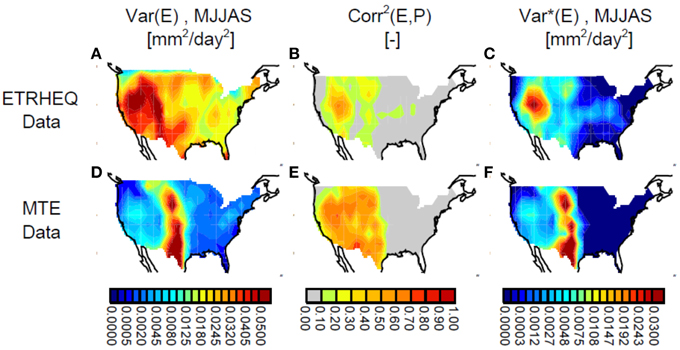
Figure 1. (A) Variance of MJJAS evapotranspiration, σ²_E, as determined from the evapotranspiration dataset of Rigden and Salvucci (2015). (B) Square of the correlation coefficient, Corr²(E,P), between MJJAS evapotranspiration from the dataset of Rigden and Salvucci (2015) and April–September precipitation [referred to in text as r²(E,P)]. (C) σ²_E*, or the product of σ²_E and Corr²(E,P), as derived from the dataset of Rigden and Salvucci (2015). (D–F) Same as (A–C), but for the dataset of Jung et al. (2010).

The σ²_E and r²(E,W) values are shown in the figure mostly for background; the quantity of chief interest here is their product, σ²_E*, shown in Figure 1C. It too is largest in the west. The diagnostic indeed shows a large maximum lying in the far west, but not touching the coast; secondary maxima appear to indicate high values along a north–south swath down the center of the U.S. In the eastern half of the U.S., water-dependent evapotranspiration variance is very small.

MTE-based Evapotranspiration Product

The product of Jung et al. (2010, 2011) is based on an empirical approach that combines monthly eddy covariance evapotranspiration observations from about 200 FLUXNET sites (Baldocchi et al., 2001), remotely sensed measurements of FAPAR (fraction of absorbed photosynthetically active radiation), and meteorological variables in a machine learning approach called Model Tree Ensembles (MTE, Jung et al., 2009). The density of the FLUXNET sites used is largest in North America (the focus of this paper) and Europe. While more than 40 predictor variables were used to train the MTE, only three of them vary interannually and thus contribute directly to the interannual variance of E: precipitation, temperature, and FAPAR. The interannual variance of the MTE-based ET product appears to be underestimated (Jung et al., 2011).

As with the ETRHEQ-based evapotranspiration estimates, the data of Jung (covering 1982–2008) were aggregated temporally and spatially to MJJAS totals at 2.5°×2.5°. Figures 1D–F shows the corresponding derived values of σ²_E, r²(E,W), and σ²_E*. The quantities show some interesting differences with the ETRHEQ-based values. The interannual variance of MJJAS evapotranspiration (Figure 1D) is maximized along the aforementioned north–south swath down the center of the U.S., with low values seen in the west, and the r²(E,W) values in Figure 1E are similar in pattern to those in Figure 1B but with larger magnitudes.

Again, though, the diagnostic of chief importance for us is the water-dependent MJJAS evapotranspiration variance, which is shown in Figure 1F. This variance is very clearly maximized along the north–south swath, with no large maximum in the far west. The differences in the two σ²_E* fields are particularly interesting because the ETRHEQ-based and MTE-based evapotranspiration products were found by Rigden and Salvucci (2015) to be similar in terms of annual means and mean seasonal cycles across the U.S. Figure 1 suggests that this similarity in means does not imply a corresponding level of similarity in interannual variability.

Analysis of Relevant Proxy Variables

The σ²_E* patterns from the two evapotranspiration datasets (Figures 1C,F) show both similarities (e.g., the low values in the east and higher values in the middle of the U.S.) and differences (particularly in the west). We note again that neither plot is based on direct evapotranspiration measurements; such direct measurements spanning the continent over multiple decades do not exist. Given this uncertainty, we now explore further the σ²_E* pattern that actually exists in nature by looking at the signal inherent in proxy geophysical variables, each of which has been well measured over multiple decades across the U.S., and each of which has a variability that is strongly tied to that of evapotranspiration. The three proxy variables we consider here are air temperature, streamflow, and NDVI.

By direct analogy with Equation (1), we define the water-dependent interannual variance of a given proxy variable X as

$\begin{array}{cc}{\sigma }^2{{}_{\text{X}}}^{*}={\sigma }^2{}_{\text{X}}{\text{r}}^2\left(X,W\right)& (2)\end{array}$

where σ²_X is the total variance of X and r²(X,W) is the square of the correlation coefficient between X and W. As before, W is taken to be precipitation averaged over April–September, except (as discussed below) when the proxy variable involves streamflow.

Temperature

In contrast to directly measured evapotranspiration data, air temperature data are abundant. The connection between seasonally-averaged near-surface air temperature and seasonally-averaged evapotranspiration is conceptually well-established (Seneviratne et al., 2010). Put simply, in water-limited evapotranspiration regimes, higher (lower) evapotranspiration rates lead to increased (decreased) evaporative cooling of the land surface and thereby to reduced (increased) surface air temperature, particularly given that synoptic variability is averaged out through the seasonal averaging. Accordingly, areas with higher evapotranspiration variance should have larger air temperature variance. Again, this is particularly true in areas for which soil moisture variations control evapotranspiration rates, which are the regions of interest in this paper. In wetter regimes, other effects come into play; evapotranspiration, controlled by energy availability, can co-vary positively in these regions with air temperature. An earlier study (Koster et al., 2006a) used a set of atmospheric model experiments to show that observed temperature variances do seem to reflect these mechanisms; those findings are, in effect, expanded here through the use of the water-dependent variance calculation, Equation (2).

The air temperature data used here are from the Global Historical Climatology Network (GHCN) station dataset (Peterson and Vose, 1997). We examined all stations within North America that satisfy two constraints: (i) the existence of at least 30 years of MJJAS air temperature values, and (ii) the coexistence of monthly GHCN precipitation data for the same years, for either the same site or for a station within a few kilometers of the site. For the temperature analysis, we indeed use these GHCN precipitation data rather than the CPC gridded precipitation data to compute W. The average MJJAS air temperature, T, is the variable X in Equation (2).

Figures 2A–C show the associated spatial patterns of σ²_T, r²(T,W), and σ²*_T. Values are plotted as color-coded circles at each measurement station's location. The precise magnitudes of σ²_T and σ²_T* are not shown because our only aim here is to provide the spatial pattern of evapotranspiration variability—all variance values within a given plot are scaled by a map-specific factor to allow the patterns to be compared directly to those for the other, correspondingly scaled proxy variables.

FIGURE 2

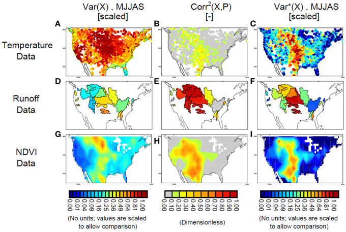
Figure 2. (A) Variance of MJJAS air temperature, σ²_T, as determined from GHCN air temperature data. (B) Square of the correlation coefficient, Corr²(T,P), between MJJAS air temperature and April–September precipitation. (C) σ²_T*, or the product of σ²_T and Corr²(T,P). (D–F) Same as (A–C), but for the difference between annual basin-averaged precipitation and annual basin-averaged streamflow, and with the correlations computed against annual precipitation. (G–I) Same as (A-C), but for NDVI data averaged over August–September.

The temperature data show a total variance that is largest in the center of the country but is still large toward either coast. The square of the correlation between T and P, however, is decidedly maximized in the swath down the center of the country, and thus σ²_T* is also maximized along this swath, with values close to zero toward either coast. The σ²_T* pattern in Figure 2C, a proxy for the evapotranspiration pattern we are seeking in this paper, is strongly reminiscent of that found for the Jung et al. (2010) data in Figure 1F.

Streamflow

The second data type examined is streamflow, which has an obvious connection to evapotranspiration: annual evapotranspiration in a region is roughly equal to the annual precipitation in the region minus the annual streamflow generated in the region, with any imbalance associated with (assumed small) changes in yearly soil moisture storage. Furthermore, annual evapotranspiration is a strong indicator of MJJAS evapotranspiration, since the warm season produces by far the most evapotranspiration in most areas (For example, the average May–September evapotranspiration over the U.S. from the ETRHEQ data set is over four times that of the average November–March evapotranspiration). Here we examine streamflow data from 23 gauged basins in the continental United States. The streamflow data cover at least 39 years and generally exceed 60 years; see Table 2 in Mahanama et al. (2012) for a full description of the basins examined and their associated data. For precipitation, we use the gauge-based dataset constructed by Andreadis et al. (2005) rather than the CPC U.S. Unified Dataset because two of the basins extend outside of the continental U.S. and because the former dataset goes back further in time, allowing more of the streamflow measurements to be utilized.

Note that several of the monitored basins are “nested” within others. In this paper, if Basin B, for example, is nested within Basin A, results for Basin A refer only to that part of Basin A that does not include Basin B. In other words, before any other calculations are performed, the measured annual streamflow, Q, examined for Basin A is transformed as follows:

$\begin{array}{cc}{Q}_{\text{BasinA}\prime }=Q_{\text{BasinA}}-Q_{\text{BasinB}}.& (3)\end{array}$

We correspondingly define P_BasinA, the precipitation for Basin A, to be the annual precipitation falling on the portion of Basin A that does not include Basin B.

For streamflow, the quantity X in Equation (2) for Basin N is P_BasinN–Q_BasinN, which, again, assumes that interannual variations in storage can be neglected. Note that in addition we apply an area-dependent scaling factor to σ²_P−Q* to account for differences in basin size—all things being equal, a larger basin will show lower variability than a smaller basin simply due to the more extensive “averaging out” of spatial variability within the former. The applied scaling factor aims to convert a computed P–Q variance into the corresponding value for a smaller interior basin of a specific nominal size (as would be computed if such small-scale streamflow measurements were available), thereby allowing the results from the disparately-sized basins to be directly compared. The scaling factors are derived from the factors relevant to the precipitation data covering the basin. If Basin A contains N small grid cells, the scale factor, S, for P–Q is computed as

$S_{\text{Basin}\text{A}}=\frac{(1/N){\displaystyle {\sum }_{n=1,N}{\sigma }^2}(P_n)}{{\sigma }^2(P_{BasinA})}$

where σ²(P_n) is the variance of precipitation in grid cell n, and σ²(P_BasinA) is the variance of the basin-averaged precipitation. While the statistical properties of P–Q will differ from those of P, use of Equation (4) is deemed much more sensible than either ignoring the impact of area on variance (i.e., setting S_BasinA to 1) or assuming that P–Q in the different N grid cells are spatially uncorrelated (i.e., setting S_BasinA to N). Equation (4) offers the best estimate of S_BasinA possible given available data.

One final note about the processing of the streamflow data is needed: because we are working with annual totals of precipitation and runoff (shorter averaging periods make no sense for estimating evaporation from P and Q, given interseasonal storage of moisture, Milly, 1994), we use here the annual (October–September) precipitation rather than the April–September precipitation for W in Equation (2). As an aside, we computed the spatial distributions (not shown) of warm season water-dependent variances for the other variables (ETRHEQ-based evaporation, air temperature, etc.) using annual precipitation instead of April–September precipitation for W and found very little impact on the results, presumably because most of the annual precipitation across the U.S. falls during the warm season. We could thus have used annual precipitation for the other variables as well, producing essentially the same plots.

The streamflow-based results are presented in Figures 2D–F, with basins color-coded according to the value of the quantity considered in each plot. The primary difference between the streamflow results and those of the other data sources considered so far is the very high level of correlation between P–Q and P in Figure 2E, which is not surprising given that the two quantities are not independently measured. The pattern of r²(P–Q, P) in Figure 2E has the effect of transforming the pattern of σ²(P–Q) in Figure 2D, which shows a weak maximum of variance down the center of the country, into the much more pronounced swath of high values for σ²_P−Q* in Figure 2F. In strong agreement with the temperature-based results, the streamflow-based analysis shows that in general, evapotranspiration variability associated with moisture variations is maximized along a swath down the center of the continent. The swaths for T and P–Q are indeed co-located; they both even show a slant to the northwest in their northern sections. One distinction does exist, however: for the streamflow-based data, values in the northern part of the swath are smaller than those in the southern part. Even so, the values in the northern part are still, in general, substantially larger than those toward either coast.

Normalized Difference Vegetation Index

The final proxy variable considered here is satellite-based NDVI data, variations of which reflect variations in the lushness, or leafiness, of vegetation. Rather than assuming a simple cause-and-effect relationship between NDVI and evapotranspiration (higher NDVI implies more leaves and thus greater transpiration), we consider both evapotranspiration and NDVI as acting in response to moisture availability—low soil moisture during the warm season leads to both a low warm season evapotranspiration and to a reduced greenness of vegetation by the end of summer, when the initially reduced water stores have been depleted and vegetation becomes water-stressed and less green. Support for this interpretation—and thus for the consideration of late-summer NDVI rather than NDVI averaged over MJJAS for the calculation of σ²_NDVI*—comes from calculations (not shown) indicating that correlations between NDVI and antecedent precipitation are relatively low in May and June and are highest across the continent in August (See also Figure 5 of Zeng et al., 2013).

The NDVI data used in this analysis is the Global Inventory Modeling and Mapping Studies data, or GIMMS (Tucker et al., 2005). The data's native resolution is 8 km and semiweekly, and the data used here span the period July 1982–2008. The data are derived from the Advanced Very High Resolution Radiometer (AVHRR) instrument with known limitations compared to the more advanced MODIS instrument (Kaufman et al., 1998). However, the longer temporal coverage of GIMMS relative to MODIS (29 vs. 11 years) and the good correspondence between their measurements (Tucker et al., 2005; Beck et al., 2011) makes it well suited to the analysis presented here. We aggregate the data to 2.5°×2.5°, again in order to highlight large-scale structures in variance. The term X and W in Equation (2) are taken to be, respectively, the NDVI averaged over August–September (AS) and the corresponding April–September precipitation.

Results are shown in Figures 2G–I. Values of r²(NDVI,P) are high in the west and low in the east (Figure 2H), and the raw variance of AS NDVI is small in the west and larger in the east (Figure 2G). Only in the center of the country, down the now-familiar north–south swath, are both values high, leading to a pattern of σ²_NDVI* (Figure 2I) very similar to that found for temperature and streamflow and that found for the Jung et al. (2010) data. As before, the magnitudes of the variances are not shown, the focus here being on spatial pattern—particularly the spatial pattern of σ²_NDVI*.

Discussion

All three proxy variables (air temperature, streamflow, and NDVI) support certain findings from the analysis of the two gridded evapotranspiration datasets, namely, that water-dependent evapotranspiration variance is small in the eastern half of the U.S. and large in a long swath stretching northward from western Texas. The large maximum of σ²_E* seen in the far west for the ETRHEQ-based evapotranspiration data (Figure 1C) does not appear in the proxy data, though the proxy data do show some hints of larger-than average values in the region. Note that the strength of the western maximum in Figure 1C could also stem from data limitations in the Western U.S. The ETRHEQ-based gridded evapotranspiration dataset is based on data collected at long-term weather stations, which tend to be located in low elevation, populated regions. The evapotranspiration estimates in the Western U.S. are therefore based on relatively few stations. In addition, although elevation and land cover data were used to spatially interpolate the station evapotranspiration across the U.S., capturing the evapotranspiration dynamics in the topographically complex Western U.S. may require a more robust spatial interpolation method (see e.g., Daly, 2006) than used here.

A word about data independence is warranted. The three proxy variables in section Analysis of Relevant Proxy Variables represent independent measurements, and thus Figures 2C, F, I are indeed independent estimates of the distribution of σ²_E*. The two evaporation products examined in Section Analysis of Gridded Evapotranspiration Datasets, however, are not as independent. As noted above, the MTE-based evapotranspiration data have an interannual variability that reflects the interannual variability of the input variables temperature, precipitation, and FAPAR (which in turn is strongly related to NDVI), and this explains in large part the similarities of the σ²_E* patterns in Figure 1F with those in either Figure 2C or Figure 2I. Accordingly, the MTE-based evapotranspiration results are not presented here as an independent estimate of the σ²_E* pattern. While their presence here is arguably redundant, they nevertheless represent a unique and learned combination of the NDVI and temperature data. The ETRHEQ-based data are perhaps more independent of the proxy variables, since they depend largely on independent relative humidity measurements.

Note that the spatial pattern of water-dependent evapotranspiration variance could alternatively be computed from output of numerical climate models or from reanalyses—either full atmospheric reanalyses (e.g., Dee et al., 2011) or output from land data assimilation systems (e.g., Mitchell et al., 2004). Any patterns so obtained, however, would be subject to assumptions and biases in the land models producing the data and, certainly for the free-running atmospheric models, to biases in the simulated climate. By avoiding the use of climate models and their land model components in this analysis, we have in fact generated a pattern that could serve as a useful validation target for the models. For a climate model to capture properly the connection between soil moisture and the atmosphere at seasonal time scales and thus the corresponding impacts of soil moisture on interannual climate variability, it must capture the indicated pattern in σ²_E*. (We repeat, however, our caveat that we used precipitation rather than soil moisture to characterize water availability). Analyses of simulated feedback with observations are rare (though see Dirmeyer et al., 2006), largely due to the scarcity of useful observational targets.

The σ²_E* pattern also has relevance, for example, to determining where in situ soil moisture measurements and/or satellite-based soil moisture measurements [e.g., from the Soil Moisture Ocean Salinity (Kerr et al., 2010) and Soil Moisture Active Passive (Entekhabi et al., 2010) missions] may be most useful for atmospheric forecasts—usefulness should increase where evaporation variations are more strongly connected to water variability. It may even have relevance to water management, given that higher σ²_E* values imply lower values of streamflow variability, all else being equal.

Why does the spatial pattern of σ²_E* look as it does? From the time of Budyko (1974), energy availability rather than water availability has been assumed to control evapotranspiration rates in wetter areas; this is consistent with the small values of σ²_E* seen in the east. In the dry west, water availability does control evapotranspiration, but water variations—and thus evapotranspiration variations—are small. According to such arguments, only in the middle of the U.S. does water-limited evapotranspiration combine with a large interannual variability in water abundance to produce large values of σ²_E*. This thinking underlies various interpretations of evapotranspiration variability in climate models (Guo et al., 2006). It is used to explain the positions of “hotspots” of land-atmosphere feedback (i.e., regions for which prescribed variations in soil moisture induce predictable variations in precipitation and air temperature) uncovered in the multi-model analysis of Koster et al. (2004). The North American hotspot in that study is indeed similar to the north–south swaths for σ²_E* seen in Figures 1, 2.

For further context, it is interesting to compare the results above to those obtained through the application of Budyko's decades-old hydroclimatic framework. Using energy and water balance considerations in conjunction with existing empirical relationships, Budyko (1974) characterized the ratio of annual evapotranspiration E to annual precipitation P in terms of the dryness index R_net/λP, where R_net is the annual net radiation and λ is the latent heat of vaporization of water:

$\begin{array}{c}\text{E}/\text{P}=\{\left({\text{R}}_{\text{net}}/\text{P}\lambda \right)\text{tanh}\left(\text{P}\lambda /{\text{R}}_{\text{net}}\right)[1-\text{cosh}\left({\text{R}}_{\text{net}}/\text{P}\lambda \right)\\ +{\text{sinh}\left({\text{R}}_{\text{net}}/\text{P}\lambda \right)]\}}^{1/2}\\ =\text{F}\left({\text{R}}_{\text{net}}/\text{P}\lambda \right).& (5)\end{array}$

Budyko (1974) showed the equation to be strongly consistent with the hydrological data available to him at that time. Starting from Equation (5), and making the assumption that the interannual variability of λR_net is significantly smaller than that of P, Koster and Suarez (1999) derived an equation for the ratio of interannual evapotranspiration variance σ²_E to interannual precipitation variance σ²_P:

$\begin{array}{cc}{\sigma }_{\text{E}}^2\text{/}{\sigma }_{\text{P}}^2\text{ = }{[\text{F}({\text{R}}_{\text{net}}\text{/P}\lambda )-({\text{R}}_{\text{net}}\text{/P}\lambda )\text{F'}({\text{R}}_{\text{net}}\text{/P}\lambda )]}^{\text{2}}& (6)\end{array}$

where F′(R_net/Pλ) is the derivative of the function F with respect to R_net/Pλ. Koster et al. (2006b) showed that both Equation (5) and Equation (6) are consistent with state-of-the-art estimates of precipitation, net radiation, and streamflow across the globe.

In effect, Equation (6) provides an estimate of σ²_E from precipitation and net radiation data alone. Given the assumptions underlying the semi-empirical framework—particularly the idea that year-to-year variations in evapotranspiration reflect only year-to-year variations in precipitation—the equation by default provides a direct estimate of σ²_E* for annual evapotranspiration and, through the assumption that most evapotranspiration occurs during the warm season, for MJJAS evapotranspiration. Using Equation (6) with the gridded CPC U.S. Unified Precipitation dataset and the net radiation data of Stackhouse et al. (2004) from the Surface Radiation Budget (SRB) project, as described in Koster et al. (2006b), we produce the map of σ²_E* shown in Figure 3.

FIGURE 3

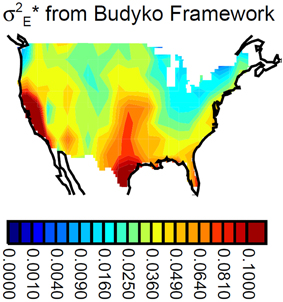
Figure 3. Distribution of σ²_E* (mm²/day²) as derived from the hydroclimatic analysis framework of Budyko (1974).

Budyko's semi-empirical hydroclimatic framework produces σ²_E* patterns with some strong similarities to those derived from the evapotranspiration and proxy variable datasets. The high values along the swath sweeping northward from western Texas are clearly seen, as are low values on either side of the swath, toward either coast. The magnitudes of the variances, however, are much larger than those from the two gridded evaporation datasets (note the different scale on the color bar), partly because, unlike the values derived for the evaporation datasets, the values from the Budyko framework are not reduced by that part of r²(E,W) associated with measurement or representativeness error. Notice also that the Budyko framework produces high values in California that are probably not realistic, since the framework does not deal well with areas for which seasonal precipitation and net radiation maxima are wholly out of phase (Koster et al., 2006b). The Budyko framework does hint at the far west maximum seen in the ETRHEQ-based data (Figure 1C), though the relative magnitude of the maximum is quite a bit lower. Interestingly, the Budyko framework suggests that the σ²_E* values in the north–south swath down the center of the country peter out toward the northern end, a feature captured (to some degree) only by the streamflow data.

Any differences between the pattern in Figure 3 and corresponding σ²_E* patterns in Figures 1, 2 are in fact not a concern, since again, Figure 3 is presented mainly for historical context. The Budyko (1974) framework is an approximate, semi-empirical framework for capturing the broad controls of energy and water availability on evapotranspiration. For this reason, we expect the σ²_E* patterns obtained from the evapotranspiration datasets (Section Analysis of Gridded Evapotranspiration Datasets) and proxy datasets (Section Analysis of Relevant Proxy Variables) to be more accurate than that in Figure 3.

Summary

A common pattern of water-dependent evapotranspiration variance is captured in five separate datasets, most of which are based on wholly independent observations. The robustness of the pattern across the datasets implies that it is representative of the pattern operating in nature: in nature, the variance is high down the center of the North American continent, low in the east, and probably low in the west. While theoretically this pattern is not unexpected (Budyko, 1974; Koster et al., 2004), it is nevertheless reassuring to see this key facet of climate variability and of the global hydrological cycle appear in the observational data.

Conflict of Interest Statement

The authors declare that the research was conducted in the absence of any commercial or financial relationships that could be construed as a potential conflict of interest.

Acknowledgments

We thank Sarith Mahanama and Ben Livneh for help with the processing of the data. This work was supported by NASA's Modeling, Analysis, and Prediction Program.

References

Andreadis, K. M., Clark, E. A., Wood, A. W., Hamlet, A. F., and Lettenmaier, D. P. (2005). Twentieth-century drought in the conterminous United States. J. Hydrometeorol. 6, 985–1001. doi: 10.1175/JHM450.1

CrossRef Full Text | Google Scholar

Baldocchi, D., Falge, E., Gu, L. H., Olson, R., Hollinger, D., Running, S., et al. (2001). FLUXNET, A new tool to study the temporal and spatial variability of ecosystem-scale carbon dioxide, water vapor, and energy flux densities. Bull. Am. Meteorol. Soc. 82, 2415–2434. doi: 10.1175/1520-0477(2001)082

CrossRef Full Text | Google Scholar

Beck, H. E., McVicar, T. R., van Dijk, A. I. J. M., Schellekens, J., de Jeu, R. A. M., and Bruijnzeel, L. A. (2011). Global evaluation of four AVHRR-NDVI data sets, Intercomparison and assessment against Landsat imagery. Remote Sens. Environ. 115, 2547–2563. doi: 10.1016/j.rse.2011.05.012

CrossRef Full Text | Google Scholar

Brocca, L., Ciabatta, L., Massari, C., Moramarco, T., Hahn, S., Hasenauer, S., et al. (2014). Soil as a natural rain gauge, Estimating global rainfall from satellite soil moisture data. J. Geophys. Res. Atmos. 119, 5128–5141. doi: 10.1002/2014JD021489

CrossRef Full Text | Google Scholar

Budyko, M. I. (1974). Climate and Life. New York, NY: Academic Press.

Google Scholar

Chen, M., Shi, W., Xie, P., Silva, V. B. S., Kousky, V. E., Wayne Higgins, R., et al. (2008a). Assessing objective techniques for gauge-based analyses of global daily precipitation. J. Geophys. Res. 113, D04110. doi: 10.1029/2007jd009132

CrossRef Full Text | Google Scholar

Chen, M., Xie, P., and CPC Precipitation Working Group. (2008b). “CPC unified gauge-based analysis of global daily precipitation,” Western Pacific Geophysics Meeting (Cairns, QLD).

Google Scholar

Daly, C. (2006). Guidelines for assessing the suitability of spatial climate data sets. Int. J. Climatol. 26, 707–721. doi: 10.1002/joc.1322

CrossRef Full Text | Google Scholar

Daly, C., Halbleib, M., Smith, J. I., Gibson, W. P., Doggett, M. K., Taylor, G. H., et al. (2008). Physiographically sensitive mapping of climatological temperature and precipitation across the conterminous United States. Int. J. Climatol. 28, 2031–2064. doi: 10.1002/joc.1688

CrossRef Full Text | Google Scholar

Dee, D. P., Uppala, S. M., Simmons, A. J., Berrisford, P., Poli, P., Kobayashi, S., et al. (2011). The ERA-Interim reanalysis: configuration and performance of the data assimilation system. Q. J. R. Meteorol. Soc. 137, 553–597. doi: 10.1002/qj.828

CrossRef Full Text | Google Scholar

Dirmeyer, P. A., Gao, X., Zhao, M., Guo, Z., Oki, T., and Hanasaki, N. (2006). GSWP-2 Multimodel analysis and implications for our perception of the land surface. Bull. Am. Meteorol. Soc. 87, 1381–1397. doi: 10.1175/BAMS-87-10-1381

CrossRef Full Text | Google Scholar

Entekhabi, D., Njoku, E. G., O'Neill, P. E., Kellogg, K. H., Crow, W. T., Edelstein, W. N., et al. (2010). The Soil Moisture Active Passive (SMAP) mission. Proc. IEEE 98, 704–716. doi: 10.1109/JPROC.2010.2043918

CrossRef Full Text | Google Scholar

Entin, J. K., Robock, A., Vinnikov, K. Y., Hollinger, S. E., Liu, S., and Namkhai, A. (2000). Temporal and spatial scales of observed soil moisture variations in the extratropics. J. Geophys. Res. 105, 11865–11877. doi: 10.1029/2000JD900051

CrossRef Full Text | Google Scholar

Ferguson, C. R., Sheffield, J., Wood, E. F., and Gao, H. (2010). Quantifying uncertainty in a remote sensing-based estimate of evapotranspiration over continental USA. Int. J. Remote Sens. 31, 3821–3865. doi: 10.1080/01431161.2010.483490

CrossRef Full Text | Google Scholar

Guo, Z., Dirmeyer, P. A., Koster, R. D., Bonan, G., Chan, E., Cox, P., et al. (2006). GLACE: the global land-atmosphere coupling experiment, Part 2, Analysis. J. Hydromet. 7, 611–625. doi: 10.1175/jhm511.1

CrossRef Full Text | Google Scholar

Hutchinson, M. F. (1995). Interpolating mean rainfall using thin plate smoothing splines. Int. J. Geogr. Inf. Syst. 9, 385–403. doi: 10.1080/02693799508902045

CrossRef Full Text | Google Scholar

Hutchinson, M. F., and Xu, T. (2007). ANUSPLIN Version 4.4 User Guide. Canberra, ACT: The Australian National University, Fenner School of Environment and Society. Available online at: http://fennerschool.anu.edu.au/files/anusplin44.pdf.

Jung, M., Reichstein, M., Ciais, P., Seneviratne, S. I., Sheffield, J., Goulden, M. L., et al. (2010). Recent decline in the global land evapotranspiration trend due to limited moisture supply. Nature 467, 951–954. doi: 10.1038/nature09396

PubMed Abstract | CrossRef Full Text | Google Scholar

Jung, M., Reichstein, M., Margolis, H. A., Cescatti, A., Richardson, A. D., Arain, M. A., et al. (2011). Global patterns of land-atmosphere fluxes of carbon dioxide, latent heat, and sensible heat derived from eddy covariance, satellite, and meteorological observations. J. Geophys. Res. 116, G00J07. doi: 10.1029/2010jg001566

CrossRef Full Text | Google Scholar

Jung, M., Reichstein, M., and Bondeau, A. (2009). Towards global empirical upscaling of FLUXNET eddy covariance observations: validation of a model tree ensemble approach using a biosphere model. Biogeosciences 6, 2001–2013. doi: 10.5194/bg-6-2001-2009

CrossRef Full Text | Google Scholar

Kaufman, Y. J., Herring, D. D., Ranson, K. J., and Collatz, G. J. (1998). Earth observing system AM1 mission to earth. IEEE Trans. Geosci. Remote Sens. 36, 1045–1055. doi: 10.1109/36.700989

CrossRef Full Text | Google Scholar

Kerr, Y. H., Waldteufel, P., Wigneron, J. P., Delwart, S., Cabot, F., Boutin, J., et al. (2010). The SMOS mission: new tool for monitoring key elements of the global water cycle. Proc. IEEE, 98, 666–687. doi: 10.1109/jproc.2010.2043032

CrossRef Full Text | Google Scholar

Kirtman, B. P., Min, D., Infanti, J. M., Kinter, J. L., Paolino, D. A., Zhang, Q., et al. (2014). The North American multi-model ensemble. Bull. Am. Meteorol. Soc. 95, 585–601. doi: 10.1175/BAMS-D-12-00050.1

CrossRef Full Text | Google Scholar

Koster, R. D., Dirmeyer, P. A., Guo, Z., Bonan, G., Chan, E., Cox, P., et al. (2004). Regions of strong coupling between soil moisture and precipitation. Science 305, 1138–1140. doi: 10.1126/science.1100217

PubMed Abstract | CrossRef Full Text | Google Scholar

Koster, R. D., Mahanama, S. P. P., Yamada, T. J., Balsamo, G., Berg, A. A., Boisserie, M., et al. (2011). The second phase of the global land-atmosphere coupling experiment, soil moisture contributions to subseasonal forecast skill. J. Hydrometeorol. 12, 805–822. doi: 10.1175/2011JHM1365.1

CrossRef Full Text | Google Scholar

Koster, R. D., Fekete, B. M., Huffman, G. J., and Stackhouse, P. W. Jr. (2006b). Revisiting a hydrological analysis framework with international satellite land surface climatology project initiative 2 rainfall, net radiation, and runoff fields. J. Geophys. Res. 111, D22S05. doi: 10.1029/2006JD007182

CrossRef Full Text | Google Scholar

Koster, R. D., and Suarez, M. J. (1999). A simple framework for examining the interannual variability of land surface moisture fluxes. J. Climate 12, 1911–1917.

Google Scholar

Koster, R. D., Suarez, M. J., and Heiser, M. (2000). Variance and predictability of precipitation at seasonal-to-interannual timescales. J. Hydrometeorol. 1, 26–46. doi: 10.1175/1525-7541(2000)001

CrossRef Full Text | Google Scholar

Koster, R. D., Suarez, M. J., and Schubert, S. (2006a). Distinct hydrological signatures in observed historical temperature fields. J. Hydrometeorol. 7, 1061–1075. doi: 10.1175/JHM530.1

CrossRef Full Text | Google Scholar

Mahanama, S., Livneh, B., Koster, R., Lettenmaier, D., and Reichle, R. (2012). Soil moisture, snow, and seasonal streamflow forecasts in the United States. J. Hydrometeorol. 13, 189–203. doi: 10.1175/JHM-D-11-046.1

CrossRef Full Text | Google Scholar

Milly, P. C. D. (1994). Climate, soil water storage, and the average annual water balance. Water Resour. Res. 30, 2143–2156. doi: 10.1029/94WR00586

PubMed Abstract | CrossRef Full Text | Google Scholar

Mitchell, K. E., Lohmann, D., Houser, P. R., Wood, E. F., Schaake, J. C., Robock, A., et al. (2004). The multi-institution North American Land Data Assimilation System (NLDAS), Utilizing multiple GCIP products and partners in a continental distributed hydrological modeling system. J. Geophys. Res. 109, D07S90. doi: 10.1029/2003jd003823

CrossRef Full Text | Google Scholar

Pan, F. F., Peters-Lidard, C. D., and Sale, M. (2003). An analytical method for predicting surface soil moisture from rainfall observations. Water Resour. Res. 39, 1314. doi: 10.1029/2003wr002142

CrossRef Full Text | Google Scholar

Peterson, T. C., and Vose, R. S. (1997). An overview of the global historical climatology network temperature database. Bull. Am. Meteorol. Soc. 78, 2837–2849.

Google Scholar

Rigden, A. J., and Salvucci, G. D. (2015). Evapotranspiration based on equilibrated relative humidity (ETRHEQ), Evaluation over the continental United States. Water Resour. Res. 51, 2951–2973. doi: 10.1002/2014WR016072

CrossRef Full Text | Google Scholar

Salvucci, G. D., and Gentine, P. (2013). Emergent relation between surface vapor conductance and relative humidity profiles yields evaporation rates from weather data. Proc. Natl. Acad. Sci. U.S.A. 110, 6287–6291. doi: 10.1073/pnas.1215844110

PubMed Abstract | CrossRef Full Text | Google Scholar

Seneviratne, S. I., Corti, T., Davin, E. L., Hirschi, M., Jaeger, E. B., Lehner, I., et al. (2010). Investigating soil moisture-climate interactions in a changing climate: a review. Earth Sci. Rev. 99, 125–161. doi: 10.1016/j.earscirev.2010.02.004

CrossRef Full Text | Google Scholar

Stackhouse, P. W. Jr. Gupta, S. K., Cox, S. J., Mikovitz, J. C., Zhang, T., and Chiacchio, M. (2004). 12-year surface radiation budget data set. GEWEX News 14, 10–12.

Tucker, C. J., Pinzon, J. E., Brown, M. E., Slayback, D. A., Pak, E. W., Mahoney, R., et al. (2005). An extended AVHRR 8-km NDVI dataset compatible with MODIS and SPOT vegetation NDVI data. Int. J. Remote Sens. 26, 4485–4498. doi: 10.1080/01431160500168686

CrossRef Full Text | Google Scholar

Vinnikov, K. Y., and Yeserkepova, I. B. (1991). Soil moisture, empirical data and model results. J. Climate 4, 66–79.

Google Scholar

Zeng, F.-W., Collatz, G. J., Pinzon, J. E., and Ivanoff, A. (2013). Evaluating and quantifying the climate-driven interannual variability in Global Inventory Modeling and Mapping Studies (GIMMS) Normalized Difference Vegetation Index (NDVI3g) at global scales. Remote Sens. 5, 3918–3950. doi: 10.3390/rs5083918

CrossRef Full Text | Google Scholar