Growth and decay of the equatorial Atlantic SST mode by means of closed heat budget in a coupled general circulation model

Introduction

Tropical Atlantic Variability (TAV) have important impacts over Africa and South America, where rain-fed agriculture is an important part of their economies (Xie and Carton, 2004; Chang et al., 2006a; Kushnir et al., 2006; Rodríguez-Fonseca et al., 2015). However, historically major efforts have been done in understanding the Tropical Pacific which holds the most important inter-annual variability mode in terms of the global impacts: El Niño and the Southern Oscillation (ENSO, Philander, 1990). The Tropical Atlantic (TA) has received much less attention. Recently, scientific community is focusing attention in understanding model biases over the TA, which is systemic and common problem in coupled General Circulation Models (GCM). These biases could have important consequences in the ability of the models in simulating proper tele-connections which could lead to failure in seasonal to decadal forecasts. This paper is focused in understanding how a GCM simulates the main inter-annual variability mode with major impacts in surrounding areas and its systematic errors.

Inter-annual TAV has been described by two main modes: Equatorial Mode or Atlantic Niño and the Meridional Mode (Zebiak, 1993; Carton et al., 1996; Ruiz-Barradas et al., 2000; Kushnir et al., 2006; also see Xie and Carton, 2004; Chang et al., 2006a, for a revision). The Atlantic Niño presents anomalous SST over eastern equatorial Atlantic, it is phase-locked to the seasonal cycle, mainly occurring from June to September season, when the seasonal equatorial cold tongue develops over the eastern Atlantic associated with a northward Inter-Tropical Convergence Zone (ITCZ)-shift and the West African Monsoon (WAM) onset (Sultan et al., 2003; Okumura and Xie, 2004).

The Atlantic Niño mode is therefore tightly associated with the WAM inter-annual variability (Janicot et al., 1998; Ward, 1998; Giannini et al., 2003; Polo et al., 2008; Losada et al., 2010; Rodriguez-Fonseca et al., 2011; Rodríguez-Fonseca et al., 2015): positive (negative) SST anomalies influence the rainfall over the Gulf of Guinea through a decrease (increase) of the local surface temperature gradient, weakening (strengthening) the monsoon flow and the surface convergence over the Sahel (Vizy and Cook, 2001; Losada et al., 2010).

From observations, the origin of the mode has been mainly associated with anomalous equatorial winds over the western equatorial Atlantic (Zebiak, 1993; Latif and Grötzner, 2000; Keenlyside and Latif, 2007) and the evolution of the SST anomalies is related to positive Bjerknes feedback (Keenlyside and Latif, 2007) and Ekman processes (Hu and Huang, 2007). However, oceanic wave eastward propagation could also play a role in the evolution of the SST anomalies in the eastern Atlantic (Latif and Grötzner, 2000; Florenchie et al., 2003) although ocean waves could also be important in damping the mode (Polo et al., 2008). Finally, a recent study from Richter et al. (2012b) has pointed out other sources for the equatorial SST variability in the observations, such as the oceanic advection from the North Tropical Atlantic (NTA).

However, several studies have found that the Atlantic Niño usually starts over the South Atlantic via a weakening of the Sta Helena high pressure system, reaching the equator later on, where it evolves throughout Bjerknes feedback mechanism (Sterl and Hazeleger, 2003; Keenlyside and Latif, 2007; Trzaska et al., 2007; Polo et al., 2008; Lübbecke et al., 2010). In addition, some authors have highlighted the SST dipole pattern between the equator and the south Atlantic as part of a SST feedback trough changes in the Hadley circulation (Nnamchi and Li, 2011; Namchi et al., 2013).

In the observations, the Atlantic Niño generally appears associated with SST anomalies over the coastal Benguela upwelling region, which usually precedes the equatorial anomalies (Hu and Huang, 2007; Polo et al., 2008). Recently OGM studies have suggested that one season delay between the SST anomalies at the equator and the Benguela coast could be due to different seasonal cycle in the mixed layer depth over these regions (Lübbecke et al., 2010). However observations and models studies have suggested that the occurrence of anomalous SST over the coastal areas is due to alongshore wind anomalies (Richter et al., 2010), while the equatorial SST anomalies are produced by anomalous western equatorial winds together, perhaps, with Rossby wave propagation from the south Atlantic (Polo et al., 2008).

Finally, the equatorial Atlantic Niño could be remotely forced by tele-connections mainly from the Pacific, although the relationship is inconsistent. Chang et al. (2006b) have argued that the ENSO influences the equatorial Atlantic only under a specific ocean state in the Atlantic. Following the former argument, Lübbecke and McPhaden (2012) have discussed the different equatorial Atlantic responses from ENSO forcing and they have pointed out the conditions over the NTA as the responsible for a delayed feedback through Rossby wave propagation. De Almeida and Nobre (2012) have suggested from observations how ENSO weaken the equatorial Atlantic variability while Rodrigues et al. (2011) have confirmed the different impacts of Pacific El Niño-types over the Equatorial Atlantic.

Regarding the simulation of the TAV in the current GCMs, all of the models participating in the Coupled Model Inter-comparison Project (CMIP3, CMIP5) fail to reproduces both, the seasonal cycle and the inter-annual variability over the equatorial Atlantic (Breugem et al., 2006, 2007; Large and Danabasoglu, 2006; Chang et al., 2007; Richter and Xie, 2008; Wahl et al., 2011; Richter et al., 2012a; see also Tokinaga and Xie, 2011 additional material; Richter et al., 2014). The strong bias over the tropical Atlantic is a feature of the coupled models and it has been related to several processes: for instance, the complex land-sea interaction in the Atlantic basin, the oceanic coarse resolution for reproducing enough upwelling and the problems in simulating winds and clouds by the atmospheric model component (Large and Danabasoglu, 2006; Richter and Xie, 2008; Richter et al., 2012a; Toniazzo and Woolnough, 2014). In particular biases over the cold tongue region in several models have been attributed to the remote impact of erroneously weak zonal surface winds along the equator in boreal spring, due to a deficit of Amazon rainfall, which reverse the equatorial thermocline tilt and prevent cold tongue formation the following season (Collins et al., 2006; Chang et al., 2007; Richter and Xie, 2008; Richter et al., 2012a). Wahl et al. (2011) have also emphasized the role of weak equatorial winds and the stratocumulus clouds in producing warm water in the Benguela region. Similar biases diagnosis over the tropical Atlantic with CCSM4 model by Grodsky et al. (2012) have concluded that a sufficient ocean horizontal resolution and adequate modeled alongshore winds are necessary for simulating northward transport of cold water along the coast. Otherwise, the error propagates westward by advection and positive feedback involving stratocumulus clouds (Mechoso et al., 1995; Grodsky et al., 2012). In addition, another potential source of bias is the impact of errors in the atmospheric hydrologic cycle on the ocean stratification through its effects on ocean salinity (Breugem et al., 2008). Recently, Toniazzo and Woolnough (2014) have analyzed the growth of the error in several CGMs and each model has its particular processes for creating the bias, for instance, HadCM3 has a too passive ocean which prevents the advection of heat from upwelling areas.

As a result of an inadequate seasonal cycle over the equatorial Atlantic, coupled models also fail in reproducing the proper leading mode of the inter-annual variability (i.e., Atlantic Niño, Breugem et al., 2006, 2007; Richter et al., 2014). Nevertheless, most of the CMIP models show variability over the equatorial Atlantic associated with a Bjerknes feedback (Breugem et al., 2007; Richter et al., 2014), suggesting that they are able to produce some thermocline feedbacks even when the mean thermocline is much more deeper in the eastern equatorial Atlantic compared with the observations (i.e., see variability of HadCM3 Figure 2 in Polo et al., 2013).

In particular, the IPSL-CM4 model used along this work, shows a wrong annual mean of SST along the equator but less bias of equatorial surface winds compared with the rest of the CMIP3 models (see Figures 2, 10 in Richter and Xie, 2008). Besides, IPSL-CM4 model displays a very reasonable seasonality of the Atlantic Niño variability (see Figure 1B and compare with the variance for rest of the models in Breugem et al. (2006, 2007) and the next version of the model IPSL-CM5 (part of the CMIP5) has not improved neither the mean state nor the variability over the equatorial Atlantic (i.e., Richter et al., 2014). Biases in the inter-annual TAV are poorly studied (Ding et al., 2015), however, the model community needs an appropriate tool to improve the SST bias in both, seasonal cycle an inter-annual variability in the next model generations and to be able to represent a more accurate way the tropical tele-connections. This is a “sine qua non” condition for better assessing interpretation about future climate.

FIGURE 1

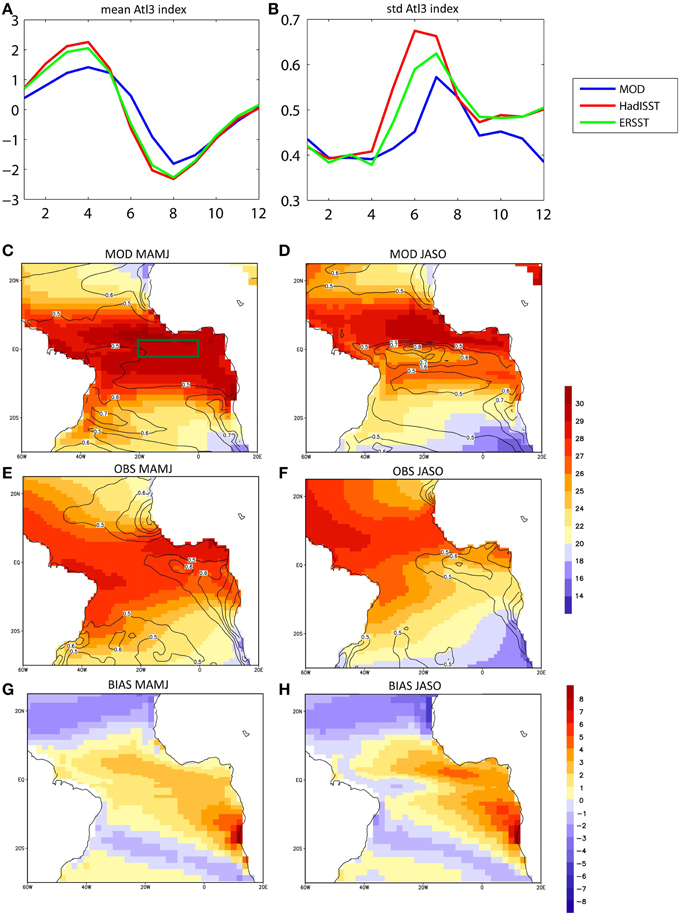
Figure 1. Tropical Atlantic SST bias. Seasonal cycle for the Atl3 index [SST averaged over 20W–0E 3N–3S], (A) mean (minus the long-term mean) and (B) standard deviation for each month for the model (blue) and observations from HadISST dataset (red) and ERSST dataset (green). The IPSL-CM4 model simulates variability over summer season over the eastern equatorial Atlantic. (C) Mean SST (shaded in C) and standard deviation of SST (contours) for MAMJ season for the model. The green square is the Atl3 region (D) same as (C) but for the JASO season. (E,F) same as (C,D) but for the observations (HadISST dataset). (G) SST BIAS (model minus observations, in C) for MAMJ 4-months seasons (H) same as (G) but for JASO.

Here we want to understand the mechanisms behind the Atlantic Niño-like in IPSL-CM4 coupled model. The way the model produces its own Atlantic Niño mode will give more insights in the understanding of the coupled model biases in the inter-annual variability. We will answer the following questions; how is IPSL-CM4, a state-of-the-art coupled model, generating inter-annual TAV? how does the model simulate the main mode of inter-annual variability? What are the processes governing the origin and damping of this mode, in particular the ocean heat fluxes? And finally, are vertical subsurface turbulent processes as important as for the seasonal cycle of the stand- alone ocean model (Peter et al., 2006; Jouanno et al., 2011) and the observations (Foltz et al., 2003; Hummels et al., 2014)? The last interrogation justify by itself the modeling approach we chose, instead of observation derived one, since subsurface mixing observations are far too sparse to allow constructing a reasonably closed heat budget at basin scale.

The article is organized as followed, firstly the model and data used are described with a discussion of the seasonal cycle and the variability in the model, in the results section the mode is described together with the associated heat budget and the main processes are explained. Finally, a discussion and the main conclusions are summarized.

Model and Methods

Although this work is devoted to understand the variability in the coupled model, some observational data has been used throughout the work in order to validate the model (Figure 1–3). For the SST, HadISST (Rayner et al., 2003) and ERSST (Smith and Reynolds, 2003) has been used. For the Mixed Layer Depth (MLD), data from de Boyer Montegut et al. (2004) has been used. Near-surface ocean current estimates come from Ocean Surface Current Analysis (OSCAR) merged satellite dataset (Bonjean and Lagerloef, 2002); surface wind from ERA-Interim reanalysis (Dee et al., 2011) and precipitation CMAP dataset (Xie and Arkin, 1997). In the following section the IPSL-CM4 coupled model is described.

Description of the Model

Fully coupled climate model developed at the Institut Pierre-Simon Laplace, IPSL-CM4 v2 (Marti et al., 2010) has been used. This model is composed of the LMDz4 atmosphere GCM (Hourdin et al., 2006), the OPA8.2 ocean model (Madec et al., 1997), the LIM2 sea-ice model (Fichefet and Maqueda, 1997) and ORCHIDEE 1.9.1 for continental surfaces (Krinner et al., 2005). The coupling between the different parts is done by OASIS (Valcke et al., 2000). The resolution in the atmosphere is 96 × 71 × 19, i.e., 3.75° in longitude, 2.5° in latitude, and 19 vertical levels. The ocean and sea-ice are implemented on the ORCA2 grid (averaged horizontal resolution ~ 2°, refined to 0.5° around the equator, 31 vertical levels). This model was intensively used during the CMIP3. Properties and variability of the large scale oceanic circulation in the model was investigated by Msadek et al. (2010) in the North Atlantic and Marini et al. (2011) in the Southern Ocean. Mignot and Frankignoul (2010) studied the sensitivity of the Thermohaline Circulation to anomalous freshwater input in the Tropics. Representativity of tropical features was investigated in particular in Braconnot et al. (2007) and Lengaigne et al. (2004, 2006), as well as in some multi-model studies (Richter and Xie, 2008; Richter et al., 2014). However, the TAV in this model was not investigated per se.

In addition to the 500 year control simulation, with constant pre-industrial GHG concentration, the heat and salinity budgets in the mixed layer are available over an extra 50 years period. This period, which will be used to investigate TAV, has thus beneficiated from an adjustment of more than 500 years (Marti et al., 2010). Notice that the version of the model used in CMIP5 (IPSL-CM5) does not show an improvement over the tropical Atlantic, therefore we will make use of the available simulations of IPSL-CM4 for understanding processes in the TAV.

Seasonal Cycle in the Model

Figures 1A,B shows the seasonal cycle of the SST over the Atl3 region [20W-0E, 3S-3N]. The observations and the model show in general a good agreement with the timing in the seasonal cycle and its variability. Although the peaks of both, the mean and the variance in the model are delayed by 1 month with respect to the observations, the model seems to be reliable to reproduce the Atlantic Niño seasonality, which is important in terms of tele-connections and impacts (García-Serrano et al., 2008; Losada et al., 2010, 2012). Nevertheless, the model shows an important bias of the annual mean SST over the equatorial region from MAMJ to JASO season (Figures 1C,D).

Correct representation of the timing in the cold tongue evolution is important. Figures 1C–F illustrates the SST in MAMJ and in JASO seasons when the origin and damping of Atlantic Niño occurs respectively. A strongest bias is seen in JASO, and it exceeds 4C, although in the previous MAMJ season the bias is also presented with 2–3C of differences with respect to the observations.

Maximum SST biases are found along the eastern oceanic borders (Figure 1H), in the well-known regions of coastal upwelling. Such biases are very common in coarse resolution coupled models (e.g., Large and Danabasoglu, 2006) or even forced oceanic models (Richter et al., 2012a). Note that the SST bias is maximum during the summer of each hemisphere, which is the season of maximum upwelling (not shown). The SST variability is also biased in the model; maximum variability from MAMJ to JASO occurs over western-central equator, while in the observations the standard deviation shows the cold tongue shape over the eastern-central equator. Strong variability for both, model and observations is found in the Angola/Benguela front.

In summary, Figures 1G,H shows the typical bias in the state-of-the-art models consistent in a dipole pattern of cooling in the north and warming in the south (Grodsky et al., 2012). The northern cooling is related to an excess of wind-induced latent heat loss while the southern warming has been related to both weak winds over the western equator and the related air-sea feedbacks together with reduced alongshore upwelling in the Angola-Benguela region. The later could induce, in turn, an erroneous ocean heat advection (Large and Danabasoglu, 2006; Richter and Xie, 2008; Grodsky et al., 2012; Toniazzo and Woolnough, 2014; Xu et al., 2014).

Figures 2A,B shows the seasonal transition (from MAMJ to JASO) of the mixed layer depth and the surface currents. The modeled mean circulation shows strong westward surface currents at the equator. The strengthening of the North Brazil Current (NBC) along the American coast and the retroflection at 5N in MAMJ-JASO, leading to the eastward North Equatorial Counter Current (NECC), which extends into the Guinea Current in the Gulf of Guinea are satisfyingly simulated. The amplitude of the NECC in the model matches the observed one; however the intensity of NBC is overestimated in the model as well as the westward surface currents at the equator (i.e., −0.4 m/s in the model vs −0.1 m/s in the observations from OSCAR dataset in MAMJ). This bias in the equatorial surface currents can be seen as a northward shift and extension of the South Equatorial Current (SEC), which is present in MAMJ when all the equatorial flow is westward (Figure 2A). The North Equatorial Current (NEC) which has its maximum at 10N-20N is less representative from MAMJ to JASO in the model. Finally, the Equatorial Under-Current (EUC) is also well-simulated by the model with a strengthening from boreal spring to late-summer at 80–120 m (not shown), as it is observed (Bourlès et al., 2002; Arhan et al., 2006; Brandt et al., 2006).

FIGURE 2

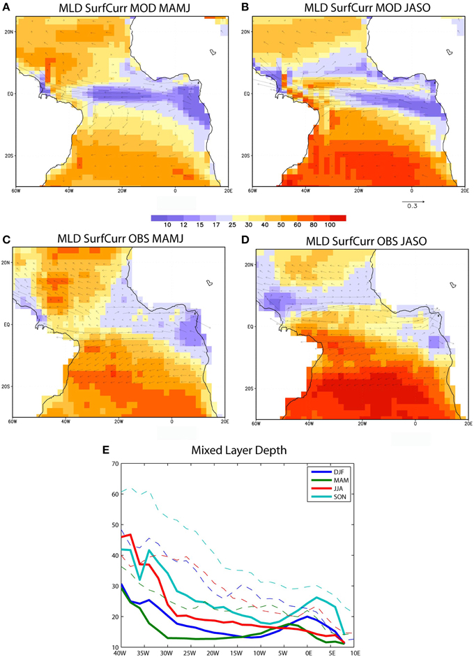
Figure 2. Biases in the TA ocean. (A) Mean Mixed layer depth (shaded in m) and horizontal currents (vectors in m/s) from the model for the MAMJ (B) same as (A) but for JASO 4-months season. (C,D) Same as (A,B) but for the observations. (E) Mixed layer depth in meters for the model (bold lines) and the observations (dashed lines) along the equatorial Atlantic [3N–3S] for the four seasons.

MLD in the model shows an equatorial minimum with a large westward extension in comparison with the observations (Figures 2A,C). A maximum dome in the west equatorial Atlantic at 3N appears in JASO season (Figure 2B) forming a dipole pattern a both side of the equator. However, mixed layer off-equatorial band is quiet well-represented in the model. Additionally, Figure 2 includes the comparison modeled-observed MLD for the four seasons at the equator (Figure 2E). The striking feature is that the model has a reduced MLD all along the year and in particular: (i) in MAM the MLD minimum (~11 m) is found at 30W-20W and in JJA the slope east-west is substantially reduced and the MLD at the west equator is 20 m in the model vs. 40 m in the observations. This westward displacement of the minimum MLD could explain the maximum standard deviation of the SST in Figure 1. Besides, this difference would be important to explain the shape of the variability mode described in the following section.

Figure 3 shows the seasonal transition for the wind stress and precipitation (form MAMJ to JASO). The northward ITCZ-shift is quite well-represented in the model, although the modeled precipitation is located southward compared with the observations especially over West Africa, presumably associated with the warm SST bias over the equatorial Atlantic (Figures 1C,D) and the weaken cross-equatorial surface winds (toward land) in comparison with observations (Figures 3B–D). Next section describes the main Tropical Atlantic variability mode in the model which is related to the rainfall variability over the surrounding land areas.

FIGURE 3

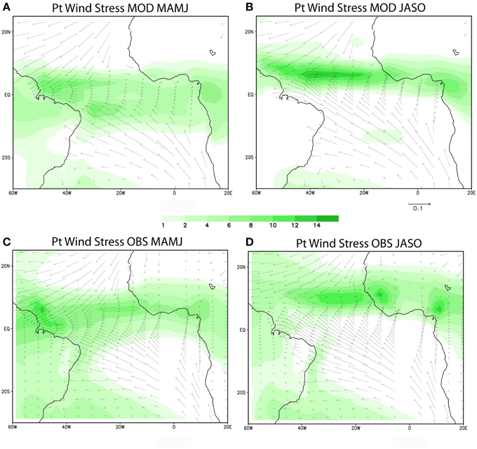
Figure 3. Biases in the TA atmosphere. (A) Precipitation (shaded in kg/day) and wind stress (vectors in N/m2) from the model over Tropical Atlantic for MAMJ (B) same as (A) but for JASO 4-months seasons. (C,D) Same as (A,B) but for the observations.

Methods for Finding the Mode

Previously to determine the leading mode of the equatorial SST inter-annual variability, we have removed the seasonal cycle of the variables and we have applied an inter-annual filter to all the data. To this end, we have subtracted the previous year to the actual year, removing the low-frequency variability and just allowing the inter-annual variability to arise (Stephenson et al., 2000). This is very useful since the equatorial Atlantic has a strong decadal signal which could be mixed with the higher frequencies (see also Figure 4). We are using monthly mean anomalies for all variables.

FIGURE 4

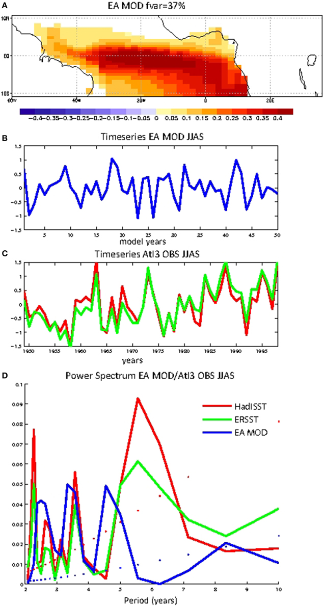
Figure 4. The EA mode: spatial pattern and time-series. (A) spatial pattern of the EA mode (B) Standardized time series for the EA-mode (JJAS mean) (C) Standardized time series for JJAS Atl3 index for the observations, from HadISST dataset (red) and ERSST dataset (green). For the observations the period 1949–2000 has been chosen. (D) Power Spectrum for the time series above-mentioned (50 years). The observations and model have a common peak in [3–4] years band. Multi Tapper method has been used to perform the spectrum and the significance corresponds to 95% confidence level for AR(1) fitting.

The leading co-variability mode between SST over the TA and the rainfall over West Africa is related to a strong ENSO signal (not shown). It shows a warming over the whole tropical basin from MAMJ to JASO associated with anomalous positive rainfall over Sahel region in JJAS (not shown). This mode reflects the excess of tele-connection of El Niño in most of the coupled models (Lloyd et al., 2009) due to atmospheric feedbacks and it is not investigated further here. To this end, we thus have removed the ENSO influence on the Tropical Atlantic following the methodology by Frankignoul and Kestenare (2005). We have reconstructed the global SST with the two leading Principal Components of the tropical Pacific, which is the region [120E-90W, 10S-10N]. The two PC constitute 56% of the total variance. The reconstructed data has been removed from the original data and the tropical SST has been retained.

In order to extract the variability modes, we have computed EOF over the TA monthly mean SST anomalies. Note that the SST-WAM co-variability modes calculated from Extended Maximum Covariance Analysis (EMCA, Polo et al., 2008) do not change substantially from SST EOF modes (not shown). Although the EOF method is simpler than EMCA, it also allows discriminating the variability mode that is phase-locked with the seasonal cycle and in our case, locked within the JJASO season.

Hereafter in the manuscript, the regression and correlation maps are the result of projecting the different model outputs onto the PC time-series of the Equatorial Atlantic (EA) mode, which is associated with the first EOF of TA after pre-processing the data. Ninety percent of confidence level has been used to test the significance of the correlation with a t-test.

Results

Equatorial Atlantic (EA) Mode

The leading mode of SST inter-annual variability over the Tropical Atlantic shows an anomalous warming over the equatorial Atlantic explaining 37% of the variance (Figure 4A). Figures 4B,C shows the time-series of the mode (JJAS mean), together with the Atl3 index for the observations. Seasonality of the EA mode shows a peak in JJASO (not shown).

The power spectra of these time-series are shown in Figure 4D. We have used Multi Tapper Method (Thomson, 1982) to allow more degrees of freedom and significance. The mode highlights maximum of energy in [2–5] year period band, consistent with the observational data (maximum around 2–7 year period band). Peak at 3–4 years is very well-simulated. Next section describes the evolution of the SST pattern and the associated impacts in JJAS precipitation.

Impacts of the EA Mode

Figure 5 shows the regression of the precipitation and SST over the EA time-series for JJAS season. The EA mode is associated with an anomalous southward shift of the rainfall belt during JJAS also related to anomalously warm SSTs covering the whole tropical Atlantic basin (Figure 5, since the EA-mode has a linear nature, the same is true for the opposite case). Warm SST is associated with increased precipitation over the equator, more relevant over the western equatorial Atlantic, suggesting that convection is dislocated westward as an atmospheric response. Rainfall over Brazil and Peru are highly anomalous positive. Associated with the equatorial increase in rainfall, a clear negative anomalous precipitation signal appears over 5-10N in the tropical Atlantic which represents 20% of the precipitation variability of the region in the model. Therefore the onset of West African Monsoon is affected by this EA mode: the evolution of the anomalous negative rainfall shows a latitudinal shift with a maximum over JJAS (not shown), when the rainfall reaches its northernmost position over West Africa. Another significant area of anomalous precipitation is South Africa which could be related to anomalous negative inland flow due to the warming along the Benguela/Namibia coast.

FIGURE 5

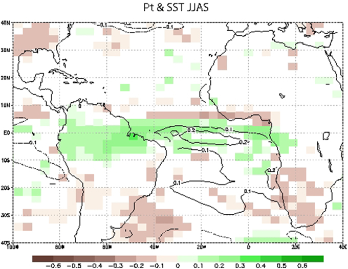
Figure 5. Impacts of the EA mode over TA. Regression map of the anomalous precipitation (shaded in standard deviations) and SST (contour lines in C) onto the EA-mode for JJAS season.

EA Mode Evolution

The evolution of the mode (SST together with the time-derivative of SST) is illustrated in Figure 6 and it is the focus of this study. Since the ENSO effect has been removed, this mode is assumed to be an intrinsic mode of the TA system in the model. The evolution of the mode shows a warming over the equator and the African coast from MJJA to JJAS seasons, with a maximum of about 0.15°C per month over the west equatorial Atlantic in MAMJ and a resulting SST anomaly peaking in size and value in JASO (about 0.2°C over the eastern half equator). Notice that the amplitude of the SST anomalies (0.15°C) corresponds to the filtered data, which is ~0.5°C of the non-filtered data in the model from composites of the highest events (i.e., SST >0.5 in the index). This anomaly represents 0.5°C in the central equatorial Atlantic in JJAS, which is roughly 1 standard deviation in the model (Figure 1). The damping of the anomalies at the equator becomes maximum in JASO season (Figure 6F).

FIGURE 6

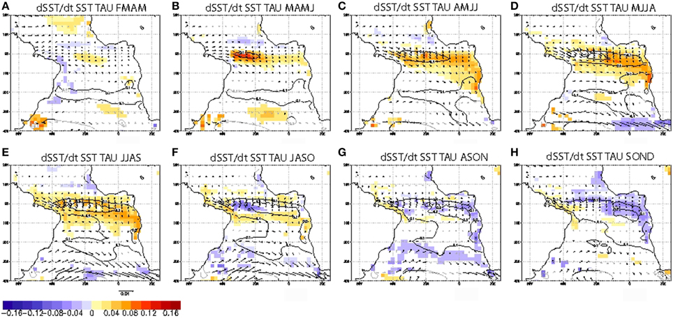
Figure 6. Evolution of the EA mode. Regression map of SST anomalies (contours in C), dSST/dt (shaded in C/month) and wind stress (vectors in N/m2) from FMAM (A) to SOND (H) 4-months seasons onto time-series of the EA mode. Only significant areas have been plotted from a t-test at 90% confidence level.

The equatorial Atlantic warming is associated with a relaxation of the equatorial and trade-winds: southward cross-equatorial anomalous winds are developed as the subtropical winds are also reduced from AMJJ to JASO (Figures 6C–F).

Regarding the similarity of the EA mode from the model and the one found in the observations with the EMCA method (Polo et al., 2008), the model is consistent in amplitude. The amplitude of Atlantic Niño from observations is ~0.4°C over the central equatorial Atlantic in JJAS (see Figure 3 in Polo et al., 2008), which corresponds to half standard deviation.

The main difference between the EA mode in the model and the observational Atlantic Niño is the geographical evolution. Polo et al. (2008) have found the mode starts in MAMJ at the southwest African coast over the upwelling region and the SST anomalies seem to propagate westward and equatorward reaching the whole equatorial band in JASO, consistent with many studies with EOF (i.e., Ruiz-Barradas et al., 2000). The evolution of the SST anomalies in the model is mainly from west equatorial Atlantic to South African coast. The fact that the mode starts ~30W in the simulation could be due to differences in the mean seasonality of the mixed layer depth (Figure 2). The mixed layer in the model results too shallow compared with the observations, especially in the west and thus impacts of surface wind anomalies are integrated by the ocean nearly simultaneously over the whole equatorial Atlantic basin. Despite the differences, the observed warming over the equatorial Atlantic is simulated. Next section investigates this origin from previous winter regressions.

Origin of the EA Mode

Associated with the EA mode, there is anomalous SST around 20S co-varying with the equatorial warming. These SST anomalies are present from FMAM (contour lines in Figure 6A) and are persistent and related to anomalous trades over south Atlantic. In order to understand these preceding anomalies, Figure 7 shows global SST and wind stress projected onto EA mode from previous seasons SOND(-1) to FMAM(0). The subtropical–extra-tropical features related to the mode from previous SOND season are consistent with the observations: SST anomalies over the subtropical South Atlantic in a dipolar-like pattern are presented from previous seasons (SOND), associated with anomalous winds of the South subtropical high pressure system (Figure 7A).

FIGURE 7

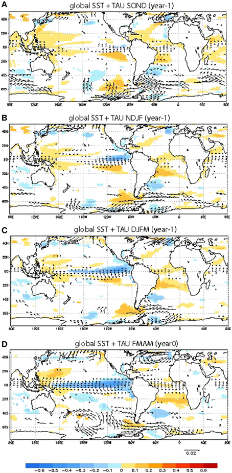
Figure 7. Origin of EA mode. (A) Regression map of the global anomalous SST (shaded in C) and wind stress (vector in N/m2) onto the time-series of the EA mode for the previous SOND (year -1) season. (B) Same as (A) but for NDJF (year -1). (C) same as (A) but for DJFM (year 0). (D) same as (A) but for the FMAM (year 0).

This dipole-like structure in the model develops (Figures 7A–D) increasing both, the wind anomalies and the SST response, and persists almost stationary in the following MAMJ to JASO (contour lines in Figure 6). Tropical/extra-tropical structure over Atlantic in Figure 7A is quite similar to the pattern reported by observational studies (Trzaska et al., 2007; Polo et al., 2008; Nnamchi and Li, 2011). Global pattern in Figure 7D resembles the tele-connection patterns from the Southern Pacific basin via extra-tropical Rossby wave train (Penland and Matrosova, 1998; Barreiro et al., 2004; Huang, 2004) with an associated SST dipolar pattern at both sides of 25S.

Although La Niña pattern is developing the previous NDJF season, the wind anomalies over the south Atlantic seems to appear previously to the Pacific anomalies (Figure 7A), suggesting that the ENSO could enhance anomalous wind structure over south Atlantic via Rossby wave-train but the source in SOND (year-1) rather is intrinsic variability over southern hemisphere in the model (Figure 7). The associated global structure shows an austral hemispheric pattern similar to the Southern Annular mode (Terray, 2011). Although it is difficult to explain why the equatorial SST and the anomalous subtropical SST co-vary from SOND(-1) to ASON (0), the covariance between anomalous equatorial winds and the austral extra-tropical wind (southern 40S) is significant.

In summary, the development of the tropical SST anomalies associated with the EA mode is intrinsic to the tropical Atlantic basin through local feedbacks, but the SST anomalies over the subtropical/extra-tropical basin from the previous seasons (SOND-DJFM) are explained by atmospheric forcing from extra-tropical southern hemisphere and, perhaps, enhanced by ENSO tele-connections.

We will concentrate in understanding how the equatorial SST anomalies are formed and damped. Projections of the surface variables onto EA mode index allow us to understand how the coupled model reproduces an Atlantic Niño-like. The evolution of the EA has a maximum growth in MAMJ and the decay starts in June with a minimum in JASO season (Figure 6). In the next section we will analyze how these SST changes are simulated in the model and what are the associated processes.

The Heat Budget

From the closed heat budget over the mixed layer depth, we have illustrated the components responsible for the formation of the SST anomalies of the EA mode described in Figure 6. Mixed layer temperature equation is decomposed as described by Vialard et al. (2001) and also by Peter et al. (2006). Equation (1) describes the SST tendency integrated over the mixed layer depth h as:

$\begin{array}{ll}\begin{array}{l}{\partial }_{t}T=\underset{a}{\underbrace{-\frac{1}{h}{\displaystyle {\int }_{-h}^{0}u}{\partial }_{x}Tdz-\frac{1}{h}{\displaystyle {\int }_{-h}^{0}v}{\partial }_{y}Tdz-\frac{1}{h}{\displaystyle {\int }_{-h}^0{D}_l}}}\\ \underset{b}{\underbrace{-\frac{1}{h}(T-T_h)(\nabla hu+{\partial }_{z}h)-\frac{1}{h}{[{\kappa }_z{\partial }_{z}T]}_{-h}}}\hfill \\ \underset{c}{\underbrace{-\frac{Q_{rad}(1-F_{-h})+Q_{tur}}{{\rho }_o{C}_{p}h}}}\hfill \end{array}\hfill & \left(1\right)\end{array}$

Integrals represent the quantity integrated over the mixed layer. In Equation (1), T is the temperature in the mixed layer, T_h is the temperature below the mixed layer; u, v and w are the zonal, meridional and vertical currents, respectively, and D_l the lateral diffusion and K_z the vertical mixing coefficient. Q_net is the total net heat flux with the atmosphere and it is divided in radiative Q_rad and turbulent Q_turheat fluxes. F is the function that describes the fraction of shortwave fluxes penetrating the mixed layer, ρ ₀ is the sea water density and C_p is the sea water specific heat capacity coefficient.

The heat budget can be divided into oceanic components and air-sea fluxes forcing (atmospheric components). The total air-sea fluxes forcing is the term (c) on the right hand side and it is the sum of the surface turbulent and radiative heat fluxes. The oceanic part has all the horizontal and vertical terms [a and b on the right hand side of Equation (1)]. Horizontal ocean components (a) are the sum of the horizontal advection plus horizontal diffusion. The vertical terms (b) are the turbulent mixing, vertical advection and an entrainment term computed as the residual following Vialard et al. (2001).

In order to understand the evolution of the EA mode, regression of the terms in the SST tendency equation onto the time-series of the EA mode are analyzed in this section. Note that the regression operator respects the linear partitioning of Equation (1) and that the sum of the regressed terms equals the regressed SST time derivative.

Development of the EA Mode

Figure 8 shows the main components for the MAMJ season, when the warming is maximum in the central equatorial basin. At the equator, there is a large-scale structure which is an intensification of anomalous westerly winds, already seen from previous seasons (i.e., FMAM in Figure 6A). These wind anomalies induce an equatorial positive warming by the oceanic contribution in the mixed layer budget, with a primary maximum in the west and a secondary one in the east (Figure 8A). Noticeably, air-sea fluxes above are negative and principally reduce the ocean dynamics impacts (Figure 8B). Hence the trade reduction is not warming the equator through negative latent heat loss anomalies, as one could have expected, but through its frictional effect on the ocean dynamics. Considering the dependence of the latent heat loss to SST through both, sea level humidity gradient and wind speed, we can conclude that the trade reduction influence on the SST is countered and dominated by the surface humidity increase, itself triggered by the oceanic warming. A similar pattern was found by Sterl and Hazeleger (2003) and Polo et al. (2007) in the observations. Additionally, anomalous positive precipitation and thus anomalous cloud cover over the western-central equatorial Atlantic (especially from AMJJ, not shown) can affect the radiative fluxes by cooling the surface. In summary, air-sea fluxes over the equator merely damp the oceanic warming. In contrast with the climatological seasonal cycle, where air-sea fluxes participate to the cold tongue development through a decrease of their warming effect (not shown), their inter-annual role for the EA mode of variability is only destructive.

FIGURE 8

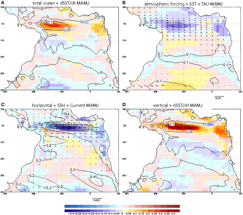
Figure 8. Processes in the development of the EA mode. Heat budget for the mixed layer regressed onto the time-series of the EA mode for the growth season MAMJ. (A) Total Ocean component (shaded in C/month) and total SST tendency (contour, in C/month) (B) Atmospheric component (shaded in C/month), SST (contour in C) and wind stress (vector in N/m2) (C) Horizontal ocean component (shaded in C/month) and SSH (contour in cm) and horizontal surface currents (vectors in m/s) (D) Vertical ocean component (shaded in C/month) and total SST tendency (contour in C/month). The colorbar of purple/red colors are significant areas for the SST tendency at 90% confidence level. Bolded contours and vectors are significant areas.

When searching for the details of the equatorial warming mechanisms, the partitioning of the oceanic contribution point out to the anomaly of vertical fluxes at the base of the mixed layer (Figure 8D), largely associated with turbulent mixing (not shown), which appear as the only cause of the warming, while the horizontal oceanic fluxes contributions are essentially negative. In other words, the net SST anomaly in MAMJ is driven by an upwelling intensity decrease. In coherence with the general behavior of the upwelling systems, the pattern of the vertical component shows a warming also along the African coasts and in particular over both the Ivory Coast and the Angola-Benguela upwelling systems (respectively near 5N-5S, and from the equator down to 20S) reminding the seasonal cold tongue structure (see also Figure 1D). The associated cooling by horizontal oceanic contribution displays a very comparable in amplitude but opposite sign pattern, which anomalous currents are reminiscent in opposite of the seasonal mean South Equatorial Current (see Figure 2A). Considering the net oceanic contribution and the total SST change in MAMJ season, it appears that horizontal dynamics is only able to drive a significant SST anomaly very locally at the Angola-Benguela front, where lie two intense horizontal SST gradient, that is the mean front and an anomalous one (see respectively Figures 1C, 8B).

From MAMJ to JASO, the anomalous equatorial warming on Figure 6 seems to propagate eastward along the equator. Anomalous eastward currents at the Equator in MAMJ (Figure 8C) are wind-driven (vectors in Figure 8B). The SSH anomalies are positive and present along the equatorial and the African coast (contours in Figure 8C), these SSH anomalies suggest that oceanic waves could be interacting by changing the vertical stratification (and thus mixed layer depth h) which would affect the vertical terms (Figure 8D). These vertical terms are the dominated processes in the warming of the equator and African coast associated with the EA mode.

The ocean horizontal component shows a damping pattern eastward of the maximum SST anomaly in MAMJ (Figure 8C), suggesting that horizontal advection (both terms, the mean horizontal currents over the anomalous SST gradient (u_mgradT'), and anomalous currents under mean temperature gradients (u'gradT_m) are responsible for this local cooling (while u'gradT' and u_mgradT_m would warm the surface). Together with horizontal terms, the atmosphere is instantaneously damping the excess of anomalous SST over the region of maximum SST change.

Finally, the Benguela area shows similar behavior although with less intense anomalies than the equatorial band: in FMAM, the wind is reduced over this region, both coastal upwelling cooling and latent heat loss are reduced and act together to warm the surface (not shown). Afterwards (from MAMJ), the SST anomaly becomes important and the atmospheric fluxes turn into a damping term (Figure 8B). Anomalous vertical terms are the main responsible for the warming over the African coast (Figure 8D).

Damping of the EA Mode

The mode terminates with a reduction of the large-scale equatorial wind anomaly (centered on 5S-5N) and a weakening of the Santa Helena pressure system 40S (JASO, Figures 6, 9A,B). In JASO, when the mode enters its vanishing phase, the equatorial SST anomalies are damped between 35W and 10W. Figure 9 shows that it is caused by the oceanic contribution from 35W to 20W, and by the air-sea fluxes effects from 20W to 10W. Whereas there is no other important role for ocean dynamics, the air-sea fluxes also control the damping over almost the whole tropical south Atlantic. As explained above, this suggests that the change in air-sea temperature and humidity gradients are the main components since the wind stress is still anomalously weak (Figure 9B). The damping by vertical humidity surface gradient was a damping mechanism also pointed out by Sterl and Hazeleger (2003) for the tropical-subtropical southern dipole.

FIGURE 9

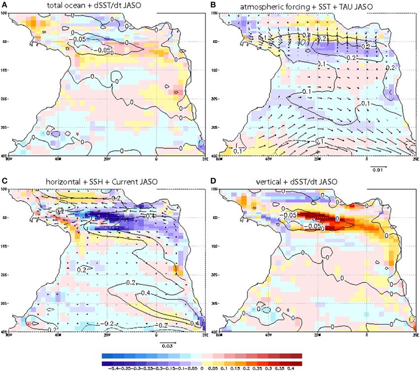
Figure 9. Processes in the damping of the EA mode. Same as Figure 8 but for the decay season JASO.

At the equator, the partitioning of the oceanic terms allows realizing that the total ocean contribution is dominated again by the vertical terms, which warm the eastern half of the change in SST visible on Figure 9A, and cools its western half, helped by the horizontal terms (Figures 9C,D). This reversed sign is probably caused by the reduction of the wind anomaly and the fact that mean vertical currents are now acting in a more stratified ocean. In addition, as in the previous seasons, the important oceanic contribution for the cooling comes from the horizontal component at the eastern of 20W (Figure 9C).

In summary; the ocean is the responsible of the warming over the western part of the equatorial basin and along the African coast by anomalous vertical entrainment while the atmospheric forcing is responsible for warming the South Atlantic region from the previous seasons (not shown) until MAMJ (Figure 8). The atmosphere is damping from the beginning of the SST anomaly formation at the equator and along the African coast.

Discussion and Conclusions

In the IPSL-CM4 coupled model, the leading mode of SST variability is found at the equator and along the African coast in the southern hemisphere. This mode is described and referred here as Equatorial Atlantic (EA) mode. Anomalous westerly winds are associated with an anomalous downwelling pattern along the equator and the African coast, while horizontal terms and the atmosphere are damping the resulting SST anomalies.

It is found that the EA mode is part of the internal TAV in the model, however the EA mode is found to covary with an austral hemispheric mode during previous seasons (from internal extra-tropical atmospheric variability) and possibly enhanced by tele-connection from Pacific La Niña throughout Rossby waves impacting the Sta Helena high pressure system.

Regarding the observations, the mode starts over the Benguela region in boreal spring and then reaches the eastern equator, with a stronger SST signal than the EA mode in the model. The opposite situation occurs in the model; the SST anomalies seem to propagate from the western equator to the African coast. The delayed SST anomalies at the equator have been explained by the different mixed layer depth seasonality in Angola/Benguela region and the eastern equator (Lübbecke et al., 2010). Following the similar reasoning, the reversed propagation in the model (i.e., the SST anomalies start first at the western-central equator and later on at the eastern equator) could be due to the fact that the mixed layer depth seasonality is not well reproduced in the model. Maximum SST variability in MAMJ season is found at 40W-30W at the equator (Figure 1C). This SST variability maximum is also found in the entrainment and vertical diffusion terms (not shown). The fact that the region of maximum variability in SST (and vertical oceanic terms) corresponds to a minimum in MLD in MAM (Figure 2E) suggests that the seasonality of MLD could be tightly linked to the SST changes. Additionally, the model sub-estimates the MLD along the equator but especially west to 20W in MAM season (Figures 2A,C). If the MLD is very shallow, vertical terms will be more effective in changing the temperature, which could result in a positive feedback. Nevertheless, in order to deeply understand how important the MLD bias is for the formation of the SST anomalies and its seasonal evolution, associated with the EA mode, we would need to perform sensitivity experiments and further analysis would be required.

The vertical terms are the major contributor to generate SST anomalies over the equator and along the African coast in IPSL-CM4 (also in other models as CCSM4 see Muñoz et al., 2012). Tropical Atlantic SST variability in models is very sensitive to details in the upper ocean vertical mixing scheme. Hazeleger and Haarsma (2005) investigated the sensitivity of the climate models to the mixing scheme and they found that when the entrainment efficiency is enhanced, the mean and variability over the TA are improved. More work is needed for understanding these processes and the different mixing schemes, which will help to comprehend and reduce biases in coupled models. More investigation could be done using coupled simulation with reduced bias to better discriminate the Atlantic Niño-like mode and the processes involved.

The main results are summarized in this section as follows:

• Even though the IPSL-CM4 model presents a strong mean SST bias over the Atlantic cold-tongue region in JJAS season, the model is able to reproduce the amplitude and the seasonality of the Atlantic Niño inter-annual variability quite well (Figure 1).

• Equatorial Atlantic inter-annual SST variability mode (EA mode) has been identified to occur in the IPSL-CM4 coupled model control experiment. EA mode consists in an anomalous SST over the equatorial Atlantic and African south coast (from MAMJ to JASO) in a cold-tongue shape. This mode is considered as Atlantic Niño-like in the model (Figures 5, 6).

• EA-SST pattern is related to anomalous rainfall in JJAS in a dipole-like structure over the equator and 10N. Anomalous precipitation is found over North Brazil, West Africa and South Africa (Figure 5).

• An anomalous SST dipole over the south West Atlantic (from previous SOND (year-1) to FMAM) occurs to co-vary with equatorial SST anomalies. The SST dipole over south Atlantic in boreal fall-winter preceding the equatorial boreal summer SST anomalies is due to anomalous Sta Helena High pressure system, which seems to be part of the atmospheric extra-tropical internal variability over austral hemisphere and, perhaps, enhanced by the Indo-Pacific tele-connection (Figure 7).

• In the EA mode, the warming (cooling) at the equator and along the African coast is due to anomalous vertical upwelling processes from MAMJ to JASO. Horizontal terms tend to damp the SST anomalies at the east of the maximum SST anomaly. From JASO, the anomalous eastward (westward) currents start to reverse and the vertical ocean starts to cool (warm) at 30W (Figures 8, 9).

• Despite the anomalous wind stress over the equatorial Atlantic, the atmosphere forces the damping of the SST anomalies throughout anomalous turbulent heat fluxes (wind-driven) and radiative heat fluxes (cloud-cover) from MAMJ to JASO.

• EA-SST evolution is found to be weaker and opposite in the model in comparison with the observations: from west equator to the southeast Atlantic. This could be related to the wrong mixed layer depth along the equator in the model which allows the ocean to easily integrate the changes from an anomalous forcing in the western equator. In addition, the model bias of a strong westward surface current at the equator in MAMJ could act to damp in excess the SST anomalies, resulting in decreasing the amplitude of the equatorial SST anomalies of the mode with respect to the observations.

Conflict of Interest Statement

The authors declare that the research was conducted in the absence of any commercial or financial relationships that could be construed as a potential conflict of interest.

Acknowledgments

Irene Polo has been supported by a postdoctoral fellowship funded by the Spanish Government. This work has been also possible thanks to the Spanish projects: Tropical Atlantic Variability and the Climate Shift (TRACS-CGL2009-10285), MOVAC and MUL CLIVAR (CGL2012-38923-C02-01) and the European project PREFACE. PREFACE is the research leading to these results received funding from the EU FP7/2007-2013 under grant agreement no. 603521.

References

Arhan, M., Treguier, A. M., Bourlès, B., and Michel, S. (2006). Diagnosing the annual cycle of the equatorial undercurrent in the Atlantic Ocean from a general circulation model. J. Phys. Oceanogr. 36, 1502–1522. doi: 10.1175/JPO2929.1

CrossRef Full Text | Google Scholar

Barreiro, M., Giannini, A., Chang, P., and Saravanan, R. (2004). On the role of the South Atlantic atmospheric circulation in tropical Atlantic variability. Earth Clim. 147, 143–156. doi: 10.1029/147gm08

CrossRef Full Text | Google Scholar

Bonjean, F., and Lagerloef, G. S. E. (2002). Diagnostic model and analysis of the surface currents in the tropical Pacific Ocean. J. Phys. Oceanogr. 32, 2938–2954. doi: 10.1175/1520-0485(2002)032<2938:DMAAOT>2.0.CO;2

CrossRef Full Text | Google Scholar

Bourlès, B., D'Orgeville, M., Eldin, G., Gouriou, Y., Chuchla, R., DuPenhoat, Y., et al. (2002). On the evolution of the thermocline and subthermocline eastward currents in the equatorial Atlantic. Geophys. Res. Lett. 29, 1785. doi: 10.1029/2002GL015098

CrossRef Full Text | Google Scholar

Braconnot, P., Hourdin, F., Bony, S., Dufresne, J. L., Grandpeix, J., Marti, O., et al. (2007). Impact of different convective cloud schemes on the simulation of the tropical seasonal cycle in a coupled ocean–atmosphere model Clim. Dyn. 29, 501–520. doi: 10.1007/s00382-007-0244-y

CrossRef Full Text | Google Scholar

Brandt, P., Schott, F., Provost, C., Kartavtseff, A., Hormann, V., Bourlès, B., et al. (2006). Circulation in the central equatorial Atlantic: mean and intraseasonal to seasonal variability. Geophys. Res. Lett. 33, L07609. doi: 10.1029/2005GL025498

CrossRef Full Text | Google Scholar

Breugem, W. P., Hazeleger, W., and Haarsma, R. J. (2006). Multimodel study of tropical Atlantic variability and change. Geophys. Res. Lett. 33, J23706. doi: 10.1029/2006GL027831

CrossRef Full Text | Google Scholar

Breugem, W. P., Hazeleger, W., and Haarsma, R. J. (2007). Multimodel Study of Tropical Atlantic Variability and Change. Available online at: http://www.knmi.nl/samenw/tameet/ipcc_ar4_comp

Breugem, W. P., Chang, P., Jang, C. J., Mignot, J., and Hazeleger, W. (2008). Barrier layers and tropical Atlantic SST biases in coupled GCMs. Tellus 60A, 885–897. doi: 10.1111/j.1600-0870.2008.00343.x

CrossRef Full Text | Google Scholar

Carton, J. A., Cao, X., Giese, B. S., and Da Silva, A. M. (1996). Decadal and interannual SST variability in the tropical Atlantic Ocean. J. Phys. Oceanogr. 26, 1165–1175.

PubMed Abstract | Google Scholar

Chang, P. T., Yamagata, P., Schopf, S. K., Behera, J., Carton, W. S., Kessler, G., et al. (2006a). Climate fluctuations of tropical coupled systems – the role of the ocean dynamics. Clim. J. 19, 5122–5174. doi: 10.1175/JCLI3903.1

CrossRef Full Text | Google Scholar

Chang, P., Fang, Y., Saravanan, R., Ji, L., and Seidel, H. (2006b). The cause of the fragile relationship between the Pacific El Niño and the Atlantic Niño. Nature 443, 324–328. doi: 10.1038/nature05053

PubMed Abstract | CrossRef Full Text | Google Scholar

Chang, C. Y., Carton, J. A., Grodsky, S. A., and Nigam, S. (2007). Seasonal climate of the tropical Atlantic sector in the NCAR Community Climate System Model 3: error structure and probable causes of errors. Clim. J. 21, 1053–1070. doi: 10.1175/JCLI4047.1

CrossRef Full Text | Google Scholar

Collins, W. D., Bitz, C. M., Blackmon, M. L., Bonan, G. B., Bretherton, C. S., Carton, J. A., et al. (2006). The Community Climate System Model Version 3 (CCSM3). Clim. J. 19, 2122–2143. doi: 10.1175/JCLI3761.1

CrossRef Full Text | Google Scholar

De Almeida, R. A. F., and Nobre, P. (2012). On the Atlantic cold tongue mode and the role of the Pacific ENSO. Ocean Sci. Discuss. 9, 163–185. doi: 10.5194/osd-9-163-2012

CrossRef Full Text | Google Scholar

de Boyer Montégut, C., Madec, G., Fischer, A. S., Lazar, A., and Iudicone, D. (2004). Mixed layer depth over the global ocean: an examination of profile data and a profile-based climatology. J. Geophys. Res. 109:C12003. doi: 10.1029/2004JC002378

CrossRef Full Text | Google Scholar

Dee, D. P., Uppala, S. M., Simmons, A. J., Berrisford, P., Poli, P., Kobayashi, S., et al. (2011). The ERA-Interim reanalysis: configuration and performance of the data assimilation system. Q. J. R. Meteorol. Soc. 137, 553–597. doi: 10.1002/qj.828

CrossRef Full Text | Google Scholar

Ding, H., Keenlyside, N., Latif, M., Park, W., and Wahl, S. (2015). The impact of mean state errors on equatorial Atlantic interannual variability in a climate model. J. Geophys. Res. Oceans 120, 1133–1151. doi: 10.1002/2014JC010384

CrossRef Full Text | Google Scholar

Fichefet, T., and Maqueda, M. A. M. (1997). Sensitivity of a global sea ice model to the treatment of ice thermodynamics and dynamics. J. Geophys. Res. Oceans 102, 12609–12646. doi: 10.1029/97JC00480

CrossRef Full Text | Google Scholar

Florenchie, P., Lutjeharms, J. R. E., Reason, C. J. C., Masson, S., and Rouault, M. (2003). The source of Benguela Niños in the South Atlantic Ocean. Geophys. Res. Lett. 30, 1505. doi: 10.1029/2003GL017172

CrossRef Full Text | Google Scholar

Foltz, G. R., Grodsky, S. A., Carton, J. A., and McPhaden, M. J. (2003). Seasonal mixed layer heat budget of the tropical Atlantic Ocean. J. Geophys. Res. 108, 3146. doi: 10.1029/2002JC001584

CrossRef Full Text | Google Scholar

Frankignoul, C., and Kestenare, E. (2005). Air–sea interactions in the tropical Atlantic: a view based on lagged rotated maximum covariance analysis. Clim. J. 18, 3874–3890. doi: 10.1175/JCLI3498.1

CrossRef Full Text | Google Scholar

García-Serrano, J., Losada, T., Rodríguez-Fonseca, B., and Polo, I. (2008). Tropical Atlantic variability modes (1979–2002). Part II: time-evolving atmospheric circulation related to SST-forced tropical convection. Clim. J. 21, 6476–6497. doi: 10.1175/2008JCLI2191.1

CrossRef Full Text

Giannini, A., Saravannan, R., and Chang, P. (2003). Oceanic forcing of Sahel rainfall on interannual to interdecadal time scales. Science 302, 1027–1030. doi: 10.1126/science.1089357

PubMed Abstract | CrossRef Full Text | Google Scholar

Grodsky, S. A., Carton, J. A., Nigam, S., and Okumura, Y. (2012). Tropical Atlantic biases in CCSM4. J. Clim. 25, 3684–3701. doi: 10.1175/JCLI-D-11-00315.1

CrossRef Full Text | Google Scholar

Hazeleger, W., and Haarsma, R. J. (2005). Sensitivity of tropical Atlantic climate to mixing in a coupled ocean-atmosphere model. Clim. Dyn. 25, 387–399. doi: 10.1007/s00382-005-0047-y

CrossRef Full Text | Google Scholar

Hourdin, F., Musat, I., Bony, S., Braconnot, P., Codron, F., Dufresne, J. L., et al. (2006). The lmdz4 general circulation model: climate performance and sensitivity to parametrized physics with emphasis on tropical convection. Clim. Dyn. 27, 787–813. doi: 10.1007/s00382-006-0158-0

CrossRef Full Text | Google Scholar

Hu, Z. Z., and Huang, B. (2007). Physical processes associated with the Tropical Atlantic SST gradient during the anomalous evolution in the Southeastern Ocean. Clim. J. 20, 3366–3378. doi: 10.1175/JCLI4189.1

CrossRef Full Text | Google Scholar

Huang, B. (2004). Remotely forced variability in the Tropical Atlantic Ocean. Clim. Dyn. 23, 122–152. doi: 10.1007/s00382-004-0443-8

PubMed Abstract | CrossRef Full Text | Google Scholar

Hummels, R., Dengler, M., Brandt, P., and Schlundt, M. (2014). Diapycnal heat flux and mixed layer heat budget within the Atlantic Cold Tongue. Clim. Dyn. 43, 3179–3199. doi: 10.1007/s00382-014-2339-6

CrossRef Full Text | Google Scholar

Janicot, S., Harzallah, A., Fontaine, B., and Moron, V. (1998). West African monsoon dynamics and eastern equatorial Atlantic and Pacific SST anomalies (1970–1988). Clim. J. 11, 1874–1882. doi: 10.1175/1520-0442-11.8.1874

CrossRef Full Text | Google Scholar

Jouanno, J., Marin, F., du Penhoat, Y., Sheinbaum, J., and Molines, J.-M. (2011). Seasonal heat balance in the upper 100 m of the equatorial Atlantic Ocean. J. Geophys. Res. 116:C09003. doi: 10.1029/2010JC006912

CrossRef Full Text | Google Scholar

Keenlyside, N. S., and Latif, M. (2007). Understanding equatorial Atlantic interannual variability. Clim. J. 20, 131–142. doi: 10.1175/JCLI3992.1

PubMed Abstract | CrossRef Full Text | Google Scholar

Kushnir, Y., Robinson, W. A., Chang, P., and Robertson, A. W. (2006). The physical basis for predicting Atlantic sector seasonal- to-interannual climate variability. Clim. J. 19, 5949–5970. doi: 10.1175/JCLI3943.1

CrossRef Full Text | Google Scholar

Krinner, G., Viovy, N., de Noblet-Ducoudré, N., Ogée, J., Polcher, J., Friedlingstein, P., et al. (2005). A dynamic global vegetation model for studies of the coupled atmosphere-biosphere system. Global Biogeochem. Cycles 19:GB1015. doi: 10.1029/2003GB002199

CrossRef Full Text | Google Scholar

Large, W. G., and Danabasoglu, G. (2006). Attribution and Impacts of Upper Ocean Biases in CCSM3. Clim. J. 19, 2325–2346. doi: 10.1175/JCLI3740.1

CrossRef Full Text | Google Scholar

Latif, M., and Grötzner, A. (2000). On the equatorial Atlantic oscillation and its response to ENSO. Climate Dyn. 16, 213–218. doi: 10.1007/s003820050014

PubMed Abstract | CrossRef Full Text | Google Scholar

Lengaigne, M., Guilyardi, E., Boulanger, J. P., Menkes, C., Delecluse, P., Inness, P., et al. (2004). Triggering of El Nin Þ*o by Westerly wind events in a coupled general circulation model. Clim. Dyn. 23, 601–620. doi: 10.1007/s00382-004-0457-2

CrossRef Full Text | Google Scholar

Lengaigne, M., Boulanger, J. P., Menkes, C., and Spencer, H. (2006). Influence of the seasonal cycle on the termination of El Niño events in a coupled general circulation model. J. Clim. 19, 1850–1868. doi: 10.1175/JCLI3706.1

CrossRef Full Text | Google Scholar

Lloyd, J., Guilyardi, E., Weller, H., and Slingo, J. (2009). The role of atmosphere feedbacks during ENSO in the CMIP3 models. Atmos. Sci. Lett. 10, 170–176 doi: 10.1002/asl.227

CrossRef Full Text | Google Scholar

Losada, T., Rodriguez-Fonseca, B., Janicot, S., Gervois, S., Chauvin, F., and Ruti, P. (2010). A multi-model approach to the Atlantic Equatorial mode: impact on the West African monsoon. Clim. Dyn. 35, 29–43. doi: 10.1007/s00382-009-0625-5

CrossRef Full Text | Google Scholar

Losada, T., Rodriguez-Fonseca, B., and Kucharski, F. (2012). Tropical Influence on the Summer Mediterranean Climate. Atmos. Sci. Lett. 13, 36–42. doi: 10.1002/asl.359

CrossRef Full Text | Google Scholar

Lübbecke, J. F., Böning, C. W., Keenlyside, N. S., and Xie, S.-P. (2010). On the connection between Benguela and equatorial Atlantic Niños and the role of the South Atlantic Anticyclone. J. Geophys. Res. 115, C09015. doi: 10.1029/2009JC005964

CrossRef Full Text | Google Scholar

Lübbecke, J., and McPhaden, M. (2012). On the inconsistent relationship between Pacific and Atlantic Niños. J. Clim. 25, 4294–4303. doi: 10.1175/JCLI-D-11-00553.1

CrossRef Full Text | Google Scholar

Madec, G., Delecluse, P., Imbard, M., and Levy, C. (1997). OPA Version 8.1 Ocean General Circulation Model Reference Manual. Technical Report, LODYC, Paris.

Marini, C., Frankignoul, C., and Mignot, J. (2011). Links between the southern annular mode and the Atlantic meridional overturning circulation in a climate model. J. Clim. 24, 624–640. doi: 10.1175/2010JCLI3576.1

CrossRef Full Text | Google Scholar

Marti, O., Braconnot, P., Bellier, J., Benshila, R., Bony, S., Brockmann, P., et al. (2010). The New IPSL Climate System Model: IPSL-CM4, Note du Pôle de Modélisation n 26, Institut Pierre Simon Laplace des Sciences de l'Environnement Global. Paris: IPSL Global Climate Modeling Group.

Google Scholar

Mechoso, C. R., Robertson, A. W., Barth, N., Davey, M. K., Delecluse, P., Gent, P. R., et al. (1995). The seasonal cycle over the tropical Pacific in coupled ocean-atmosphere general circulation models. Mon. Weather Rev. 123, 2825–2838.

Google Scholar

Mignot, J., and Frankignoul, C. (2010). Local and remote impacts of a tropical Atlantic salinity anomaly. Clim. Dyn. 35, 1133–1147. doi: 10.1007/s00382-009-0621-9

CrossRef Full Text | Google Scholar

Msadek, R., Frankignoul, C., and Li, Z. X. (2010). Mechanisms of the atmospheric response to North Atlantic multidecadal variability: a model study. Clim. Dyn. 36, 1255–1276. doi: 10.1007/s00382-010-0958-0

CrossRef Full Text | Google Scholar

Muñoz, E., Weijer, W., Grodsky, S., Bates, S. C., and Wagner, I. (2012). Mean and Variability of the Tropical Atlantic Ocean in the CCSM4. J. Clim. 25, 4860–4882. doi: 10.1175/JCLI-D-11-00294.1

CrossRef Full Text | Google Scholar

Nnamchi, H. C., and Li, J. (2011). Influence of the South Atlantic Ocean Dipole on West African summer precipitation. Clim. J. 24, 1184–1197. doi: 10.1175/2010JCLI3668.1

CrossRef Full Text | Google Scholar

Namchi, H. C., Li, J., Kang, I. S., and Kucharski, F. (2013). Simulated impacts of the South Atlantic Ocean Dipole on summer precipitation at the Guinea Coast. Clim. Dyn. 4, 677–694 doi: 10.1007/s00382-012-1629-0

CrossRef Full Text

Okumura, Y., and Xie, S. (2004). Interaction of the Atlantic Equatorial cold tongue and the African monsoon. Clim. J. 17, 3589–3602. doi: 10.1175/1520-0442(2004)017<3589:IOTAEC>2.0.CO;2

CrossRef Full Text | Google Scholar

Penland, C., and Matrosova, L. (1998). Prediction of Tropical Atlantic Sea Surface temperatures using linear inverse modeling. Clim. J. 11, 483–496.

Google Scholar

Peter, A.-C., Le He'naff, M., du Penhoat, Y., Menkes, C. E., Menkes, F., Marin, J., et al. (2006). A model study of the seasonal mixed layer heat budget in the equatorial Atlantic. J. Geophys. Res. 111, C06014. doi: 10.1029/2005JC003157

CrossRef Full Text | Google Scholar

Philander, S. G. H. (1990). El Niño, La Niña, and the Southern Oscillation. International Geophysics Series, Vol. 46. San Diego; New York; Berkeley; Boston; London; Sydney; Tokyo; Toronto: Academic Press.

Google Scholar

Polo, I., Rodriguez-Fonseca, B., Garcia-Serrano, J., and Losada, T. (2007). “Interannual West African rainfall-tropical atlantic SST covariability modes during the dry Sahel period (1979-2001),” in Poster Presentation in 2nd International AMMA Conference (Karlsruhe).

Polo, I., Rodriguez-Fonseca, B., Losada, T., and Garcia-Serrano, J. (2008). Tropical Atlantic variability modes (1979-2002). Part I: time-evolving SST modes related to West African rainfall. J. Clim. 21, 6457–6475. doi: 10.1175/2008JCLI2607.1

CrossRef Full Text | Google Scholar

Polo, I., Dong, B. W., and Sutton, R. T. (2013). Changes in tropical Atlantic interannual variability from a substantial weakening of the meridional overturning circulation. Clim. Dyn. 41, 2765–2784. doi: 10.1007/s00382-013-1716-x

CrossRef Full Text | Google Scholar

Rayner, N., Parker, D., Horton, E., Folland, C., Alexander, L., Rowell, D., et al. (2003). Global analyses of sea surface temperature, sea ice, and night marine air temperature since the nineteenth century. J. Geophys. Res. 108, 4407. doi: 10.1029/2002JD002670

CrossRef Full Text | Google Scholar

Richter, I., Behera, S. K., Masumoto, Y., Taguchi, B., Komori, N., and Yamagata, T. (2010). On the triggering of Benguela Niños: remote equatorial versus local influences. Geophys. Res. Lett. 37, L20604. doi: 10.1029/2010GL044461

CrossRef Full Text | Google Scholar

Richter, I., Behera, S. K., Masumoto, Y., Taguchi, B., Sasaki, H., Yamagata, T., et al. (2012b). Multiple causes of interannual sea surface temperature variability in the equatorial Atlantic ocean. Nat. Geosci. 6, 43–47. doi: 10.1038/ngeo1660

CrossRef Full Text | Google Scholar

Richter, I., and Xie, S. P. (2008). On the origin of equatorial Atlantic biases in coupled general circulation models. Clim. Dyn. 31, 587–598. doi: 10.1007/s00382-008-0364-z

CrossRef Full Text | Google Scholar

Richter, I., Xie, S. P., Behera, S. K., Doi, T., and Masumoto, Y. (2014). Equatorial Atlantic variability and its relation to mean state biases in CMIP5. Clim. Dyn. 42, 171–188. doi: 10.1007/s00382-012-1624-5

CrossRef Full Text | Google Scholar

Richter, I., Xie, S.-P., Wittenberg, A. T., and Masumoto, Y. (2012a). Tropical Atlantic biases and their relation to surface wind stress and terrestrial precipitation. Clim. Dyn. 38, 985–1001. doi: 10.1007/s00382-011-1038-9

CrossRef Full Text | Google Scholar

Rodrigues, R. R., Haarsma, R. J., Campos, E. J. D., and Ambrizzi, T. (2011). The impacts of inter-El Niño variability on the Tropical Atlantic and Northeast Brazil climate. Clim. J. 24, 3402–3342. doi: 10.1175/2011JCLI3983.1

CrossRef Full Text | Google Scholar

Rodriguez-Fonseca, B., Janicot, S., Mohino, E., Losada, T., Bader, J., Caminade, C., et al. (2011). Interannual and decadal SST-forced responses of the West African monsoon. Atmos. Sci. Lett. 12, 67–74. doi: 10.1002/asl.308

CrossRef Full Text | Google Scholar

Rodríguez-Fonseca, B., Mohino, E., Mechoso, C. R., Caminade, C., Biasutti, M., Gaetani, M., et al. (2015). Variability and predictability of West African droughts: a review of the role of sea surface temperature anomalies. J. Clim. 28, 4034–4060. doi: 10.1175/JCLI-D-14-00130.1

CrossRef Full Text | Google Scholar

Ruiz-Barradas, A., Carton, J. A., and Nigam, S. (2000). Structure of interannual-to-decadal climate variability in the tropical atlantic sector. Clim. J. 13, 3285–3297. doi: 10.1175/1520-0442(2000)013<3285:SOITDC>2.0.CO;2

PubMed Abstract | CrossRef Full Text | Google Scholar

Smith, T. M., and Reynolds, R. W. (2003). Extended reconstruction of global sea surface temperatures based on COADS data (1854–1997). Clim. J. 16, 1495–1510. doi: 10.1175/1520-0442-16.10.1495

CrossRef Full Text | Google Scholar

Stephenson, D. B., Pavan, V., and Bojariu, R. (2000). Is the North Atlantic oscillation a random walk? Int. J. Climatol. 20, 1–18. doi: 10.1002/joc.1003

CrossRef Full Text | Google Scholar

Sultan, B., Janicot, S., and Diedhiou, A. (2003). The West African Monsoon Dynamics. Part I: documentation of the intraseasonal variability. Clim. J. 16, 3389–3406. doi: 10.1175/1520-0442(2003)016<3389:TWAMDP>2.0.CO;2

CrossRef Full Text | Google Scholar

Sterl, A., and Hazeleger, W. (2003). Coupled variability and air-sea interaction in the South Atlantic Ocean. Clim. Dyn. 21, 559–571. doi: 10.1007/s00382-003-0348-y

CrossRef Full Text | Google Scholar

Terray, P. (2011). Southern Hermisphere extratropical forcing: a new paradigm for El Niño- Southern Oscillation. Clim. Dyn. 36, 2171–2199. doi: 10.1007/s00382-010-0825-z

CrossRef Full Text | Google Scholar

Thomson, D. J. (1982). Spectrum estimation and harmonic analysis. Proc. IEEE 70, 1055–1096. doi: 10.1109/PROC.1982.12433

CrossRef Full Text | Google Scholar

Tokinaga, H., and Xie, S. P. (2011). Weakening of the equatorial Atlantic cold tongue over the past six decades. Nat. Geosci. 4, 222–226. doi: 10.1038/ngeo1078

CrossRef Full Text | Google Scholar

Toniazzo, T., and Woolnough, S. (2014). Development of warm SST errors in the southern tropical Atlantic in CMIP5 decadal hindcasts. Clim. Dyn. 43, 2889–2913. doi: 10.1007/s00382-013-1691-2

CrossRef Full Text | Google Scholar

Trzaska, S., Robertson, A. W., Farrara, J., and Mechoso, C. R. (2007). South Atlantic variability arising from air-sea coupling: local mechanisms and tropical–subtropical interactions. Clim. J. 20, 3345–3365. doi: 10.1175/JCLI4114.1

CrossRef Full Text | Google Scholar

Valcke, S., Terray, L., and Piacentini, A. (2000). The Oasis Coupler User Guide Version 2.4. Technical Report, TR/CMGC/00–10, Paris.

Vizy, E. K., and Cook, K. H. (2001). Mechanisms by which Gulf of Guinea and eastern North Atlantic sea surface temperature anomalies can influence African rainfall. Clim. J. 14, 795–821. doi: 10.1175/1520-0442(2001)014<0795:MBWGOG>2.0.CO;2

CrossRef Full Text | Google Scholar

Vialard, J., Menkes, C., Boulanger, J.-P., Delecluse, P., Guilyardi, E., McPhaden, M. J., et al. (2001). Oceanic mechanisms driving the SST during the 1997–1998 El Nino. J. Phys. Oceanogr. 31, 1649–1675. doi: 10.1029/2001JC000850

CrossRef Full Text

Ward, M. N. (1998). Diagnosis and short-lead time prediction of summer rainfall in tropical North Africa at interannual and multidecadal timescales. Clim. J. 11, 3167–3191.

Google Scholar

Wahl, S., Latif, M., Park, W., and Keenlyside, N. (2011). On the Tropical Atlantic SST warm bias in the Kiel climate model. Clim. Dyn. 36, 891–906 doi: 10.1007/s00382-009-0690-9

CrossRef Full Text | Google Scholar

Xie, S.-P., and Carton, J. A. (2004). “Tropical Atlantic variability: patterns, mechanisms, and impacts,” in Earth Climate: The Ocean-Atmosphere Interaction, Geophysical Monograph Series, Vol. 147, eds C. Wang, S.-P. Xie, and J. A. Carton (Washington, DC: AGU), 121–142.

Google Scholar

Xie, P., and Arkin, P. A. (1997). Global precipitation: a 17-year monthly analysis based on gauge observations, satellite estimates, and numerical model outputs. Bull. Am. Meteorol. Soc. 78, 2539–2558.

Google Scholar

Xu, Z., Li, M., Patricola, C. M., and Chang, P. (2014). Oceanic origin of southeast tropical Atlantic biases. Clim. Dyn. 43, 2915–2930. doi: 10.1007/s00382-013-1901-y

CrossRef Full Text | Google Scholar

Zebiak, S. E. (1993). Air–sea interaction in the equatorial Atlantic region. Clim. J. 6, 1567–1586. doi: 10.1111/j.1600-0870.2008.00343.x

CrossRef Full Text | Google Scholar