Lee Waves on the Boundary-Layer Inversion and Their Dependence on Free-Atmospheric Stability

1. Introduction

Trapped lee waves can be generated in the atmosphere when a mountain perturbs stratified airflow. Unlike other types of mountain waves, trapped waves propagate horizontally (Smith, 1979): their phase lines are vertical and multiple wave crests can extend over several hundreds of kilometers downstream of an obstacle. If the atmosphere contains sufficient moisture, clouds may form at the wave crests (Houze, 2014) and give rise to a characteristic stripe pattern, frequently observed in satellite images close to mountainous areas, e.g., the Alps (Doyle et al., 2002), Pyrenees (Georgelin and Lott, 2001), Rocky Mountains (Ralph et al., 1997), and Pennines (Vosper et al., 2012).

Trapped lee waves can be expected to develop if the atmospheric structure promotes vertical trapping and horizontal propagation of wave energy. This occurs either when the Scorer parameter $l^2=\frac{N^2}{U^2}-\frac{1}{U}\frac{d^{2}U}{d{z}^2}$ (where N is the buoyancy frequency and U the wind speed) decreases with height (Scorer, 1949), or along a density discontinuity, e.g., a temperature inversion. Both of these conditions lead to horizontal propagation of wave energy. In the former case, this happens through wave reflection and superposition in a wave duct; in the latter case, through adjustment to horizontal pressure gradients generated by the deflection of the discontinuity. These two mechanisms have traditionally been regarded as distinct and unrelated. The former has often been highlighted as the primary mechanism that gives rise to trapped lee waves in the atmosphere (e.g., Durran, 1986b; Wurtele et al., 1996; Teixeira, 2014), while the latter has been emphasized mostly in oceanographic investigations, for instance to explain surface water waves and the phenomenon of dead water (Gill, 1982). In what follows, we refer to the theories that describe these two processes, respectively, as the internal wave theory and the interfacial wave theory¹.

The internal gravity wave framework, where density is assumed to be a continuous function of height, was used by Scorer (1949) to develop a theory for lee waves in a two-layer atmosphere. Scorer attributed the origin of trapped lee waves to a discontinuity in the parameter l², defined above. For l higher in the lower layer, horizontal wave propagation results from the linear superposition of two internal gravity wave modes, an upward-propagating one, excited by the flow over the mountain, and a downward-propagating one arising through wave reflection at the interface between the two layers.

Scorer (1949) also applied interfacial wave theory to atmospheric lee waves that form on a density discontinuity. However, that part of his work has received only little attention. After Scorer's, probably the first study explicitly addressing interfacial lee waves was made by Vosper (2004). Seeking for the most favorable environment for the formation of lee-wave rotors and low-level hydraulic jumps, Vosper (2004) analyzed the conditions that lead to wave trapping at a boundary-layer inversion underneath a continuously-stratified atmosphere. For such a density profile, interfacial waves along the inversion and vertically-propagating wave modes in the free atmosphere may occur at the same time. Teixeira et al. (2013) investigated the magnitude of wave drag, generated by both interfacial and vertically propagating waves in this scenario, and determined the state of maximum total drag. Although these two studies shed light on important aspects of interfacial lee waves, an assessment of how their wavelength (the most striking and immediate feature of the phenomenon, as visible in satellite images) depends on the environmental conditions in the free atmosphere still seems to be lacking. Therefore, the first objective of this paper is to improve the current understanding of the impact of the stratified free atmosphere on the dynamics—and the wavelength in particular—of interfacial lee waves that form at the boundary-layer inversion.

A related theme is the applicability of hydraulic analogies to the quantitative description of layered atmospheric flows. The possibility of a hydraulic-type response in two-layer mountain flow (with discontinuous l²) was first demonstrated by Durran (1986a), who suggested that transition to supercritical flow at the top of a mountain is an effective mechanism to generate downslope windstorms. The applicability of hydraulic theory, however, depends on stratification in the free atmosphere, which affects the validity of two of the basic assumptions, namely: (i) the presence of a passive upper layer, i.e., one that causes no horizontal pressure gradient force on the lower layer (Jiang and Smith, 2001), and (ii) hydrostatic conditions, which imply the validity of the shallow-water (long-wave) approximation. Relationships between free-atmospheric stratification and the validity of the passive layer assumption have been explored by Jiang (2014). A similar study focusing on the long-wave approximation, however, still seems to be lacking. Hence, the second aim of this study is to explain how static stability in the free atmosphere affects the accuracy of the shallow-water theory when applied to low-level flow below an inversion.

We begin by reviewing the existing theories of trapped lee waves in Section 2. By taking representative values of free-atmospheric stability and inversion strength from an observed lee-wave event (Section 3), we describe how different linear analytical models lead to different estimates of lee wavelength for the same conditions (Section 4). Recognizing the important role played by free-atmospheric stratification, in Section 5 we discuss its impact on lee wavelength and on the applicability of shallow-water theory. Conclusions are drawn in Section 6.

2. Review of Lee Wave Theories

As briefly discussed in the Introduction, the simplest models of trapped lee waves consider uniform wind speed and a vertical discontinuity, either in the Scorer parameter l or in potential temperature θ. Such discontinuities are responsible for different wave-trapping mechanisms, which may co-exist for a vertical potential temperature profile like the one shown in Figure 1. The defining parameters of this type of flow are the buoyancy frequencies in the lower and upper layer (N₁ and N₂ respectively), the potential temperature jump across the interface (Δθ), the potential temperature at the ground (θ₀) and the height of the lower layer (h₁).

FIGURE 1

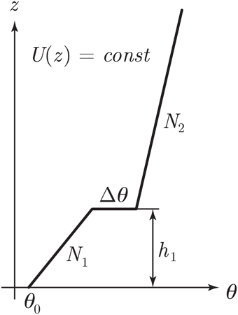
Figure 1. Vertical potential temperature (θ) profile of a generic two-layer flow with a density interface. The wind profile U(z) is assumed to be constant with height (not shown).

In general, the dynamics of wave propagation can be concisely described by a frequency dispersion relationship (FDR), i.e., a relation between the intrinsic frequency of the wave, Ω, and the wavenumber, k. For simplicity, we focus on flows with uniform background wind speed U. The Scorer parameter simplifies to $l^2=\frac{N^2}{U^2}$ in this case. Since lee waves are typically stationary, we consider only wave modes that do not move in a reference frame attached to the mountain, thus Ω∕k − U = 0. All wave modes k that satisfy this relation are stationary with respect to the mountain.

For the stability profile in Figure 1, the FDR of trapped lee waves can be derived by assuming that wavelike solutions to the governing equations exist in each of the two layers. The derivation, presented in the Appendix, leads to:

$\begin{array}{ll}{U}^2=\frac{g\prime }{i{m}_1\text{coth}\left(i{m}_1{h}_1\right)-i{m}_2}.& (1)\end{array}$

Here, h₁ is the finite thickness of the lower layer (the upper one being instead infinitely deep), $g\prime =g·\Delta \theta ∕{\theta }_0$ is the reduced gravity at the interface and $m_{1,2}={(l_{1,2}^2-k^2)}^{1∕2}$ are the vertical wave-numbers in the lower (subscript 1) and in the upper layer (subscript 2) respectively.

Equation (1) summarizes the behavior of four wave types that may occur in common atmospheric conditions:

– Internal interface waves, developing at a density discontinuity between two neutrally stratified fluid layers (Δθ ≠ 0, N_{1, 2} = 0).

– Free interface waves, propagating along a density discontinuity between a lower neutral layer and an upper stably stratified passive layer (Δθ ≠ 0, N₁ = 0, m₂ = 0).

– Forced interface waves, similar to the previous case, but with an upper stably stratified active layer (Δθ ≠ 0, N₁ = 0, m₂ ≠ 0).

– Resonant trapped waves, developing at a discontinuity in the Scorer parameter (Δθ = 0, N₁ > N₂ > 0).

These wave types, and the conditions under which they may form, are described in greater detail in what follows.

2.1. Internal Interface Waves

If both fluid layers are neutrally stratified, wave energy is concentrated at the density discontinuity between them, because all wave modes are evanescent below and above it ($m_{1,2}^2<0$). If the source of the wave energy is at the surface, as is the case with mountain waves, higher altitudes of the interface will result in lower lee wave amplitudes. This happens because evanescent wave modes decay with increasing distance from the wave source. Assuming N_{1, 2} = 0 in Equation (1), the FDR of stationary interfacial waves becomes (Turner, 1973):

$\begin{array}{ll}{U}^2=\frac{g\prime }{k\text{coth}(k{h}_1)+k}.& (2)\end{array}$

The coth(kh₁) term in Equation (2) is non-periodic in k, because the argument is a real number. Thus, only a single stationary wave mode can exist on the density discontinuity. The FDR in Equation (2) describes interfacial waves at internal boundaries with a non-passive upper layer, which is the case for relatively short wave modes ($\partial p_2^{\prime }∕\partial x\ne 0$ if k > 0, $p_2^{\prime }$ being the pressure perturbation in the upper layer; see e.g., Nappo, 2012).

Equation (2) is well-known in its long-wave approximation form, where the condition kh₁ ≪ 1 leads to the non-dispersive FDR:

$\begin{array}{ll}U={(g\prime h_1)}^{1∕2}.& (3)\end{array}$

Another limiting case of Equation (2), that gained less attention in meteorological literature, can be derived by adopting the short-wave approximation, kh₁ ≫ 1:

$\begin{array}{ll}U={(g\prime ∕2k)}^{1∕2}.& (4)\end{array}$

Unlike Equation (3), Equation (4) retains the dispersive character of Equation (2) and can be solved for k to estimate the wavelength of a stationary internal interface wave. The FDRs in Equations (3) and (4) are similar to those of shallow- and deep-water external waves, which correspond to the limit g′ → g. However, since Equations (3) and (4) apply to flows where the upper layer has non-negligible density, they still describe internal interface wave modes.

2.2. Free Interface Waves

Interfaces that are not subject to stress exerted by the upper fluid are referred to as free surfaces. The passive layer assumption, $\partial p_2^{\prime }∕\partial x=0$, applies in this case. Special cases of free surfaces are those where the density difference between the two fluid layers is very large, e.g., between water and air. The corresponding theory was developed by Airy (1841), who firstly derived the universal FDR of (external) water waves (Craik, 2004):

$\begin{array}{ll}{U}^2=\frac{g}{k\text{coth}(k{h}_1)}.& (5)\end{array}$

This equation is not generally valid in atmospheric flows, which are typically characterized by very small density discontinuities. However, even in the atmosphere it is possible for a density discontinuity (e.g., the capping inversion of the convective boundary layer) to act as a free surface. This is the case if N₁ = 0 and m₂ = 0. The second constraint means that any internal gravity wave mode in the stably-stratified upper layer must have vertical phase lines at the interface. In this case, Equation (1) becomes:

$\begin{array}{ll}{U}^2=\frac{g\prime }{k\text{coth}(k{h}_1)}.& (6)\end{array}$

Although this wave type occurs in the interior of a fluid, the interface behaves as a free surface. The upper layer is passive because of the condition m₂ = 0, which implies that wave perturbations in the pressure field, and consequently the horizontal pressure gradient, must vanish therein, as can be demonstrated from the polarization relationships of internal gravity waves (see, e.g., Nappo, 2012). The same applies to wave perturbations in the horizontal wind speed. The FDR of these (internal) free interface waves is similar to that of (external) water waves in Equation (5), except for reduced gravity g′ instead of g.

2.3. Forced Interface Waves

Interfacial waves conform to Equation (6) only when their horizontal wavenumber is equal to the Scorer parameter in the atmosphere aloft (in fact, m₂ = 0 implies k = l₂). In general, however, k ≠ l₂. In this case the upper layer is not passive, i.e., waves propagating along the interface are subject to forcing from internal waves above. The FDR describing these (internal) forced interface waves is obtained from Equation (1) by requiring N₁ = 0 and maintaining a wave-permitting layer with N₂ > 0 aloft (Scorer, 1997):

$\begin{array}{ll}{U}^2=\frac{g\prime }{k\text{coth}\left(k{h}_1\right)+\sqrt{k^2-l_2^2}}.& (7)\end{array}$

Equation (7) is the general form of the FDR considered by Vosper (2004), which is the corresponding short-wavelength (kh₁ ≫ 1) approximation. All wave modes satisfying $k^2<l_2^2$ ($m_2^2>0$) can propagate into the upper stratified layer, hence they are not trapped at the interface. Consequently, the condition $k^2=l_2^2$ defines a critical wavenumber, i.e., the lowest wavenumber (longest wavelength) for which wave trapping is possible. This condition transforms Equation (7) into Equation (6), i.e., into the special case of a free interfacial wave (Section 2.2), and generates the maximum total wave drag (Teixeira et al., 2013).

Equation (7) shows that, given N₂ and U, the critical wavenumber depends on the inversion strength Δθ (through g′) and on the lower layer depth h₁. Critical values for Δθ and h₁ can be determined inserting k = l₂ = N₂ ∕ U into Equation (7). Solving for Δθ or h₁ then gives:

$\begin{array}{llll}\hfill \Delta {\theta }_{crit}& =\frac{N_{2}U{\theta }_0}{g}·\text{coth}\left(\frac{N_2{h}_1}{U}\right)& & (8)\end{array}$

$\begin{array}{llll}\hfill h_{1crit}& =\frac{U}{N_2}·\text{acoth}\left(\frac{g\prime }{N_{2}U}\right)& & (9)\end{array}$

Inversions with strength Δθ ≥ Δθ_crit, or located at height h₁ ≥ h_1crit, cause wave trapping because they make stationary waves become evanescent in the layer aloft.

2.4. Resonant Trapped Waves (g′ = 0)

Setting g′ = 0 (that is, Δθ = 0) in Equation (1) simplifies it to (Scorer, 1949):

$\begin{array}{ll}\text{coth}\left(i{m}_1{h}_1\right)=\sqrt{\frac{l_2^2-k^2}{l_1^2-k^2}}.& (10)\end{array}$

Therefore, wave trapping occurs even in absence of a density discontinuity if a wave mode k that satisfies Equation (10) exists. Scorer (1949) showed that this is the case if

$\begin{array}{lll}\hfill l_1^2>k^2>l_2^2& & (11)\end{array}$

$\begin{array}{lll}\hfill l_1^2-l_2^2>\frac{{\pi }^2}{4h_1^2}.& & (12)\end{array}$

In these conditions, an internal gravity wave mode that propagates vertically in the lower layer is reflected at the discontinuity of l², above which it becomes evanescent. The superposition of the reflected and primary mode generates a stationary wave with vertical phase lines, trapped in the layer below the interface. We refer to this wave type as a resonant trapped wave. In contrast to the FDRs for interfacial waves [Equations (2), (6), and (7)], the argument of the cotangent function in Equation (10) is imaginary. Since the roots of coth(im₁h₁) are periodic, multiple resonant modes may exist. The amplitude of these modes depends essentially on the interface height and on the mountain shape. In general, the mode with the wavelength closest to the mountain half-width L is dominant.

2.5. Bridging the Theories of Interfacial and Resonant Trapped Lee Waves

Wave propagation in stratified fluids with a more complex vertical structure, i.e., with more than two layers, has been studied with analytical models in the past. For instance, Baines (1995, p. 189) formulated a non-hydrostatic three-layer model, that can be used to estimate the horizontal wavenumber of a lee wave trapped along a finite-thickness inversion. In this case, the wavenumber k satisfies the following FDR:

$\begin{array}{cc}\begin{array}{l}\left[\text{tan}(m_1{h}_1)-\frac{i{m}_1}{m_2}\right]\left(m_2-m_3\right)=e^{-2i{m}_{2}d}\left[\text{tan}(m_1{h}_1)+\frac{i{m}_1}{m_2}\right]\\ \left(m_2+m_3\right).\end{array}& \left(13\right)\end{array}$

Here, subscripts j = 1, 2, 3 denote the fluid layers, numbered from below; $m_j={\left(N_j^2∕U^2-k^2\right)}^{1∕2}$ is the vertical wavenumber in each of the layers; h₁ is the thickness of the lowest layer and d that of the middle one (the inversion layer). The third layer represents the free atmosphere, which is assumed to be infinitely deep. Equation (13) is transcendental, because it has no closed-form solutions for k. Moreover, it remains transcendental even after adopting the long- (kh₁ ≪ 1) or short-wave (kh₁ ≫ 1) approximations, in contrast to the two-layer models introduced in Sections 2.1–2.3 above.

In the strict limit of the middle layer depth being zero (d = 0), the inversion disappears and the FDR in Equation (13) approaches the FDR for resonant waves (Equation 10). This is to be expected as the Baines (1995) model assumes a continuous density profile.

For small but finite values of the inversion depth and the finite value of Δθ across the inversion, one would expect the solution of Equation (13) to converge to that of the most general two-layer model (Equation 1), assuming that all other parameters are the same. We show this to be true in the following section by numerically solving Equation (13) for a specific case (cf. Figure 3).

3. Waves Along The Boundary-layer Inversion

The typical thermal structure of the convective boundary layer (N₁ ≈ 0, N₂ > 0, Δθ > 0) is such that it supports forced interface waves (Section 2.3). Since similar conditions are often present above ocean surfaces, or at daytime during the warm season over land, it is likely that wave trapping at the boundary layer inversion is a common mechanism for lee waves.

To confirm this hypothesis, we study a lee wave event that occurred on 24 December 2013 downstream of the Desertas islands. These islands are part of the Madeira archipelago, located in the subtropical Atlantic ~800 km south-west of mainland Portugal. The Desertas are elongated in the N-S direction and reach an altitude of 300 m MSL. Sufficient data is available in this area to estimate the wavelength (from high-resolution satellite images) and the vertical structure of the atmosphere (from operational radiosonde observations in Funchal, Madeira's capital).

The satellite image in Figure 2A shows a characteristic cloud-stripe pattern, generated by a trapped wave leeward of the Desertas islands. The lee wave train is not visibly influenced by the prominent wake of Madeira (Grubišić et al., 2015) and extends over a distance of 40 km with approximately nine wave crests, hence λ ≈ 4.4 km.

FIGURE 2

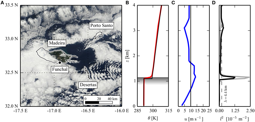
Figure 2. (A) MODIS Terra visible satellite image on 24 December 2013, showing signature of trapped lee waves downwind of the Desertas islands in the Madeira archipelago. Coastlines are shown with solid white-black contours. The location of the sounding site (Funchal) is marked with a black dot. Flow is from left to right. Satellite image from NASA Earthdata and SRTM topography data from Jarvis et al. (2008). (B–D) Funchal operational sounding at 1200 UTC 24 December 2013. The panels show vertical profiles of (B) potential temperature, (C) wind speed projected in lee wave direction and (D) Scorer parameter l² ≈ [N∕U(z)]² (black), l² ≈ [N∕U]² with U = 10 m s⁻¹(gray) and observed wavenumber k² (dashed). The solid black lines in (B,C) show the approximated idealized sounding that defines the parameters listed in Table 1. Gray shaded areas in (B) indicate regions where relative humidity RH > 90%.

The vertical structure of the atmosphere during this event, as measured in nearby Funchal, is shown in Figure 2B. It consists of a neutrally stratified lower layer (N₁ = 0) with θ₀ = 291 K, a boundary-layer inversion with Δθ = 8 K at h₁ = 1100 m and a continuously stratified free atmosphere with N₂ = 0.010 s⁻¹ aloft. The flow is westerly with almost no directional shear. A representative value of U = 10 m s⁻¹ for the wind speed is determined from the wind profile in Figure 2C as the average in the layer below z = 2h₁. The altitude of the inversion coincides with the layer of largest relative humidity (gray shading, RH = 97% at h₁ = 1100 m), implying that the cloud pattern in Figure 2A likely corresponds to an interfacial wave. Further evidence for the interfacial wave character of the disturbance is provided by the Scorer parameter profiles in Figure 2D. The observed wave mode (dashed black) is evanescent (k² > l²) below and above the inversion, indicating that the disturbance can only propagate along it. The flow configuration determined from Figure 2B is similar to that causing forced interfacial waves (Section 2.3).

Given its small thickness, the inversion layer can be approximated as a density discontinuity. This is supported by a comparison between the solutions of Equation (1), which is derived from the discontinuous two-layer model, and Equation (13), which is derived from the continuous three-layer model introduced in Section 2.5. Both equations are solved numerically for λ = 2π∕k, imposing the sounding parameters presented above and letting d in the three-layer model vary in the range between 0 and 1000 m. The results in Figure 3 reveal a difference of ~5% in the wavelength estimates for d = 150 m, which corresponds to the observed profile. This level of accuracy is sufficient for our needs. Hence, from now on, we only consider two-layer models, with the benefit that an analytical solution for k is possible (if the short-wave approximation is adopted).

FIGURE 3

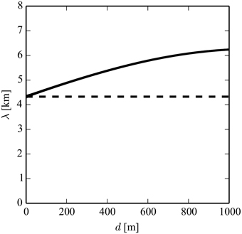
Figure 3. Comparison of the wavelength λ estimated from the FDR of forced interfacial waves (Equation 7, dashed) and from the Baines (1995) three-layer model (Equation 13, solid).

In what follows, we use observations from the Desertas islands to provide numerical values for the parameters of the linear models described in Section 2, and thereby explore the impact of free-atmospheric stratification on interfacial waves.

4. Linear Theory Results

Our two-dimensional, two-layer linear model is described in detail in the Appendix. We solve it for the perturbation velocity fields u′(x, z) and w′(x, z) as a function of the flow profile (N₁, N₂, U, Δθ, h₁) and the topography h₀(x). The latter is specified with a cosine function, in analogy to Vosper (2004):

$h_0(x)=\{\begin{array}{ll}H/2+H/2·\text{cos}\left[\frac{\pi }{L}(x-x_0)\right]\hfill & \text{if}{x}_{\text{0}}-L<x<x_{\text{0}}+L\hfill \\ 0\hfill & \text{elsewhere}\hfill \end{array}$

Here, H = 300 m denotes the mountain height and L = 2 km its half-width, while x₀ is the location of the mountain top. The model parameters (N₁, N₂, U, Δθ, h₁) are estimated from the idealized sounding in Figures 2B,C and are listed in Table 1.

TABLE 1

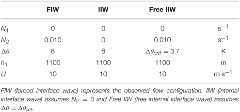
Table 1. Flow parameters determined from the sounding in Figure 2.

Figure 4 shows the wave field predicted by linear theory in two-layer flow over the mountain for two combinations of parameters, one reflecting the observations (N₂ = 0.010 s⁻¹, Figures 4A,D) and the other disregarding stratification in the free atmosphere (N₂ = 0, Figures 4B,E). For completeness, in Figures 4C,F we also show the wave field for the special case Δθ = Δθ_crit, i.e., when the interface acts as a free surface (Section 2.2).

FIGURE 4

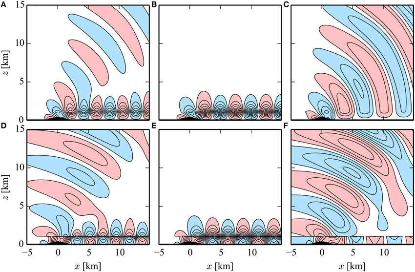
Figure 4. Wave perturbations $w_{1,2}^{\prime }$ (top) and $u_{1,2}^{\prime }$ (bottom) determined from linear model solutions (Equations A2 and A3). Model parameters are listed in Table 1 and correspond respectively to: (A–D) forced interface waves; (B–E) internal interface waves; (C–F) free interface waves. Red and blue shading denote respectively positive and negative areas. The contour interval is 0.5 m s⁻¹.

Two wave branches are evident in the wave perturbations u′ and w′ in Figures 4A,D: a vertically propagating internal gravity wave and an interfacial wave. The mountain wave branch consists of those wave modes that can propagate into the continuously stratified upper layer ($k^2<l_2^2$). The interfacial disturbance, in contrast, consists of a single stationary wave mode, described by Equation (7). The wavelength of this stationary mode (λ = 4.2 km) is close to the observations (λ = 4.4 km) in the satellite image in Figure 2A. Both u′ and w′ reach their maximum amplitude at the interface height. While w′ is continuous across the interface, u′ is discontinuous and changes sign as a consequence of the incompressibility constraint.

The wave structure in flow with a neutral upper layer in Figures 4B,E is different. As expected, the wave branch in the upper layer vanishes due to the absence of stratification in the free atmosphere. The wavelength of the disturbance (λ = 5.0 km), determined from Equation (2), increases slightly (by 19%) compared to that in Figure 4A. This suggests that free-atmospheric stratification does not impact the lee wavelength significantly for the case examined in this paper. This aspect is discussed in more detail in Section 5.

In the special case where Δθ = Δθ_crit, the wave field consists of a free interfacial disturbance with a wavelength of λ = 2π∕l₂ (Figures 4C,F). In this case, the perturbations u′ necessarily vanish right above the inversion, as discussed in Section 2.2. In fact, u′ is confined entirely in the layer below the inversion in Figure 4F, similarly to what happens in water waves. The vertical wind speed w′, in contrast to u′, is continuous across the interface. In this case, λ = 6.3 km.

Given the relatively good agreement between observations and linear model results in the Desertas lee-wave case, we use linear theory to explore the dependence of the lee wavelength (λ = 2π∕k) on the flow parameters (Δθ, h₁, N₂, U). We impose N₁ = 0, because convective boundary layers are typically neutrally stratified.

We proceed by solving the FDRs of internal interface waves (IIW, Equation 2) and of forced interface waves (FIW, Equation 7), varying systematically one of the four parameters mentioned above while keeping all others unchanged. We consider the IIW (N₂ = 0) and FIW (N₂ ≠ 0) flow models because the difference between their solutions allows us to appreciate the impact of free-atmospheric stratification on the lee wavelength. The lee wavelengths, λ_IIW and λ_FIW, are obtained numerically, because the FDRs are transcendental and cannot be solved analytically.

The results of this elaboration are shown in the four panels of Figure 5, which consider Δθ ∈ [0, 15] K, h₁ ∈ [0, 5000] m, N₂ ∈ [0, 0.03] s⁻¹, and U ∈ [0, 15] m s⁻¹; λ_IIW and λ_FIW are shown in all panels as dashed and solid lines respectively. White dots in Figures 5A,B mark the critical values Δθ_crit (Equation 8) and h_1crit (Equation 9). The behavior of λ_IIW and λ_FIW is generally similar: they increase with increasing wind speed U, while they decrease with increasing Δθ and h₁. While λ_FIW decreases with N₂, λ_IIW is inherently independent of it, because N₂ = 0 in the IIW model.

FIGURE 5

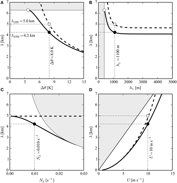
Figure 5. Dependence of the lee wavelength λ on: (A) inversion strength, Δθ; (B) inversion height, h₁; (C) free-atmospheric stratification, N₂; and (D) wind speed, U. Solid and dashed lines correspond respectively to λ_FIW and λ_IIW. Black dots represent the wavelength estimated from the observed flow profile (see Figure 2); gray dots indicate the corresponding wavelength when N₂ = 0; and white dots mark the critical values Δθ_crit and h_1crit at the corresponding wavelength λ = 2πU∕N₂. Shaded areas indicate the propagating regime in the upper layer, i.e., where wave trapping on the interface is not possible.

Since N₂ is the only parameter that differs between the IIW (N₂ = 0) and the FIW model (N₂ ≠ 0), large differences between λ_IIW and λ_FIW indicate that interfacial waves are heavily affected by the free-atmospheric stratification. This is the case for: weak inversions (Figure 5A, maximum deviation 38%), high wind speeds (Figure 5D, maximum deviation 27%) and for strong stratification (Figure 5C, maximum deviation 117%). Conversely, λ_IIW and λ_FIW both become independent of the layer height h₁ for values beyond h₁ > 1100 m (Figure 5B). This indicates that the short-wave (or deep-water) approximation is valid for the Desertas lee-wave case examined (the FDR is then independent of h₁, see Equation 4).

5. Discussion

The results described in Section 4 suggest that stratification in the free atmosphere can indeed have a significant influence on the length of interfacial trapped lee waves. In Section 5.1 below, we determine this impact more precisely after simplifying the FDRs of the FIW and IIW models with the short-wave approximation.

Besides controlling lee wavelength, a continuously-stratified free atmosphere limits the range of possible trapped modes on the interface, because it allows the longest ones to propagate vertically through it (as shown in Section 2). This circumstance can impact the validity of the shallow-water approximation, which is inherently applicable only for long wave modes. We discuss this aspect in Section 5.2.

5.1. Impact of Free-atmospheric Stratification on Lee Wavelength

The results shown in Figure 5 suggest that differences between IIW and FIW predictions depend mostly on g′, N₂, and U.

The relative difference between λ_IIW and λ_FIW cannot be derived analytically from the corresponding FDRs, Equations (2) and (7), because these equations are transcendental with respect to k. Therefore, we simplify them adopting the short-wave approximation coth(kh₁) ≈ 1 (when kh₁ ≫ 1) to obtain analytical expressions for the wave number k. Equations (2) and (7) simplify to:

$\begin{array}{rcll}{k}_{IIW}& =& \frac{g\prime }{2U^2}& (14)\end{array}$

$\begin{array}{rcll}{k}_{FIW}& =& \frac{g\prime }{2U^2}+\frac{N_2^2}{2g\prime }.& (15)\end{array}$

Clearly, the second term on the right-hand side in Equation (15) represents the influence of free-atmospheric stratification on interfacial waves. The relative magnitude of the second term in Equation (15) can be expressed as:

$\begin{array}{cc}\sigma =\frac{k_{FIW}-k_{IIW}}{k_{IIW}}=\frac{N_2^2}{2g\prime }/\frac{g\prime }{2U^2}={\left(l_2/\frac{g\prime }{U^2}\right)}^2={\left(\frac{N_{2}U}{g\prime }\right)}^2.& \left(16\right)\end{array}$

The parameter σ is the ratio between the Scorer parameter in the free atmosphere, l₂, and the coefficient g′∕U², which quantifies the strength of the BL inversion and appears in the dynamic boundary condition imposed at that interface (see Appendix). According to Jiang (2014), $\sqrt{\sigma }$ represents the ratio between the perturbation pressure associated with waves above the inversion (proportional to N₂U) and the density jump across the inversion (proportional to g′). If σ is small, inversion effects dominate over those introduced by the wave-permitting layer above, and interfacial waves are unaffected by stratification aloft. The passive layer assumption can then be applied if the flow is hydrostatic (Jiang, 2014). However, it generally does not hold for non-hydrostatic flow, even when σ = 0. This is because interfacial trapped waves excite evanescent short-wavelength pressure perturbations $p_2^{\prime }$ into the upper layer, consequently $\partial p_2^{\prime }∕\partial x\ne 0$ (Section 2.1). The dependence of σ on l₂ and g′∕U² is shown in Figure 6: σ increases with increasing l₂, but decreases with increasing g′. This behavior is consistent with the curves representing the full FDRs in Figure 5.

FIGURE 6

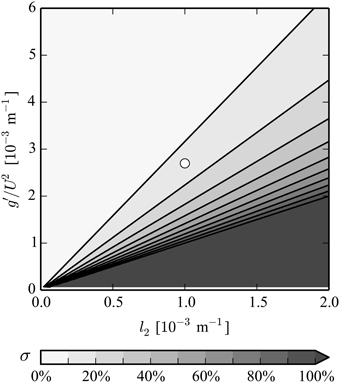
Figure 6. Estimation of the stratification impact on interfacial deep-water waves. Gray shading represents the values of $\sigma ={\left[l_2∕(g\prime ∕U^2)\right]}^2$. The white dot shows the flow configuration of the observed lee wave case.

The considerations expressed above are rigorously valid only if kh₁ ≫ 1. If this condition applies, then σ (and hence the difference between λ_IIW and λ_FIW) is independent of the layer depth h₁. However, this is not the case if the layer depth is relatively shallow (Figure 5B).

For the case in exam here, the layer depth can be shown to have only a marginal impact on the lee wavelength. With the deep-water approximation (that is, neglecting the influence of the lower layer depth), Equation (16) leads to σ = 0.14. Without the deep-water approximation (that is, preserving the influence of the lower layer depth), σ can be estimated on the basis of the relative difference between λ_IIW and λ_FIW from any panel in Figure 5: σ = (λ_IIW − λ_FIW)∕λ_FIW ≈ 0.8∕4.2 = 0.19. This means that the wavenumber of the interfacial wave increases due to stratification in the free atmosphere by 19% (white dot in Figure 6). The close agreement with the estimate from Equation (16) (σ = 14%) indicates that the deep-water approximation is valid in this case.

Given the good agreement between wavelength estimates that are subject to and independent of the short-wavelength approximation, we expect that using σ to assess the importance of stratification effects on interfacial waves beneath the stable layer will give accurate results for most interfacial lee wave observations.

5.2. Impact of Free-atmospheric Stratification on the Shallow-water Approximation

Mountains excite a continuous spectrum of vertically-propagating wave modes if the atmosphere is continuously stratified. In two-layer flow, as shown above, part of these modes become trapped at the interface between the fluid layers. In particular, only relatively short modes satisfying k > l₂ are trapped. In what follows, we use this trapping criterion to investigate the validity of the long-wave approximation, which is a fundamental assumption in shallow-water theory, in the presence of a stably stratified upper layer.

Multiplying the terms in the inequality above by h₁ yields kh₁ > l₂h₁. On the other hand, the long-wave (or shallow-water) approximation, $\text{coth}(k{h}_1)\approx {(k{h}_1)}^{-1}$, is only valid when kh₁ ≪ 1. Scale analysis suggests that the two conditions kh₁ > l₂h₁ (under which interfacial waves exist) and kh₁ ≪ 1 (under which they can be treated with the shallow-water approximation) can be incompatible.

Typical values for the order of magnitude of the Scorer parameter and the layer depth are respectively ${O}(l_2)=10^{-3}$ and ${O}(h_1)=10^3$, hence ${O}$(l₂h₁) = 1. In this case, the shallow-water approximation is clearly inappropriate. The range of values of l₂ and h₁ for which the approximation remains valid can be estimated from the ratio between the transcendental term in Equation (7), coth(kh₁), and its shallow-water approximation form, ${(k{h}_1)}^{-1}$. This ratio is equal to unity if the approximation is accurate. The inaccuracy is hence quantified by the deviation of the ratio from unity, considering the longest possible trapped mode (k = l₂):

$\begin{array}{ll}ϵ=1-(l_2{h}_1)·\text{coth}(l_2{h}_1).& (17)\end{array}$

The dependence of ϵ on l₂ and h₁ is shown in Figure 7. Clearly, stratification aloft (l₂) can cause large deviations from ideal shallow-water behavior, easily exceeding ϵ = 50% for fairly typical atmospheric conditions. For the Desertas case, ϵ ≈ 30%. We conclude that the non-hydrostatic linear frameworks presented in Section 2 are far more accurate than the shallow-water framework in describing the propagation properties of interfacial waves. This is especially the case, when the overlying free atmosphere is stably stratified.

FIGURE 7

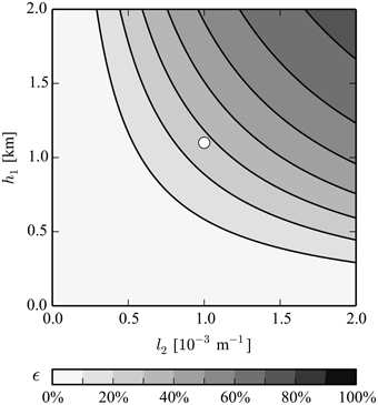
Figure 7. Estimation of the error due to stratification effects in the shallow-water approximation. Gray shading and contours represent the values of ϵ = 1−(l₂h₁) · coth(l₂h₁). The white dot shows the flow configuration of the observed lee wave case.

6. Summary and Conclusions

Lee-wave cloud patterns, frequently observed downstream of islands, are often attributed to the presence of resonant gravity waves. Rigorously, resonant waves are expected to develop if the potential temperature profile is continuous and includes a stable layer below a neutral (or less stable) one. In the case of the marine boundary layer, one instead finds a nearly neutral layer capped by a sharp inversion, which can be thought of as a discontinuity in the potential temperature profile. Lee waves may be more appropriately interpreted as interfacial waves in this case.

Using the results of a linear two-layer flow model to explain the lee wavelength in observations taken in the Madeira archipelago, we highlight the large impact that free-atmospheric stability has on interfacial waves at the boundary-layer capping inversion. Through use of linear theory, we demonstrate that interfacial waves are affected by stable stratification aloft (i.e., by an overlying wave-permitting layer) in two ways:

- First, stratification in the upper layer limits the possible range of lee wavelengths. This happens because wave modes with $k^2<l_2^2$ propagate vertically in the upper layer, without being trapped at the interface (Vosper, 2004). From this criterion, we derived the critical (minimum) values of inversion strength (Δθ_crit, Equation 8) and height (h_1crit, Equation 9) for wave trapping. We showed that waves on an inversion where Δθ = Δθ_crit, or equivalently h₁ = h_1crit, are dynamically identical to surface water waves (see Section 2.2), i.e., they are described by identical FDRs. This equivalence is only possible if the atmosphere above the inversion is stably stratified.

- Second, the wavelength of interfacial disturbances decreases with increasing stratification in the upper layer. In the short-wave limit (kh₁ ≫ 1), the parameter $\sigma ={\left[l_2∕(g\prime ∕U^2)\right]}^2$ quantifies the relative difference between the length of interfacial waves in flow with a neutral and a stratified upper layer. If σ is small, stratification in the free atmosphere has a negligible impact on interfacial waves riding along the inversion.

Furthermore, we show that the shallow-water (or long-wave) approximation (kh₁ ≪ 1) may give an inaccurate description of interfacial waves in atmospheric flows when the upper layer is stably stratified. This is because inversions only trap short wave modes ($k^2>l_2^2$). In fact, the two criteria $k^2>l_2^2$ and kh₁ ≪ 1 are generally incompatible for typical values of h₁ and l₂ in the atmosphere. Conversely, interfacial waves in such conditions are more properly described with the non-hydrostatic linear frameworks presented in Section 2. The deep-water approximation is more appropriate in this case.

A major limitation of this study is that it is restricted to flows with constant background wind speed U. Vertical variability in the horizontal wind profile is known to affect wave propagation by creating wave ducts in regions with high curvature, (1∕U)(d²U∕dz²), which typically coincide with jets. Furthermore, sharp wind speed gradients, typically occurring across temperature inversions, favor the onset of shear instability (e.g., Kelvin-Helmholtz billows). We note here that the FDR of Kelvin-Helmholtz waves in a two-layer discontinuous density profile (see, e.g., Nappo, 2012) converges to that of internal interface waves (Equation 2), for vanishing wind speed difference across the interface. An accurate investigation of the impact of wind speed variability on interfacial waves is, however, outside the scope of this work, and is left for future investigation.

Conflict of Interest Statement

The authors declare that the research was conducted in the absence of any commercial or financial relationships that could be construed as a potential conflict of interest.

Acknowledgments

We thank the reviewers of this paper for their comments and suggestions. This study was supported by the FWF (Austrian Science Fund) grant P24726-N27 to the University of Vienna. NCAR is sponsored by the National Science Foundation.

Footnotes

1. ^Interfacial wave theory is in turn related to hydraulic theory. Hydraulic theory is based on the analogy between the flow of a compressible gas and the flow of a shallow liquid, and is inherently hydrostatic. In contrast, no a priori assumption about hydrostaticity is made in interfacial wave theory.

References

Airy, G. B. (1841). “Tides and waves,” in Encyclopaedia Metropolitana (1817–1845), Mixed Sciences, Vol. 3, eds H. J. Rose, H. J. Rose, and E. Smedley (London: B Fellowes), 241–396.

Baines, P. G. (1995). Topographic Effects in Stratified Fluids. Cambridge: Cambridge University Press.

Craik, A. D. (2004). The origins of water wave theory. Annu. Rev. Fluid Mech. 36, 1–28. doi: 10.1146/annurev.fluid.36.050802.122118

CrossRef Full Text | Google Scholar

Doyle, J. D., Volkert, H., Dörnbrack, A., Hoinka, K. P., and Hogan, T. F. (2002). Aircraft measurements and numerical simulations of mountain waves over the central Alps: a pre-MAP test case. Q. J. R. Meteorol. Soc. 128, 2175–2184. doi: 10.1256/003590002320603601

CrossRef Full Text | Google Scholar

Durran, D. R. (1986a). Another look at downslope windstorms. Part I: the development of analogs to supercritical flow in an infinitely deep, continuously stratified fluid. J. Atmos. Sci. 43, 2527–2543. doi: 10.1175/1520-0469(1986)043<2527:ALADWP>2.0.CO;2

CrossRef Full Text | Google Scholar

Durran, D. R. (1986b). “Mountain waves,” in Mesoscale Meteorology and Forecasting, ed P. S. Ray (Boston, MA: American Meteorological Society), 472–492.

Georgelin, M., and Lott, F. (2001). On the transfer of momentum by trapped lee waves: case of the IOP 3 of PYREX. J. Atmos. Sci. 58, 3563–3580. doi: 10.1175/1520-0469(2001)058<3563:OTTOMB>2.0.CO;2

CrossRef Full Text | Google Scholar

Gill, A. E. (1982). Atmosphere-Ocean Dynamics. London: Academic Press.

Google Scholar

Grubišić, V., Sachsperger, J., and Caldeira, R. M. (2015). Atmospheric wake of Madeira: first aerial observations and numerical simulations. J. Atmos. Sci. doi: 10.1175/JAS-D-14-0251.1. [Epub ahead of print].

CrossRef Full Text | Google Scholar

Houze, R. A. (2014). Cloud Dynamics. Oxford: Academic Press.

Google Scholar

Jarvis, A., Reuter, H. I., Nelson, A., and Guevara, E. (2008). Hole-filled SRTM for the Globe Version 4. Available from the CGIAR-CSI SRTM 90m Database. Available online at: http://srtm.csi.cgiar.org

Jiang, Q. (2014). Applicability of reduced-gravity shallow-water theory to atmospheric flow over topography. J. Atmos. Sci. 71, 1460–1479. doi: 10.1175/JAS-D-13-0101.1

CrossRef Full Text | Google Scholar

Jiang, Q., and Smith, R. B. (2001). Ideal shocks in 2-layer flow. Part II: under a passive layer. Tellus A 53, 146–167. doi: 10.1034/j.1600-0870.2001.00097.x

CrossRef Full Text | Google Scholar

Klemp, J., and Lilly, D. (1975). The dynamics of wave-induced downslope winds. J. Atmos. Sci. 32, 320–339. doi: 10.1175/1520-0469(1975)032<0320:TDOWID>2.0.CO;2

CrossRef Full Text | Google Scholar

Nappo, C. J. (2012). An Introduction to Atmospheric Gravity Waves, 2 Edn. London: Academic Press.

Google Scholar

Ralph, F. M., Neiman, P. J., Keller, T. L., Levinson, D., and Fedor, L. (1997). Observations, simulations, and analysis of nonstationary trapped lee waves. J. Atmos. Sci. 54, 1308–1333. doi: 10.1175/1520-0469(1997)054<1308:Osaaon>2.0.Co;2

CrossRef Full Text | Google Scholar

Scorer, R. S. (1949). Theory of waves in the lee of mountains. Q. J. R. Meteorol. Soc. 75, 41–56. doi: 10.1002/qj.49707532308

CrossRef Full Text | Google Scholar

Scorer, R. S. (1997). Dynamics of Meteorology and Climate. Chichester: Wiley.

Google Scholar

Smith, R. B. (1979). The influence of mountains on the atmosphere. Adv. Geophys. 21, 87–230.

Google Scholar

Teixeira, M. A. (2014). The physics of orographic gravity wave drag. Front. Phys. 2:43. doi: 10.3389/fphy.2014.00043

CrossRef Full Text | Google Scholar

Teixeira, M. A., Argaín, J. L., and Miranda, P. M. (2013). Orographic drag associated with lee waves trapped at an inversion. J. Atmos. Sci. 70, 2930–2947. doi: 10.1175/JAS-D-12-0350.1

CrossRef Full Text | Google Scholar

Turner, J. S. (1973). Buoyancy Effects in Fluids. Cambridge: Cambridge University Press.

Google Scholar

Vosper, S. B. (2004). Inversion effects on mountain lee waves. Q. J. R. Meteorol. Soc. 130, 1723–1748. doi: 10.1256/qj.03.63

CrossRef Full Text | Google Scholar

Vosper, S. B., Wells, H., Sinclair, A., and Sheridan, P. F. (2012). A climatology of lee waves over the UK derived from model forecasts. Meteorol. Appl. 20, 466–481. doi: 10.1002/met.1311

CrossRef Full Text | Google Scholar

Wurtele, M., Sharman, R., and Datta, A. (1996). Atmospheric lee waves. Annu. Rev. Fluid Mech. 28, 429–476.

Google Scholar

Appendix

Frequency Dispersion Relationship for Trapped Lee Waves

The Taylor-Goldstein equation can be derived from the two-dimensional Euler equations (subject to the Boussinesq approximation), the first law of thermodynamics and the incompressible mass continuity equation after linearization and by postulating the existence of wavelike solutions (see, e.g., Nappo, 2012):

$\begin{array}{ll}\frac{d^2ŵ}{d{z}^2}+\left[l^2-k^2\right]ŵ=0.& (\text{A}1)\end{array}$

We solve this equation in two fluid layers by assuming that wave solutions are stationary in both the lower (subscript 1) and the upper one (subscript 2):

$\begin{array}{lll}\hfill {ŵ}_1=A_1{e}^{i{m}_{1}z\prime }+B_1{e}^{-i{m}_{1}z\prime }& & (\text{A}2)\end{array}$

$\begin{array}{lll}\hfill {ŵ}_2=A_2{e}^{i{m}_{2}z\prime }+B_2{e}^{-i{m}_{2}z\prime }.& & (\text{A}3)\end{array}$

Here $ŵ={\left[{\rho }_s∕{\rho }_0(z)\right]}^{-1∕2}·\tilde{w}$, where $\tilde{w}$ denotes a Fourier component of the vertical wind speed perturbation, and ρ_s and ρ₀ the surface density and the unperturbed density profile respectively; $z\prime =z-h_1$, where h₁ is the thickness of the lower layer.

Four boundary conditions (BCs) are required to close the system. The first two are the parallel flow condition at the surface and a radiation condition in the upper layer. For simplicity, we assume flat terrain with constant interface height (z′ = 0), a realistic scenario for a lee wave that propagates above a flat surface after being excited by a mountain. The corresponding BCs become then

$\begin{array}{lll}\hfill {ŵ}_1(z\prime =-h_1)=0& & (\text{A}4)\end{array}$

$\begin{array}{lll}\hfill B_2=0.& & (\text{A}5)\end{array}$

The other two conditions are the kinematic and the dynamic BC at the interface (z′ = 0), which consists of a potential temperature jump with reduced gravity $g\prime =g·\Delta \theta ∕{\theta }_0$. The former condition ensures continuous vertical wind speed, while the latter requires continuous pressure across the θ discontinuity. Following Klemp and Lilly (1975) and Vosper (2004), the kinematic and dynamic BCs are respectively:

$\begin{array}{lll}\hfill {ŵ}_1={ŵ}_2& & (\text{A}6)\end{array}$

$\begin{array}{lll}\hfill \frac{d{ŵ}_1}{dz}-{ŵ}_1\frac{g\prime }{U^2}=\frac{d{ŵ}_2}{dz}.& & (\text{A}7)\end{array}$

Imposing the constraints (A4)–(A7) on Equations (A2) and (A3) and solving for A₁ and B₁ leads to:

$\begin{array}{lll}\hfill A_1=\frac{A_2}{1-e^{-2i{m}_1{h}_1}}& & (\text{A}8)\end{array}$

$\begin{array}{lll}\hfill B_1=\frac{A_2}{1-e^{2i{m}_1{h}_1}}.& & (\text{A}9)\end{array}$

Both coefficients depend on the amplitude A₂ of the interfacial disturbance. Substituting Equations (A5)–(A9) in Equations (A2) and (A3) and eliminating A₂ results finally in a condition that relates the wind speed with the vertical wave numbers m_{1, 2}

$\begin{array}{ll}{U}^2=\frac{g\prime }{i{m}_1\text{coth}\left(i{m}_1{h}_1\right)-i{m}_2}.& (\text{A}10)\end{array}$

Equation (A10) is the frequency dispersion relationship that describes interfacial waves on an inversion between two continuously stratified fluid layers.

Two-dimensional Trapped Lee Wave Model

The two-dimensional wave fields in Figure 4 are obtained by determining the coefficients A₁, A₂, B₁ and B₂ in Equations (A2) and (A3) after imposing a parallel flow condition along topography. Equation (A4) is therefore replaced by:

$\begin{array}{cc}{\widehat{w}}_1(z\prime =-h_1)=U\frac{dH}{dx}=i\widehat{h}kU{e}^{ikx},& \left(\text{A}11\right)\end{array}$

where H is the height and $\widehat{h}$ is the Fourier-series expansion of the terrain profile. Using again (A5)–(A7), and (A11) in Equations (A2) and (A3) yields:

$\begin{array}{lll}\hfill A_1={ŵ}_{1(z\prime =-h_1)}{e}^{i{m}_1{h}_1}-B_1{e}^{2i{m}_1{h}_1}& & (\text{A}12)\end{array}$

$\begin{array}{lll}\hfill B_1={ŵ}_{1(z\prime =-h_1)}\frac{\alpha ·e^{i{m}_1{h}_1}}{\beta +\alpha ·e^{2i{m}_1{h}_1}}& & (\text{A}13)\end{array}$

where $\alpha =i\left(m_1-m_2\right)-\frac{g\prime }{U^2}$ and $\beta =i\left(m_1+m_2\right)+\frac{g\prime }{U^2}$. In the upper layer,

$\begin{array}{lll}\hfill A_2={ŵ}_{1(z\prime =-h_1)}·e^{i{m}_1{h}_1}+B_1·(1-e^{2i{m}_1{h}_1})& & (\text{A}14)\end{array}$

$\begin{array}{lll}\hfill B_2=0.& & (\text{A}15)\end{array}$

The full solution in a domain of n horizontal grid points and a length D = nΔx is computed independently at each level by summing up all Fourier components:

$\begin{array}{cc}{w\prime }_{1,2}(x,z)={[{\rho }_s/{\rho }_0(z)]}^{1/2}·\text{Re}\left[\frac{1}{n}{\displaystyle \sum _{k=0}^{k=2\pi /D}{\widehat{w}}_{1,2}(x,z)}\right].& \left(\text{A}16\right)\end{array}$

Horizontal wind speed perturbations $u_{1,2}^{\prime }$ are determined in a similar fashion, using the incompressibility constraint û_{1, 2} = −(m_{1, 2} ∕ k) · ŵ_{1, 2}.

Since the model described above is solved numerically in spectral space, the boundary conditions are necessarily periodic. This is a critical aspect for trapped lee wave solutions, which are asymmetric with respect to the mountain and do not decay with distance downstream of it. We solve this problem by including an artificial ghost-mountain in the domain, downstream of the first. The distance between the two mountains is set so as to achieve complete destructive interference of the lee wave train. The flow field becomes then symmetric. Figure 4 only shows the left half of the domain.