MSP-Tool: A VBA-Based Software Tool for the Analysis of Multispecimen Paleointensity Data

Introduction

The magnetic field of the Earth is generated in its liquid outer core by magnetohydrodynamic processes. In order to better understand these processes, we need more information on how the field behaved in the past, both in terms of its direction and its intensity. However, while it is fairly straightforward to determine paleodirections from lavas or in-situ archeological artifacts, it is much more difficult to obtain reliable paleointensities from them (e.g., Tauxe and Yamazaki, 2007).

For low, Earth-like fields, a thermoremanent magnetization (TRM), as found in lavas or pottery, is proportional to its inducing field (e.g., Muxworthy and McClelland, 2000). So, by comparing the ancient natural remanent magnetization (NRM) to a TRM imparted in a known laboratory field, the absolute ancient field intensity can be recovered. However, many lavas alter thermochemically during the acquisition of a full TRM. Several methods to mitigate or at least detect this alteration have been proposed. In the classic Thellier-Thellier method (Thellier and Thellier, 1959; later modifications by e.g., Coe, 1967; Aitken et al., 1988; Riisager and Riisager, 2001; Yu et al., 2004) pTRMs are imparted by heating samples stepwise to increasingly elevated temperatures. Lower-temperature steps can be repeated to test for the onset of alteration (pTRM checks; Coe, 1967). The microwave method (e.g., Hill and Shaw, 1999; Suttie et al., 2010) uses the same protocols, but the amount of heating the samples experience is reduced by directly exciting the magnetic spin system using microwaves instead of heating the sample in an oven.

An alternative approach is the multispecimen protocol (Dekkers and Böhnel, 2006; Fabian and Leonhardt, 2010). In contrast to Thellier-style experiments, the multispecimen protocol uses one temperature and multiple fields. In the original multispecimen protocol (MSP-DB; Dekkers and Böhnel, 2006), sister samples are heated only once in-field. Biasing effects induced by pTRM tails are minimized by aligning the specimens' NRMs parallel to the field in the oven. The temperature of the MSP experiment is selected based on the specimen's alteration temperature, the temperature at which a sample starts to show irreversible behavior in its susceptibility-vs.-temperature plot. Evidently, the MSP experiment should be performed below that temperature. Additionally, the ARM test (de Groot et al., 2012) can be used to assess (chemical or magnetic) alteration at the intended MSP temperature.

Fabian and Leonhardt (2010) showed that the original claim of domain-state independence is not entirely correct and suggested three additional steps to estimate the amount of NRM lost, to detect (and correct for) multidomain behavior and to detect chemical alteration. These three steps can also be used to calculate several parameters that give valuable information about the samples' domain state and to calculate single-specimen paleointensity estimates and intrinsic error estimates. This protocol is referred to as MSP-DSC, where DSC stands for “domain-state-corrected.” The two multispecimen protocols have been used by e.g., Michalk et al. (2008, 2010), Böhnel et al. (2009), Muxworthy and Taylor (2011), de Groot et al. (2013a,b), Monster et al. (2015), and Tema et al. (2015).

A popular software tool for the analysis of Thellier-style paleointensity experiments is ThellierTool 4.0 (Leonhardt et al., 2004). More recently, Shaar and Tauxe (2013) introduced Thellier GUI. The software tool described here is designed for the analysis of multispecimen paleointensity experiments. The program was written in Visual Basic for Microsoft Excel (Office 2010, Windows). It calculates and plots multispecimen data and provides checks on the reliability of the results. In addition, it also estimates the amount of NRM remaining and pTRM gained and uses these to correct for possible misalignment.

The Multispecimen Protocol

In the original multispecimen protocol (Dekkers and Böhnel, 2006), the specimens are only heated once (m₁, with m₀ being the NRM). In the DSC protocol (Fabian and Leonhardt, 2010) three additional steps are added (m₂ to m₄). The five measurements are then:

m₀: NRM

m₁: Magnetization after heating and cooling in parallel field

m₂: Magnetization after heating and cooling in anti-parallel field

m₃: Magnetization after heating in zero-field and cooling in parallel field

m₄: Same as m₁ (progressive alteration check)

From these five measurements of the vector remanence, the paleointensity is determined for a lava flow. The original MSP-DB method assumes that multidomain effects are negligible. In this case, if the laboratory field is equal to the paleofield, m₁ should be equal to m₀ (and lower or higher if the laboratory field is lower or higher, respectively, than the paleofield). The Q_DB ratio (Dekkers and Böhnel, 2006) is defined as follows:

$\begin{array}{rc}{Q}_{DB}=\frac{m_1-m_0}{m_0}& (1)\end{array}$

where m₀ and m₁ are the scalar intensities of the two remanences. The fraction-corrected (MSP-FC) and domain-state corrected (MSP-DSC) ratios (both defined in (Fabian and Leonhardt, 2010)) are:

$\begin{array}{rc}{Q}_{FC}=2·\frac{m_1-m_0}{2m_0-m_1-m_2}& (2)\end{array}$

$\begin{array}{rc}{Q}_{DSC}=2·\frac{{\left(1+\alpha \right)m}_1-m_0-\alpha m_3}{2m_0-m_1-m_2}& (3)\end{array}$

The denominator in both equations is equal to twice the amount of NRM lost. The ratios are therefore normalized to the demagnetized part of the NRM rather than to the complete NRM as is the case for the DB ratio. As the fraction NRM lost is often not the same even for samples within one cooling unit, this fraction correction should reduce the amount of scatter (Fabian and Leonhardt, 2010). At H_lab = 0μT, m₁-m₀ is equal to minus the amount of NRM lost and therefore the y intercept should be at (0, −1). Alteration, domain-state effects or alignment errors, however, may lead to a different intercept. The intercept can thus serve as a reliability check.

The parameter α in the numerator of Q_DSC is used to correct the FC ratio for domains state effects. Fabian and Leonhardt (2010) empirically tested different values for α using synthetic samples with different unblocking temperatures and domain states. α was shown to range typically between 0.2 and 0.8, where α ≈ 0.5 yielded best results, although Fabian and Leonhardt (2010) do note that the value of α is likely site-specific. α = 0.5 was used in e.g., de Groot et al. (2013a, 2015) and Monster et al. (2015). Tema et al. (2015) observed very little difference when changing the value of α for their kiln samples and chose α = 0.5. Muxworthy and Taylor (2011), however, found that for their samples α = 0 yielded the best results. In this case the DSC ratio reduces to the FC ratio.

Apart from these three ratios, a number of parameters estimating the domain state, progressive alteration, and the total (domain-state-induced and alteration-induced) error can be calculated. Further explanation of these parameters is provided in Fabian and Leonhardt (2010), in the electronic supplement, and in the “list of parameters” sheet in MSP-Tool.

The VBA Tool

The MSP-tool workbook consists of several sheets: “manual”; “input”; “parameters”; “parameters, corrected”; and “list of parameters.” Additionally, several plots (MSP-DB, MSP-FC, and MSP-DSC) are provided that can be exported as PNG or CSV files. File actions and calculations are easily carried out by clicking the corresponding button. The user interface is shown in Figure 1. MSP-Tool, as well as several input files, can be found in the Supplementary Material or downloaded from MSP-Tool.org.

FIGURE 1

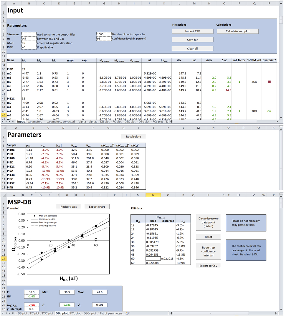
Figure 1. User interface, from top to bottom: the “input” sheet, the “parameters” sheet and one of the “plot” sheets (MSP-DB).

The “Input” Sheet: Data Format and Directional Checks

The “input” sheet is the start sheet. It provides buttons to import, save, and clear data and to carry out the actual MSP calculations. Furthermore, the values of several parameters, such as the α parameter (Fabian and Leonhardt, 2010) and the maximum acceptable angular deviation (AAD) between the pTRMs and the NRMs, can be set here. α's default value is 0.5 and the AAD is set to 10 degrees. If applicable, the expected paleointensity value may be entered to enable calculating the intensity error fraction (IEF; Biggin et al., 2007).

MSP-Tool supports two different input formats. Data can be imported using either the three Cartesian components of the remanence or using the intensity, declination and inclination of the remanence (which are automatically converted to Cartesian components). The order of magnitude for every line of data must be the same; if not, for example for data measured on a JR-6 spinner magnetometer, an additional (sixth) column with the exponent can be added. Since the MSP calculations are inherently relative, the units for m_x, m_y, m_z and the intensity can be chosen freely, as long as they are the same for all five measurement steps.

Clicking the “Calculate and plot” button calculates all parameters in the “input” and “parameters” sheets and plots the three ratios in the “plot” sheets. The VBA tool can process all three MSP protocols and will calculate and plot the relevant ratios and parameters accordingly.

The isolated pTRMs (columns G to I) are calculated by first estimating the vector NRM remaining. The latter is obtained by adding the vectors m₁ and m₂ and dividing the result by 2, c.f. the fraction-corrected MSP-FC ratio (Fabian and Leonhardt, 2010):

$\begin{array}{rc}\text{NRM remaining}=\frac{{\text{m}}_1+{\text{m}}_2}{2}& (4)\end{array}$

The vector pTRMs are then:

$\begin{array}{rc}{\text{pTRM}}_i={\text{m}}_i-\text{NRM}\text{remaining}& (5)\end{array}$

The scalar magnetic moments m₀ to m₄ (column J) are simply the magnitudes of the vector remanences m₀ to m₄, whereas the alignment-corrected intensities (column K) are obtained by adding up the isolated NRM remaining and the pTRMs. Of course, if the pTRM is parallel to the NRM, m_{i, corr} = m_i.

$\begin{array}{rc}{m}_i=\sqrt{m_{i,x}^2+m_{i,y}^2+m_{i,z}^2}& (6)\end{array}$

$\begin{array}{rc}{m}_{i,corr}=\left|\text{NRM}\text{remaining}\right|+{\left|\text{pTRM}\right|}_i& (7)\end{array}$

Columns L and M show the declination (between 0 and 360°) and inclination (between −90 and +90°) of the m₀ to m₄ steps. All declinations and inclinations are given in specimen coordinates. The declinations and inclinations of the isolated NRM remaining and the isolated pTRMs are used to calculate the parameters Δdec and Δinc (columns N and O), which are a measure of how well the specimens were aligned to the laboratory field. If Δdec and Δinc exceed the AAD, they are shown in red. We chose to use Δdec and Δinc rather than a single angular difference because using these two parameters it is easier to spot systematic alignment errors. Please note that in case of large overprints Δdec and Δinc may be high even if the pTRM was aligned perfectly with the NRM (m₀).

$\begin{array}{rc}△\text{dec}=|{\text{dec}}_{\text{pTRM}}-{\text{dec}}_{\text{NRM remaining}}|& (8)\end{array}$

$\begin{array}{rc}△\text{inc}=|{\text{inc}}_{\text{pTRM}}-{\text{inc}}_{\text{NRM remaining}}|& (9)\end{array}$

These calculations all implicitly assume that even if the specimens were not aligned properly, at least they were aligned consistently, i.e., that the pTRMs of heating steps 1 and 2 are exactly anti-parallel to each other, even if they are not exactly parallel (m₁) or anti-parallel (m₂) to the NRM. This is a valid assumption if the positions of the sample holders with respect to the furnace were not changed during the experiment. To minimize orientation issues, it is advisable to process each individual specimen on the same holder throughout the experiment, eliminating the need to orient holders for each step in the MSP-DSC experiment. As the alignment correction does not take into account multidomain effects such as pTRM tails, a proper alignment of the samples during the experiment is still paramount—it is merely a tool to suppress unavoidable small experimental misalignments.

The “m2 factor” (column P) is the normalized dot product of m₀ and m₂. This parameter equals +1 when m₀ and m₂ are parallel and -1 when they are antiparallel. m₂ is multiplied by this factor to correct for “negative” m₂ intensities. Not correcting for this often results in plots with a large amount of scatter (see Figure S3). The “m2 factor” is similar to using vector subtraction (see e.g., Muxworthy and Taylor, 2011) instead of scalar subtraction.

Finally, the angle between the NRM lost and the NRM remaining is calculated (Equation 10). If this angle exceeds the AAD, a warning is shown in column R. A large difference may indicate the presence of an overprint, which would invalidate the result. Alternatively, if the sample's alignment was changed between the first two steps, the NRM remaining cannot be accurately calculated and the angular difference between the NRM remaining and the NRM gained may be anomalously high.

$\begin{array}{rc}\theta ={cos}^{-1}\frac{{\text{NRM}}_{lost}·{\text{NRM}}_{remaining}}{\parallel {\text{NRM}}_{lost}\parallel \parallel {\text{NRM}}_{remaining}\parallel }& (10)\end{array}$

The “Parameters” Sheet

The “parameters” and “parameters, corrected” sheets show a number of parameters that were proposed by Fabian and Leonhardt (2010). These include a measure of the domain state μ_DS, the progressive alteration ε_alt, single-specimen estimates of the paleointensity H_max and H_est and estimates of the alteration error and domain-state error. In the “parameters” sheet these are calculated from the uncorrected remanences m₀ to m₄, whereas the “parameters, corrected” sheet uses the alignment-corrected remanences.

The progressive alteration is defined in a slightly different way than in Fabian and Leonhardt (2010). Instead of the absolute value of m₁-m₄ normalized by m₁, we use:

$\begin{array}{rc}{\epsilon }_{alt}=\frac{m_4-m_1}{m_1}& (11)\end{array}$

This helps to distinguish between measurement noise (which averages to zero) and a systematic (alteration-induced) error. Fabian and Leonhardt's (2010) alteration error is shown in column D as |ε_alt|. For definitions of the parameters H_est, H_max and three error estimates ΔQ_{DSC, alt}, ΔQ_{DSC, ds} and Δ Q_i see Fabian and Leonhardt (2010).

The “Plot” Sheets: Data Presentation, Statistics, and Reliability Checks

The plot sheets (DB, FC, DSC, and their alignment-corrected versions) show a plot and a table of the data points as well as the calculated paleointensity and its error bounds and two reliability checks: the average alteration parameter ${\overline{\epsilon }}_{alt}$ and the difference between the theoretical and experimental intersection with the y axis Δb. The latter is only applicable to the fraction-corrected plots (i.e., MSP-FC and MSP-DSC). If the linear regression does not pass through (0, −1), this may indicate a problem in the experiment; the linear regression is therefore not forced through this point. Outliers can be removed by selecting the relevant cell in the “used” or “discarded” column and clicking “Discard/restore data point” or using the keyboard shortcut CTRL+d. The plot sheets also show the values of r² and χ² of the linear regression, where χ² is defined as the mean quadratic deviation between the measured value of the DB, FC or DSC ratio (Q_{i, measured}) and the value of the linear regression at that laboratory field (Q_{i, expected}):

$\begin{array}{l}{\chi }^2=\frac{\sum {\left(Q_{i,measured}-Q_{i,expected}\right)}^2}{N}\end{array}$

Clicking “Bootstrap confidence interval” calculates and plots the bootstrap average and the confidence interval. The confidence level may be changed in the “input” sheet; its default value is 95%. The bootstrap function resamples the data set with replacement within their error bounds and calculates a linear fit for each bootstrap cycle. Bootstrap cycles that have a standard deviation of less than 10 μT in their average x coordinate are discarded to prevent fits through data points at one laboratory field (i.e., vertical fits). The confidence interval is constructed by calculating the values of each linear fit at 11 values of the x axis (i.e., field values) between 0 mT and a maximum field value which is the maximum used laboratory field + the minimum used field. For each of the 11 values of x, the values of the linear fits (i.e., the y values) are sorted and the uppermost and lowermost portions of these values (2.5% in case of a 95% confidence level) are cut off. Eleven may seem a rather arbitrary choice, but it empirically proved to yield smooth uncertainty envelopes, whereas a lower number often resulted in significantly more irregularly shaped envelopes. The upper and lower uncertainty boundary of the paleointensity are estimated by linear interpolation between two data points closest to zero on the uncertainty envelope.

The y axes of the plots are scaled automatically by Microsoft Excel, which may result in unrepresentative plots in case of outliers. After discarding the outliers, the y axis can be resized using the “Resize y axis” button. “Export chart” will export the graph as a PNG file. The data points and error envelope may also be exported as CSV files for further processing with an application of choice.

Application

To test MSP-Tool's ability to accurately determine and correct for alignment problems on real rocks, a complete MSP experiment including preliminary ARM test (de Groot et al., 2012; single-core protocol) was applied to two lava flows from Mt Etna (site PI and site TD) that had been given a full TRM in the laboratory by cooling from 600°C in a field of 40 μT. Half of the specimens were deliberately misaligned. Both input files are included in the Supplementary Material.

Preliminary Experiments

Before carrying out the actual MSP experiment, next to the ARM test at the MSP temperature (using 17 field steps of up to 150 mT), some other experiments were conducted to assess the specimens' alteration temperature and domain state. These experiments are described in more detail in the Supplementary Material. The susceptibility-vs.-temperature diagrams for site TD did not show any significant alteration after acquisition of the laboratory full-TRM, whereas site PI showed irreversible behavior at temperatures > 300°C (Figure S1a). Both sites plotted within the pseudo-single domain range on a Day plot (Day et al., 1977), with the full-TRM samples plotting closer to the single-domain field than the original samples, the samples in their NRM state as collected in the field (Figure S1b). Based on the susceptibility- vs.-temperature diagrams, no significant alteration at the selected MSP temperature of 300°C was expected, and the ARM test (de Groot et al., 2012) indeed did not reveal any (Figure S1c). For site PI, however, multiple heatings did induce alteration, as evidenced by its high alteration error ${\overline{\epsilon }}_{alt}$ during the MSP experiment.

The MSP Experiment

After the positive ARM test, the MSP-DSC protocol (Fabian and Leonhardt, 2010) was carried out using five laboratory fields (12, 24, 36, 48, and 60 μT) and two specimens per field level per site. Of the 20 specimens in total, half were aligned correctly, whereas the other 10 were misaligned to the field in the oven under various angles (Δdec = 0, 15, 30, or 90° and Δinc = 0, 15, 30, or 90°). Samples were aligned using a custom-made sample holder (similar to Böhnel et al. (2009), also see Figure S2). The specimens' NRM (m₀) and the four remanences after in-field heating and/or cooling (m₁ to m₄) were measured on an AGICO JR-6 spinner magnetometer.

Results and Observations

In 90% of cases, Δdec and Δinc as calculated by MSP-Tool were within 15° of the intended misalignment angles (see Table S1). For site PI this percentage was higher: 100% of the intended Δdec and Δinc values were reproduced to within 15° of the intended value of the alignment error, of which 95% within 10° and 70% within 5°. For site TD Δdec and Δinc were less precise: 80% was within 15° of the intended alignment error, 65% within 10° and 30% within 5°. It would seem that the Δdec and Δinc parameters are more accurate for larger fractions of NRM lost (c. 30% for PI and 5–10% for TD). Intuitively, this makes sense. If the pTRM is only a small fraction of the total remanence, slight measurement errors may have a larger effect, especially when one of the axes is close to zero (steep tangent) and/or the remanences are measured with few significant digits. It is also interesting to note that the third heating step (zero-field heating, in-field cooling) often yields a distinctly larger Δdec or Δinc than the other steps, which may be related to tail effects.

Looking at the plots (Figure 2), it is apparent that the “alignment-corrected” plots show significantly less scatter than the uncorrected plots, although the correction does not always completely “restore” these data points, highlighting the importance of careful alignment in the MSP experiment. Unsurprisingly, the worst outliers in the standard plots are the specimens with the highest alignment errors: PI10B (Δdec = 90°, Δinc = 0°) at 24 μT, PI13C (Δdec = 90°, Δinc = 30°) at 60 μT, TD4C (Δdec = 0°, Δinc = 90°) at 36μT, and TD6C (Δdec = 90°, Δinc = 90°) at 60 μT.

FIGURE 2

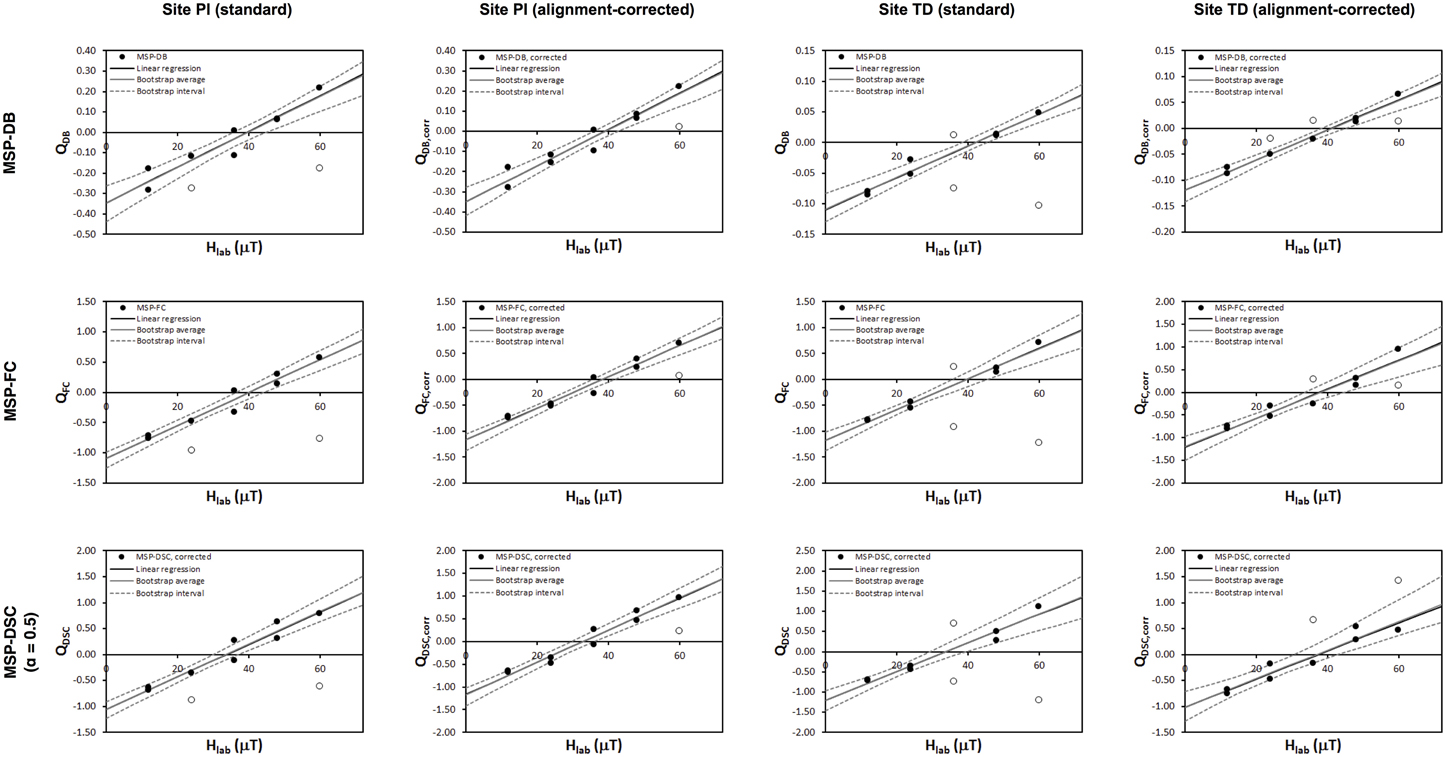
Figure 2. MSP-DB, MSP-FC, and MSP-DSC plots (standard and alignment-corrected) for sites PI and TD which were given a full TRM at 40 μT in the laboratory.

All plots except the DSC plots for site PI and the uncorrected DSC plot for TD reproduced the “paleofield” within error. Lowering the α factor from 0.5 to 0.2 or even 0.0 (in which case MSP-DSC reduces to MSP-FC) improved the “paleointensity” estimate for the DSC protocol (Figure 3). The erroneous result obtained for site PI highlights the importance of the alteration check, as site PI shows nearly 8% progressive alteration, whereas site TD only altered by c. 2%. Since the ARM test (using samples that had been heated only once) was positive, this alteration must have occurred after the first heating step. And indeed the MSP-DB protocol (one heating step) does produce the correct “paleointensity” for site PI.

FIGURE 3

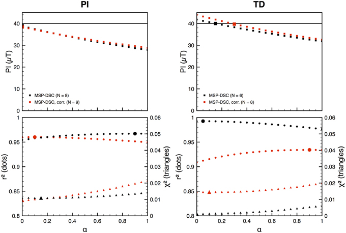
Figure 3. Simulated paleointensity, r², and χ² as a function of the α parameter. The optimal values are indicated by larger symbols. r² and χ² do not change significantly with varying α. The number of samples used in the calculation of the paleointensity N is shown in the legend of the upper figures. For site TD, N increased from 6 to 8 when correcting the data for misalignment; for site PI N increased from 8 to 9.

Discussion

Reliability Criteria

MSP-Tool offers four reliability criteria: two directional criteria (the overprint check, and Δdec and Δinc), the amount of progressive alteration ε_alt, and the intersection with the y axis (not applicable to MSP-DB). A large overprint may be reason to discard individual samples, although an overprint warning may also occur when the alignment of the specimen was altered between steps m₁ and m₂, leading to an inaccurate estimate of the NRM remaining and NRM lost. In case of consistent alignment (i.e. m₁ and m₂ aligned exactly antiparallel) and high Δdec and Δinc, the corrected plots may be preferred. Finally, both the average progressive alteration ${\overline{\epsilon }}_{alt}$ and the Δb intersection criterion are shown on the plot sheets. ${\overline{\epsilon }}_{alt}$ > 3% is considered too high (de Groot et al., 2013a). Theoretically, the linear fits through Q_FC and Q_DSC should pass through (0, −1) as these ratios are normalized to the amount NRM lost rather than the full NRM. Failure to pass through this point (within 10% and/or within error) may indicate that something other than domain-state-related processes is at work and may be a reason to distrust the obtained paleointensity. It is strongly recommended to conduct the ARM test (de Groot et al., 2012) prior to the MSP experiment to test for subtle alteration at the intended MSP temperature.

Alignment Correction

In the alignment correction procedure, the scalar intensities m₁ to m₄ are calculated by adding up the isolated NRM remaining and pTRM gained. The full-TRM experiment showed that this correction functions rather well, although it should be noted that multidomain effects such as tails may influence the calculation of the NRM remaining and therefore the calculated pTRMs. It is also important to note that the alignment correction is only accurate if the samples were aligned exactly antiparallel during the first and second heating steps. In order for the correction to work, therefore, it is important not to change the orientation of the specimens in the oven between MSP steps. As the alignment correction does not 100% restore specimens that were misaligned by a large angle, it is still paramount to align the specimens with care.

Domain-State Correction: The α Factor

Fabian and Leonhardt (2010) recommend a value of 0.5 ± 0.3 as default guess for the α parameter and argue that if a sufficient number of data points is available, α can be optimized such that the mean quadratic deviation between the data points and the linear fit is minimized. By changing the value of the α parameter in the input sheet and re-running the calculation, an optimal value can be determined in MSP-Tool. Like Muxworthy and Taylor (2011) for their Icelandic data set, we found that lower values of the α parameter produced results closer to the expected value (Figure 3). r² value was generally at a maximum and χ² at a minimum for low values of α (α < 0.2), although the differences are small. The “paleointensities” obtained from the uncorrected MSP-DSC plots as a function of α varied between 38.9 (α = 0) and 27.9 μT (α = 1) for site PI and between 41.8 (α = 0) and 31.8 μT (α = 1) for site TD. That PI's result is closer to the expected “paleointensity” for lower values of α may be caused by PI's large progressive alteration. By lowering the α parameter, the influence of the more altered m₃ step is also reduced.

Conclusion and Recommendations for Multispecimen Experiments

MSP-Tool is an easy-to-use VBA-based tool for analyzing multispecimen experiments. It calculates all ratios and parameters from Dekkers and Böhnel (2006) and Fabian and Leonhardt (2010). Additionally, it estimates the amount of NRM remaining and pTRM gained and uses these to estimate and correct for alignment errors. Moreover, it provides important criteria to assess the reliability of the MSP experiment. For an optimal experiment, the following aspects should be taken into account:

• The ARM test (de Groot et al., 2012) is a valuable tool to assess the risk of alteration during the MSP experiment beforehand. If a site does not pass the ARM test at any temperature but is shown to yield an overestimate at T₁ and an underestimate at T₂, the MSP experiment may be carried out at these two temperatures, providing upper and lower bounds of the actual paleofield.

• Misalignment leads to incorrect estimates of the paleofield as the measured vector remanences are shorter (parallel field steps) or longer (antiparallel field step) than the vector NRM remaining plus the vector pTRM lost. This leads to an underestimate of m₁ and therefore of Q_DB, Q_FC, and Q_DSC, and thus an overestimate of the paleofield. MSP-Tool corrects for this by adding up the two separate components (the NRM remaining and the pTRM gained).

• Site PI highlights that a large progressive alteration may lead to underestimates in the DSC protocol. As a successful ARM test implies that no significant alteration occurred after one heating step, the alteration must therefore arise from the multiple heating steps in the MSP experiment. It is recommended to rely on the DB plot in such cases, although it should be recognized that the slope correction and domain state correction cannot be applied.

• As the slope of the DB plot depends on the entire NRM rather than the amount of NRM lost, inhomogeneity between specimens may lead to significant scatter. Selecting specimens based on similar amounts of NRM lost may substantially improve the DB plots.

Author Contributions

The project was designed by MM in conjunction with LdG and MD. MM wrote the VBA code and carried out the experiments. All three authors participated in the data analysis and contributed to the writing of the manuscript.

Conflict of Interest Statement

The authors declare that the research was conducted in the absence of any commercial or financial relationships that could be construed as a potential conflict of interest.

Acknowledgments

This research was funded by a grant (project number 822.01.002) from the Earth and Life Science Division (ALW) of the Netherlands Organization for Scientific Research (NWO). MM would like to thank Cor G. Langereis for his advice regarding the bootstrap statistics used in the VBA code.

Supplementary Material

The Supplementary Material for this article can be found online at: https://www.frontiersin.org/article/10.3389/feart.2015.00086

References

Aitken, M. J., Allsop, A. L., Bussell, G. D., and Winter, M. B. (1988). Determination of the intensity of the earths magnetic-field during archaeological times - reliability of the thellier technique. Rev. Geophys. 26, 3–12. doi: 10.1029/RG026i001p00003

CrossRef Full Text | Google Scholar

Biggin, A. J., Perrin, M., and Dekkers, M. J. (2007). A reliable absolute palaeointensity determination obtained from a non-ideal recorder. Earth Planet. Sci. Lett. 257, 545–563. doi: 10.1016/j.epsl.2007.03.017

CrossRef Full Text | Google Scholar

Böhnel, H. N., Dekkers, M. J., Delgado-Argote, L. A., and Gratton, M. N. (2009). Comparison between the microwave and multispecimen parallel difference pTRM paleointensity methods. Geophys. J. Int. 177, 383–394. doi: 10.1111/j.1365-246X.2008.04036.x

CrossRef Full Text | Google Scholar

Coe, R. S. (1967). Paleo-intensities of the Earth's magnetic field determined from tertiary and quaternary rocks. J. Geophys. Res. 72, 3247–3262. doi: 10.1029/JZ072i012p03247

CrossRef Full Text | Google Scholar

Day, R., Fuller, M., and Schmidt, V. A. (1977). Hysteresis properties of titanomagnetites - grain-size and compositional dependence. Phys. Earth Planet. Inter. 13, 260–267. doi: 10.1016/0031-9201(77)90108-X

CrossRef Full Text | Google Scholar

de Groot, L. V., Béguin, A., Kosters, M. E., van Rijsingen, E. M., Struijk, E. L. M., et al. (2015). Earth and planetary science letters. Earth Planet. Sci. Lett. 419(C), 154–167. doi: 10.1016/j.epsl.2015.03.020

CrossRef Full Text

de Groot, L. V., Biggin, A. J., Dekkers, M. J., Langereis, C. G., and Herrero-Bervera, E. (2013a). Rapid regional perturbations to the recent global geomagnetic decay revealed by a new Hawaiian record. Nat. Commun. 4, 2727–2727. doi: 10.1038/ncomms3727

PubMed Abstract | CrossRef Full Text | Google Scholar

de Groot, L. V., Dekkers, M. J., and Mullender, T. A. T. (2012). Exploring the potential of acquisition curves of the anhysteretic remanent magnetization as a tool to detect subtle magnetic alteration induced by heating. Phys. Earth Planet. Inter. 194, 71–84. doi: 10.1016/j.pepi.2012.01.006

CrossRef Full Text | Google Scholar

de Groot, L. V., Mullender, T. A. T., and Dekkers, M. J. (2013b). An evaluation of the influence of the experimental cooling rate along with other thermomagnetic effects to explain anomalously low palaeointensities obtained for historic lavas of Mt Etna (Italy). Geophys. J. Int. 193, 1198–1215. doi: 10.1093/gji/ggt065

CrossRef Full Text | Google Scholar

Dekkers, M. J., and Böhnel, H. N. (2006). Reliable absolute palaeointensities independent of magnetic domain state. Earth Planet. Sci. Lett. 248, 508–517. doi: 10.1016/j.epsl.2006.05.040

CrossRef Full Text | Google Scholar

Fabian, K., and Leonhardt, R. (2010). Multiple-specimen absolute paleointensity determination: an optimal protocol including pTRM normalization, domain-state correction, and alteration test. Earth Planet. Sci. Lett. 297, 84–94. doi: 10.1016/j.epsl.2010.06.006

CrossRef Full Text | Google Scholar

Hill, M. J., and Shaw, J. (1999). Palaeointensity results for historic lavas from Mt Etna using microwave demagnetization/remagnetization in a modified Thellier-type experiment. Geophys. J. Int. 139, 583–590. doi: 10.1046/j.1365-246x.1999.00980.x

CrossRef Full Text | Google Scholar

Leonhardt, R., Heunemann, C., and Krása, D. (2004). Analyzing absolute paleointensity determinations: acceptance criteria and the software ThellierTool4.0. Geochem. Geophys. Geosyst. 5:Q12016. doi: 10.1029/2004GC000807

CrossRef Full Text | Google Scholar

Michalk, D. M., Biggin, A. J., Knudsen, M. F., Böhnel, H. N., Nowaczyk, N. R., et al. (2010). Application of the multispecimen palaeointensity method to Pleistocene lava flows from the Trans-Mexican Volcanic Belt. Phys. Earth Planet. Inter. 179, 139–156. doi: 10.1016/j.pepi.2010.01.005

CrossRef Full Text | Google Scholar

Michalk, D. M., Muxworthy, A. R., Boehnel, H. N., Maclennan, J., and Nowaczyk, N. (2008). Evaluation of the multispecimen parallel differential pTRM method: a test on historical lavas from Iceland and Mexico. Geophys. J. Int. 173, 409–420. doi: 10.1111/j.1365-246X.2008.03740.x

CrossRef Full Text | Google Scholar

Monster, M. W. L., de Groot, L. V., Biggin, A. J., and Dekkers, M. J. (2015). The performance of various palaeointensity techniques as a function of rock magnetic behaviour – A case study for La Palma. Phys. Earth Planet. Inter. 242, 36–49. doi: 10.1016/j.pepi.2015.03.004

CrossRef Full Text | Google Scholar

Muxworthy, A. R., and McClelland, E. (2000). The causes of low-temperature demagnetization of remanence in multidomain magnetite. Geophys. J. Int. 140, 115–131. doi: 10.1046/j.1365-246x.2000.00000.x

CrossRef Full Text | Google Scholar

Muxworthy, A. R., and Taylor, S. N. (2011). Evaluation of the domain-state corrected multiple-specimen absolute palaeointensity protocol: a test of historical lavas from Iceland. Geophys. J. Int. 187, 118–127. doi: 10.1111/j.1365-246X.2011.05163.x

CrossRef Full Text | Google Scholar

Riisager, P., and Riisager, J. (2001). Detecting multidomain magnetic grains in Thellier palaeointensity experiments. Phys. Earth Planet. Inter. 125, 111–117. doi: 10.1016/S0031-9201(01)00236-9

CrossRef Full Text | Google Scholar

Shaar, R., and Tauxe, L. (2013). Thellier GUI: an integrated tool for analyzing paleointensity data from Thellier-type experiments. Geochemistry 14, 677–692. doi: 10.1002/ggge.20062

CrossRef Full Text | Google Scholar

Suttie, N., Shaw, J., and Hill, M. J. (2010). Earth and planetary science letters. Earth Planet. Sci. Lett. 292, 357–362. doi: 10.1016/j.epsl.2010.02.002

CrossRef Full Text

Tauxe, L., and Yamazaki, T. (2007). “Paleointensities,” in Treatise on Geophysics, Vol. 5, Geomagnetism, ed M. Kono (Amsterdam: Elsevier), 509–563.

Tema, E., Camps, P., Ferrara, E., and Poidras, T. (2015). Directional results and absolute archaeointensity determination by the classical Thellier and the multi-specimen DSC protocols for two kilns excavated at Osterietta, Italy. Stud. Geophys. Geod. 59, 554–577. doi: 10.1007/s11200-015-0413-0

CrossRef Full Text | Google Scholar

Thellier, E., and Thellier, O. (1959). Sur l'intensité du champ magnétique terrestre dans le passé historique et géologique. Ann. Geophys. 1, 37–52.

Yu, Y. J., Tauxe, L., and Genevey, A. (2004). Toward an optimal geomagnetic field intensity determination technique. Geochem. Geophys. Geosyst. 5:Q02H07. doi: 10.1029/2003GC000630

CrossRef Full Text | Google Scholar