Annual Climatology of the Diurnal Cycle on the Canadian Prairies

Introduction

Historically many climate and hydrometeorology studies have been largely based on temperature and precipitation for which long-term records are available (Leung et al., 2003; Betts et al., 2005; Betts, 2007; Koster et al., 2009; Berg et al., 2015). By focusing on temperature and precipitation the importance of cloud cover in modulating the diurnal evolution of temperature and humidity is neglected, thus obscuring the fully coupled nature of the land-atmosphere-cloud system. One exception is Dai et al. (1998) who analyzed the global coupling between cloud cover and the diurnal cycle of temperature over land.

This paper continues the analysis of the diurnal climatology of the Canadian Prairies using the excellent climate station data (Betts et al., 2013a,b, 2014a,b, 2015). In addition to standard hourly climate variables of high quality, these data have a remarkable set of hourly observations of opaque or reflective cloud cover in tenths, made by trained observers who have followed the same protocol for 60 years (MANOBS, 2013). Opaque cloud is defined as cloud that obscures the sun, moon or stars. These opaque cloud observations (estimated as a fraction of the sky in tenths) are sufficiently good that we were able to calibrated daily means of opaque cloud at Regina, Saskatchewan against multiyear shortwave and longwave radiation data from the Baseline Surface Radiation Network (BSRN) station at Bratt's Lake 25 km away (Betts et al., 2015). This gives daily shortwave and longwave cloud forcing (SWCF, LWCF), as well as net radiation, R_n, as a function of daily mean opaque cloud cover. These Prairie data have a full hourly set of temperature, relative humidity, windspeed and direction, precipitation, cloud and derived radiation, as well as snow depth. This broadens and deepens our understanding of the diurnal climatology of the fully coupled land-surface-atmosphere-cloud system. Previously, the coupling between cloud forcing and the diurnal cycle of temperature over land (Betts, 2015) has received rather little quantitative analysis.

Most analyses in our earlier papers (Betts et al., 2013a,b, 2014a,b, 2015) reduced the hourly data to daily means and represented the diurnal cycle climate in terms of maximum, T_x, and minimum temperature, T_n, and the diurnal range of temperature, DTR = T_x–T_n. The difference in relative humidity, RH, between T_n and T_x (RH_tn–RH_tx) was used as an approximation of the diurnal range of RH. Betts et al. (2013a) mapped the impact of daily mean opaque cloud, OPAQ_m, on the diurnal cycle and showed the large differences between summer and winter. Betts et al. (2013b) looked at how the shift from summer fallow to continuous cropping on 5 mega-hectares of farmland, has cooled and moistened the diurnal cycle climate in the growing season, which is consistent with increased transpiration. Betts et al. (2014a) showed how there were sharp transitions between the warm season and cold season associated with snow cover, and therefore with the freezing point of water. Mean temperatures fall 10 K with fresh snow typically in November, mostly due to the increase in the surface albedo, as well as a drop in the downwelling longwave radiation. The reverse transition is seen in spring as the snow-pack melts. The high albedo snow cover acts as a fast climate switch, which not only drops the near-surface temperature by 10 K, but also transforms the surface-cloud coupling from an unstable daytime boundary layer (BL), controlled by SWCF without snow cover, to a stable BL dominated by LWCF with snow cover. This climate switch is so strong that the interannual variability of the mean October to April (when snow may occur) has a linear relation to the fraction of days with snow cover (Betts et al., 2014a). In the warm season without snow, Betts et al. (2014b) looked at the coupling between opaque cloud and lagged precipitation anomalies and the anomalies of DTR and RH_tx on monthly, seasonal and 50-yr timescales; and constructed a simplified energy and water budget for the growing season on the Prairies. Betts et al. (2015) recalibrated the opaque cloud data in terms of SWCF and LWCF for T <> 0°C using 17 years of BSRN data; and showed the dependence in summer (but not winter) of the diurnal range of temperature and humidity on windspeed, RH, day-night asymmetries in the opaque cloud field and monthly precipitation anomalies.

However, these analyses of the diurnal cycle that average the daily values of DTR, although qualitatively correct, actually misrepresent the coupling between the diurnal radiative forcing and the diurnal cycle of T and RH and the derived thermodynamic variables, especially under cloudy conditions and in winter. This was pointed out by Wang and Zeng (2014), who showed that if DTR is determined from the monthly mean diurnal cycle, found by averaging the hourly data for a month, the coupling between DTR and the diurnal radiative forcing emerges, even at high latitudes and in winter. Betts et al. (2014a) briefly explored this for these Prairie data, and found similar results in winter as well as significant differences in summer. The reason is that when it is cloudy or the surface is snow covered, the diurnal range of temperature driven by the diurnal radiative forcing (SWCF and LWCF) is small compared to typical daily advective changes.

Here we analyze this issue carefully. We will show in Section Non-Stationarity of the Diurnal Cycle that the mean of the daily values of DTR, derived from daily T_x, T_n and the corresponding DRH, RH_x, and RH_n always have a systematic bias, compared with the diurnal ranges derived from the average of hourly data for the same days, which better reflects the coupling to the diurnal radiation field. So we then systematically calculate the maxima, minima and diurnal ranges from large composites, stratified by opaque cloud, month, temperature and snow cover, and windspeed over the whole year, using this very large Prairie data (660 station-years). We will find that even in the warm season there are quantitative changes in the coupling between the diurnal ranges of T and RH and the radiative forcing that are both theoretically important, and of practical significance in evaluating the representation of the coupled land-atmosphere system in simplified models.

Another major conceptual advance is that we have sufficient data to calculate, perhaps for the first time, the 24-h climatological imbalances of T and RH (and the derived thermodynamic variables) as a function of opaque cloud cover. Specifically we can quantify the warm season shift over the 24-h period from net warming and a fall of RH on clear days to net cooling and a rise of RH on cloudy days, when it is often raining. These imbalances are important conceptually for idealized modeling of the diurnal cycle (Betts and Chiu, 2010).

In the broad context of land-atmosphere coupling, our focus is on the role of clouds as part of the coupled system and surface snow as a climate switch between warm and cold seasons. This is a climatological analysis of a large dataset (660 station-years), which includes all the synoptic variability that is coupled to clouds and precipitation. However, we will not attempt any synoptic stratification. In addition, our climate dataset has no information on soil moisture, except indirectly from lagged correlations with precipitation (Betts et al., 2014b), nor have we analyzed the upper air data. This means we cannot address the issues of soil moisture and BL-atmosphere coupling that have been a research focus in recent years (Koster and Suarez, 2001; Findell and Eltahir, 2003; Koster et al., 2004; Dirmeyer, 2006; van Heerwaarden et al., 2009; Ferguson and Wood, 2011; Ferguson et al., 2012; Koster and Mahanama, 2012; Schlemmer et al., 2012; Santanello et al., 2013). Modeling studies highlight the critical role of the cloud and radiation fields on land-surface processes (e.g., Betts, 2004, 2007; Betts and Viterbo, 2005), but the wide variation between models (Dirmeyer et al., 2006; Guo et al., 2006; Koster et al., 2006; Flato et al., 2013; Taylor et al., 2013) may reflect in part model errors in the cloud fields. Thus, our observational analysis of the quantitative role of clouds in land-atmosphere coupling could help the development of additional benchmarks for coupled land-atmosphere models.

In summary, we will revisit from a climatological perspective the annual cycle of the diurnal cycle, stratified by opaque cloud, using the hourly resolution data. Section Data Sets and Processing will discuss the Prairie data, our data processing and modeling framework; and assess the long-term reliability of the opaque cloud data across the Prairies, since this is a key component of our analysis. Section Annual Diurnal Cycles of Opaque Cloud will show the annual cycle of the diurnal cycle of total and low level opaque cloud, which shows the diurnal cycle cloud transitions between warm and cold seasons. Section Warm and Cold Climates and the Transition Between them will show the diurnal climatology for the full dataset (660 station-years), stratified by OPAQ_m, and partitioned into two primary classes: cold (mean temperature T_m < °C) with snow cover, and warm (T_m > °C) without snow cover; and a third smaller mixed class near freezing. We will show the systematic differences between the radiatively forced diurnal ranges and the mean diurnal ranges and the 24-h imbalances of the warm and cold classes as a function of opaque cloud. Section Monthly Climatology explores the annual cycle of the monthly climatology, stratified by OPAQ_m for the two primary cold and warm classes. We will analyze the cold season diurnal cycle with snow from November to March, as well as the transition with snow in November and March between the two distinct states. We will show the coupled warm season structure from April to September, and summarize results on conserved variable diagrams. Here we also calculate the warm season 24-h imbalances of T and RH (and derived thermodynamic variables) as a function of opaque cloud cover. We will also estimate the coupling of the surface radiative fluxes to the diurnal climate over the annual cycle, which is important to understanding land-surface radiative feedbacks (Colman, 2015). Section Stratification by Windspeed will explore the impact of surface wind on the diurnal cycle in the cold and warm seasons, and Section Summary and Conclusions is a summary of our conclusions.

Data Sets and Processing

Climate Station Data

The 15 climate stations are listed in Table 1. These have hourly data, starting in 1953 for all stations, except Regina, and Moose Jaw which start in 1954 and Edmonton which starts in 1961. The stations are all at airports. Most of the stations are in agricultural regions; while The Pas, Prince Albert, and Grand Prairie are either in or close to the boreal forest. For the first four decades, these hourly data sets are essentially complete. In recent years, cutbacks have introduced data gaps at some stations. For example, Portage-Southport was the first to stop continuous hourly observations on July 1, 1992 and go to only daytime observations, 5 days a week. Moose Jaw dropped night-time observations after July 1998, and Lethbridge and Medicine Hat dropped night-time observations in April 2006. At the time of processing in 2012, the datasets ran until the summer of 2011. Figure 1 shows the location of the climate stations, Canadian ecozones, regional zones, agricultural regions and boreal forest, with 50-km radius circles around each station.

TABLE 1

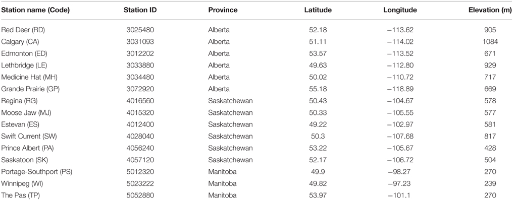
Table 1. Climate stations with location and elevation.

FIGURE 1

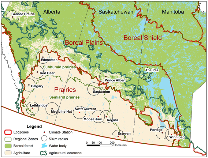
Figure 1. Climate station locations, Canadian ecozones, regional zones, agricultural regions, and boreal forest.

Climate Data Set

The hourly climate variables include air pressure (P), dry bulb temperature (T), relative humidity (RH), wind speed and direction, total opaque cloud amount, and total cloud amount. All stations except Moose Jaw and Regina have data for the height and amount of the lowest cloud layer. Observers also reported cloud amount and type by layers (MANOBS, 2013), but our primary stratification variable is total opaque cloud, because it can be related on daily timescales to the radiation driving the diurnal cycle.

We generated a file of daily means for total opaque cloud, OPAQ_m, T_m, RH_m, and windspeed, V_m, which will be used for sorting, and for radiation fits (Section Climatological Radiation Fits to Opaque Cloud). We have a file of daily total precipitation and daily snow depth. The time-base of the data is Local Standard Time (LST). Across these Prairie stations, LST is later than local solar time by time intervals ranging from 0.3 to 1.2 h, but we made no correction for this. Note that we will only stratify using daily mean values, so that all stratifications contain a large number of complete days with generally all 24-hourly values. Since occasional hourly data were missing, we kept a count of the number of measurement hours, MeasHr, of valid data for each day. We have filtered out all days for which MeasHr < 21. There are few missing hours of data in the first four decades, but this filter removes recent periods with only daytime data.

Diurnal Range Choices

As discussed in the introduction, there has been considerable discussion in recent years about the difference between DTR, T_x, and T_n derived from monthly means of hourly data, and the conventional monthly mean of daily values of DTR, T_x, and T_n (Zeng and Wang, 2012; Betts et al., 2014a; Wang and Zeng, 2014; Li et al., 2016). Betts et al. (2014a) showed that in winter, and even in summer under cloudy conditions, that stratification by opaque cloud shows substantial differences between DTR and DRH calculated by averaging daily ranges, and values found from the mean diurnal cycles derived by averaging the hourly data. We explored this (Section Radiatively Forced Diurnal Ranges and Mean Diurnal Ranges) and concluded that for conceptual purposes the “true” diurnal cycle, meaning that which is coupled to the diurnally varying radiation field, is found by first compositing the hourly data for groups of many days, and then determining the diurnal ranges from the composites. This is what we shall generally show in Figures, although we will show a few comparisons with the average of daily values of DTR, T_x and T_n in Sections Warm and Cold Climates and the Transition Between them and Monthly Climatology. Since we have some 250,000 days in this dataset, even detailed sub-stratifications have > 100 days in each bin and coarse stratifications may have > 5000 days in each bin.

Formally we will define diurnal ranges derived by averaging daily values as

$\begin{array}{rc}{\text{DTR}}_{\text{D}}={\text{T}}_{\text{xD}}-{\text{T}}_{\text{nD}}& \left(\mathrm{1a}\right)\hfill \end{array}$

$\begin{array}{rc}{\text{DRH}}_{\text{D}}={\text{RH}}_{\text{xD}}-{\text{RH}}_{\text{nD}}& \left(\mathrm{1b}\right)\hfill \end{array}$

and the “true” radiatively coupled diurnal ranges, derived by first averaging many days of hourly data and extracting the diurnal ranges from the composites, as

$\begin{array}{rc}{\text{DTR}}_{\text{T}}={\text{T}}_{\text{xT}}-{\text{T}}_{\text{nT}}& \left(\mathrm{2a}\right)\hfill \end{array}$

$\begin{array}{rc}{\text{DRH}}_{\text{T}}={\text{RH}}_{\text{xT}}-{\text{RH}}_{\text{nT}}& \left(\mathrm{2b}\right)\hfill \end{array}$

In the warm season, when surface heating couples with a daytime convective BL then typically RH reaches a maximum near sunrise at T_nT and a minimum at the time of the afternoon T_xT. We also derived from P, T, and RH, the mixing ratio (Q), the potential temperature (θ), the equivalent potential temperature (θ_E), and the saturation pressure (p*) at the lifting condensation level (LCL). Following Betts (2009), we defined the pressure height to the LCL, P_LCL = P − p*, which in the warm season is often an indicator of the height of cloud base (Betts et al., 2013a). We calculated the diurnal ranges: Dθ_ET and DP_LCLT.

If OPAQ_m < 0.7, mixing ratio Q has a morning and evening double peak in the warm season, and a sunrise and an afternoon minimum (see Section Mean Diurnal Cycles for the Three Regimes). Under more cloudy conditions, there is only a single peak. We calculated the morning diurnal range, DQ-am, as the rise to the first or only maximum, and for OPAQ_m < 0.7 we calculated the afternoon diurnal range, DQ-pm. Even T_nT and occasionally RH_xT have ambiguity under very cloudy conditions, when there is systematic cooling and moistening over the 24-h period, probably from the evaporation of falling rain (see Section Monthly Mean Diurnal Ranges and 24-h Imbalances for the Warm Season). Then it is possible that the temperature at LST = 23 h is below the previous morning minimum. We dealt with this by choosing T_nT and RH_xT for the hours from LST = 0 to 20 h. Note that the 24-h means, such as OPAQ_m and T_m, are not affected by the order of averaging. Our figures will use both Celsius and Kelvin units for temperature.

Climatological Radiation Fits to Opaque Cloud

We will relate the daily net longwave flux, LW_n (in W/m²), to OPAQ_m (as a fraction) using the Betts et al. (2015) fits derived using multiple linear regression between daily means of opaque cloud data at Regina and daily means of the BSRN data, partitioned by T <> 0°C. Their warm season (T > 0^oC) fit was (R² = 0.91)

$\begin{array}{cc}\begin{array}{l}{\text{LW}}_{\text{n}}=-128.6(\pm 7.8)+28.1(\pm 1.8){\text{OPAQ}}_{\text{m}}+44.6\hfill \\ (\pm 1.8){\text{OPAQ}}_{\text{m}}^2+0.49(\pm 0.01){\text{RH}}_{\text{m}}\hfill \end{array}& (3\text{a})\end{array}$

Their cold season fit (T < 0^oC) had a significant dependence on T_m, but a reduced dependence on RH_m and a lower R² = 0.83

$\begin{array}{cc}\begin{array}{l}{\text{LW}}_{\text{n}}=-89.2(\pm 10.1)+43.5(\pm 2.8){\text{OPAQ}}_{\text{m}}+26.8(\pm 2.5)\hfill \\ {\text{OPAQ}}_{\text{m}}^2+0.29(\pm 0.02){\text{RH}}_{\text{m}}-1.02(\pm 0.03){\text{T}}_{\text{m}}\hfill \end{array}& (3\text{b})\end{array}$

Following Betts and Viterbo (2005) and Betts (2009), we define an effective cloud albedo, ECA, as the scaled SWCF, the difference between the daily mean downward all-sky and clear-sky shortwave fluxes (SW_dn− SWC_dn) defined as

$\begin{array}{rc}\text{ECA}=-{\text{SWCF}∕\text{SWC}}_{\text{dn}}& \left(4\right)\hfill \end{array}$

For the downward clear-sky flux, we used the empirical fit, as a function of Day of Year (DOY), derived by comparing SWC_dn from the nearest grid point of the European Centre reanalysis, known as ERA-Interim, with the BSRN data on days with clear skies (Betts et al., 2015)

$\begin{array}{rc}{\text{SWC}}_{\text{dn}}=55+300^{*}\text{SIN}{(\pi \text{DS}∕365)}^{1.92}& \left(5\right)\hfill \end{array}$

where DS = DOY + 14 for DOY < 353, and DOY − 352 for DOY < 353. For the composites in this paper we will ignore leap years. The net shortwave flux is

$\begin{array}{rc}{\text{SW}}_{\text{n}}=(1-{\alpha }_{\text{s}}){\text{SW}}_{\text{dn}}=(1-{\alpha }_{\text{s}})(1-\text{ECA}){\text{SWC}}_{\text{dn}}& \left(6\right)\hfill \end{array}$

where we used representative values for the surface albedo, α_s, of 0.2 and 0.7 for a snow-free and snow-covered surfaces on the Prairies (Betts et al., 2014a). We compute net radiation, R_n, as

$\begin{array}{rc}{\text{R}}_{\text{n}}={\text{SW}}_{\text{n}}+{\text{LW}}_{\text{n}}& \left(7\right)\hfill \end{array}$

For the computation of ECA from OPAQ_m, we adapted fits derived in Betts et al. (2015): details are given in the Appendix. Note that we used fits from the BSRN site near Regina to interpret opaque cloud cover for all the climate stations. The next section addresses the consistency of the opaque cloud observations across the Prairies.

Evaluation of Opaque Cloud Data

Since we are using the opaque/reflective cloud data for stratification, we first assessed the quality of these cloud data made by trained observers across the Prairies for the past 60 years.

Close Neighbor Comparison of Opaque Cloud Data

Figure 2 compares daily mean opaque cloud for three neighboring pairs: Regina and Moose Jaw separated by 63 km, Winnipeg and Portage-Southport, separated by 75 km, and Regina, and Estevan, separated by 181 km. The geometric mean slope of the regression of y on x and x on y shown are close to unity, showing that these daily means estimated by independent observers appear to be unbiased, and that daily mean cloud data at one station is spatially representative for distances of order 100 km. This is not surprising as the 24 h advection distance at 3 m/s is 260 km.

FIGURE 2

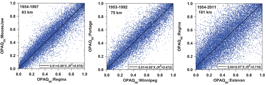
Figure 2. Comparison of daily mean opaque cloud cover for Moose Jaw and Regina for 1954–1997 (left); (center) Portage-Southport and Winnipeg for 1953–1992, and (right) Regina and Estevan for 1954–2011.

Figure 3 shows how the linear regression R²-values decrease as the distance increases between climate station pairs (identified by their 2-letter code in Table 1). The R²-values for daily mean OPAQ_m are systematically higher than for the daily solar weighted opaque cloud fraction, OPAQSW (see Appendix), which is computed from a smaller number of cloud values during daylight hours. The linear regression fits are shown. The points above the lines are on the Prairies in Saskatchewan and Manitoba; those below are in Alberta in the lee of the mountains, and Saskatoon paired with Prince Albert on the edge of the boreal forest. The geometric mean slopes of the opaque cloud regressions for each of these station pairs are close to unity out to the spacing of 250 km (not shown); so we shall treat these opaque cloud observations by independent observers as unbiased for this climatological analysis.

FIGURE 3

Figure 3. Decrease of correlation of daily opaque cloud with increasing station spacing.

Interannual Variability of Opaque Cloud

An independent check on the long-term quality of the opaque cloud data is the comparison of interannual variability across stations. Figure 4 shows the time-series of annual means grouped by provinces. The upper panels are a mean for the warm season months (April to October: AMJJASO) and the lower panels are a mean for the cold season months (November to March: NDJFM). For reference, each plot shows the 13-station mean (heavy magenta), excluding Swift Current, for which there is good data only for 1953–1979, and Edmonton, where the data is not available before 1961. There are interesting time variations in mean cloud cover across the Prairies in the 58-year period: a general warm season decline from 1953 to 1988 and a general increase from 1988 to 2010. During the warm season, the more northern stations (in blue) have generally more opaque cloud cover then the southern stations (in red). The cold season interannual variability appears larger than in the warm season. In general, the coherence between close station pairs, suggests that the observational protocol for the opaque cloud data has been maintained across the Prairies over the long time period. One clear exception is apparent: there is a discontinuous drop in the mean cloud cover at Lethbridge, starting in May 1994 and lasting many years; so we excluded these data from our analysis.

FIGURE 4

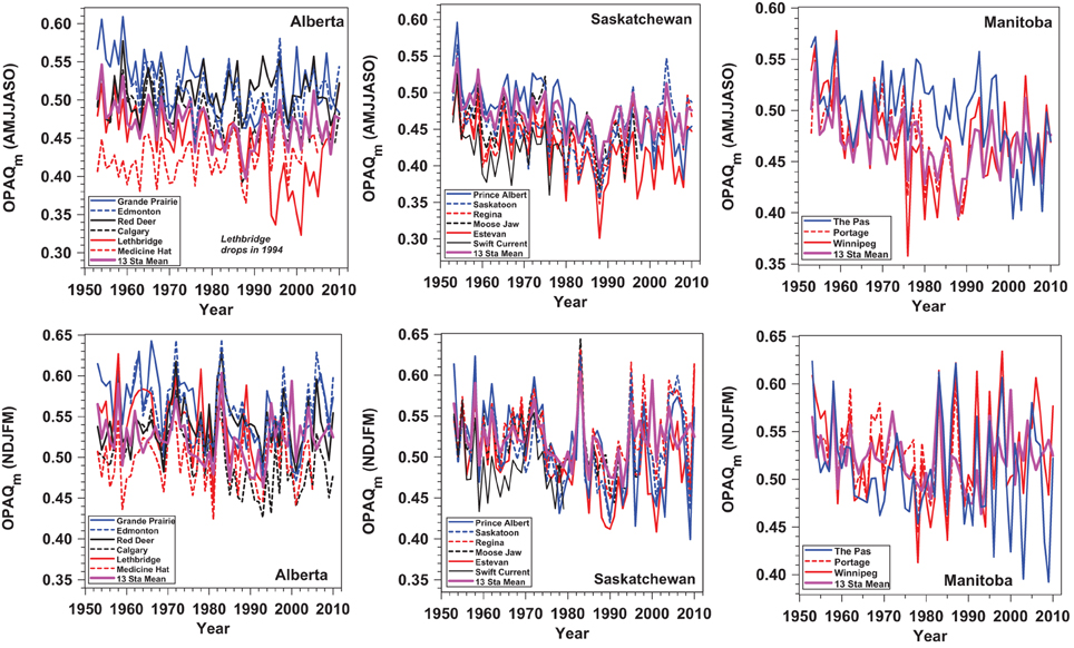
Figure 4. Variation of mean opaque cloud for warm (top) and (bottom) cold seasons, grouped by Provinces, together with a 13-station Prairie mean from 1953 to 2010.

There is much more variability in cloud cover between the stations close to the Rocky Mountains in Alberta, where the most northern station (Grande Prairie) has the most cloud cover, and Medicine Hat in the southeast is less cloudy in the early years. There is much less cloud variability between the six stations in Saskatchewan. For the years of data, 1953–1979, Swift Current has lower cloud cover than other stations in Saskatchewan; similar to Medicine Hat, 218 km to the west in Alberta. Clearly the regional and long-term variability is large and deserves further analysis. However, for the purpose of this paper we are merging the data across the Prairies to show the climatological coupling to opaque cloud, rather than the long-term trends.

Interannual Variability of Surface Radiation

To show how the cold and warm season climatologies differ, we estimated the long-term variability in the surface radiation balance over the Prairies from the monthly variability in OPAQ_m, OPAQSW, RH_m, and T_m, using Equations (3), (6), and (7). Figure 5 (left panels) show the annual variability of SW_n, LW_n, and R_n, as a mean for the seven warm (AMJJASO) and five cold (NDJFM) season months. In the warm season, SW_n and LW_n are anti-correlated because cloud cover reflects sunlight but reduces the LW cooling to space. However, SWCF dominates and as a result R_n has a damped response, increasing as cloud cover decreases. The remarkable long-term feature is the 1988 peak of SW_n, coming from the cloud minimum in Figure 4. Linear regression lines are shown for the periods, 1953–1988, and 1988–2010, to illustrate the reversal of the long-term linear trends in 1988. In contrast, for the cold season, LWCF >> (-SWCF) and the variability of R_n is dominated by LWCF, and we show the linear regression fits for the entire period. These long-term trends clearly need further analysis, but this is outside the scope of this paper, as it is likely that it involves the coupling of the Prairie climate to the Pacific and Arctic circulations.

FIGURE 5

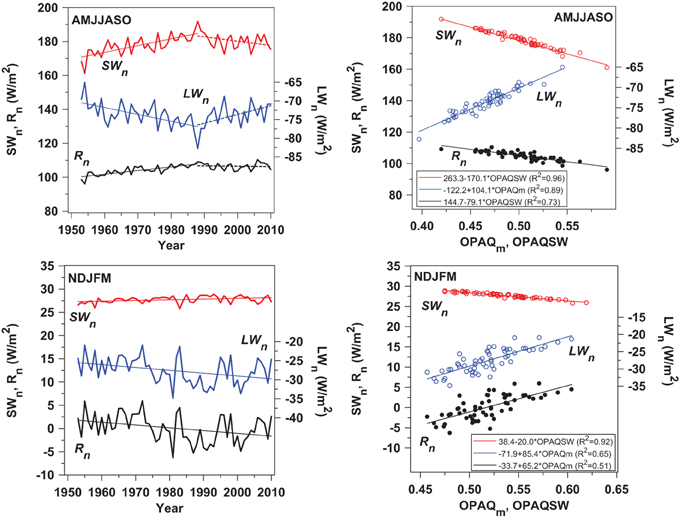
Figure 5. Interannual variability of SW_n, LW_n, and R_n for warm season (AMJJASO) and cold season (NDJFM) (left) and (right) regression of SW_n and R_n on OPAQSW, LW_n on OPAQ_m in warm season (top); SW_n on OPAQSW, LW_n and R_n on OPAQ_m in cold season (bottom).

The right panels show the relationship between the annual variability of opaque cloud and SW_n, LW_n, and R_n for these distinct warm and cold season regimes. We see that over this period of 58 years, the absolute ranges of (SW_n, LW_n, R_n) for increasing cloud are (−30.8, 17.7, −13.3 W/m²) for the warm season, and (−3.1, 13.9, 12.2 W/m²) in the cold season. Note that we have plotted SW_n against OPAQSW and LW_n against OPAQ_m, because that is how they are computed; but we plot R_n against OPAQSW in the warm season and against OPAQ_m in the cold season, because they are more highly correlated with the dominant term.

These fundamental differences between the warm and cold season radiative forcing by clouds, seen in Figure 5 (right panels) on the interannual scale, exist on the daily, and monthly timescales; where Betts et al. (2015) showed that LWCF dominates in the cold season and SWCF dominates in the warm season.

Annual Diurnal Cycles of Opaque Cloud

Figure 6 (top panels) shows the annual cycle of the diurnal cycle of total and lowest-level opaque cloud cover averaged across all stations in Table 1. Two stations (Moose Jaw and Regina) have no lowest-level cloud observations. It is clear that the warmest months, July, and August, have less cloud cover. This signature is seen in both the total and lowest-level cloud cover (upper panels). To remove the strong annual cycle and highlight the time of day of maximum and minimum cloud cover, each month is normalized and scaled by the range between its maximum and minimum cloud cover, so that the scaled minimum and maximum are zero and one (lower panels).

FIGURE 6

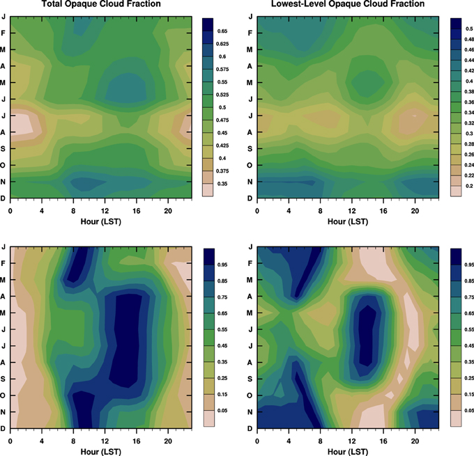
Figure 6. The average diurnal cycle of total opaque cloud fraction and lowest-level opaque cloud fraction over the annual cycle (top), and (below) the normalized diurnal cycles of total opaque cloud cover fraction and lowest-level opaque cloud fraction, scaled so that 1 is the diurnal maximum and 0 is the minimum.

This shows a clear shift in the time of day of maximum opaque cloud cover between cold and warm seasons. There is a morning (6 to 9 LST) maximum in total opaque cloud from November through March, and an afternoon (14 to 16 LST) maximum during the warm months, May through September (lower left). April and October are transition months. This separation of these diurnal maxima is sharper in the lowest-level cloud field (lower right). The morning maximum in low cloud, which is dominant in the cold season, is close to or a little before the minimum temperature near sunrise, and varies seasonally. The warm season afternoon low cloud maximum is about an hour ahead of the afternoon temperature maximum at 15 LST (see next section). Betts et al. (2014a, 2015) identified a sharp warm/cold regime change, which they attributed to a “fast” radiative switch corresponding to whether snow was present on the ground. However, we see that for the transition month of October, which is before significant snowfall at many stations, the morning and afternoon maxima in total opaque cloud are both present (bottom left). However, the afternoon maximum of low cloud found from April to September is no longer present (bottom right).

Warm and Cold Climates and the Transition Between Them

There are two primary Prairie climates, sharply separated by the freezing point of water: one for the cold season with surface snow cover, and one for the warm season without snow. This is because surface snow acts as a climate switch (Betts et al., 2014a) that changes the sign of the net cloud radiative forcing (Betts et al., 2015).

Mean Diurnal Cycles for the Three Regimes

Figure 7 shows the stratification by daily mean opaque cloud (OPAQ_m) for these two regimes and the much smaller mixed class, when it is below freezing but there is no snow cover, or it is above freezing but not all the snow has melted. The very large size of these datasets means that the standard error (SE) of the means, shown only for the extremes of cloud cover, are very small.

FIGURE 7

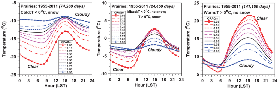
Figure 7. Diurnal cycle of temperature stratified by OPAQ_m for cold season with snow cover, mixed regime and warm season without snow cover.

For the cold-snow class (74,260 days), the average snow depth and windspeed across the 10 cloud groups are 17.2(±0.7) cm and 3.69(±0.17) m/s, respectively. T_nT at sunrise (and T_m) fall as cloud cover decreases. This is characteristic of a stable BL that is LWCF dominated (Betts et al., 2015), where temperatures are warmest under cloudy skies, and fall to a very low minimum around sunrise under nearly clear skies. Under the same clear skies, the diurnal cycle of temperature driven by the daytime solar forcing is largest. For the warm-no-snow class (142,160 days, mean windspeed of 3.85(±0.31) m/s), T_nT at sunrise barely changes, but afternoon T_xT (and T_m) increase as cloud cover decreases. This warm regime is SWCF dominated, characterized by a growing unstable convective BL in the daytime (Betts et al., 2015), and the coolest temperatures under cloudy skies, when 69% of the days have > 1 mm of precipitation. The mixed regime (24,450 days) appears to be a blend with a more symmetric diurnal rise and fall about a mean temperature a little below freezing. However, closer inspection shows that as OPAQ_m falls from 0.95 to 0.65, T_xT rises, but as cloud cover is reduced further, the diurnal range is increased due to a cooling in T_nT. Across the 10 cloud bins, the mean windspeed is 3.97(±0.25) m/s, and average snow depth is only 3.3(±0.8) cm.

Figure 8 shows RH and P_LCL for the three regimes. The amplitudes of the diurnal patterns increase with decreasing opaque cloud, and there is a large increase in the nearly clear sky diurnal amplitude from cold to warm regimes. The top and bottom rows are nearly mirror opposites, because RH largely determines the LCL with only a small temperature dependence (Betts, 2009). For the cold regime (T < 0°C with surface snow), the variation of both RH and P_LCL with cloud cover is small. The warm regime shows a strong diurnal cycle with a minimum in RH and maximum of P_LCL in the afternoon at the temperature maximum. The mixed regime near freezing again lies in-between. For the warm and cold regimes, the SE-values for RH- are < 0.2% and for P_LCL < 0.5 hPa: tiny compared with the variation with opaque cloud cover.

FIGURE 8

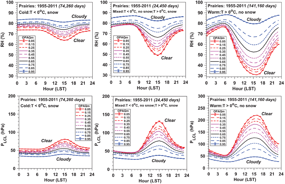
Figure 8. As Figure 7 for RH and P_LCL.

The diurnal cycle of mixing ratio, Q, has marked structural differences across the three regimes (Figure 9). The cold regime with snow and the mixed regime have a diurnal cycle with a single afternoon peak near the time of maximum temperature. However, the warm regime for OPAQ_m < 0.7 shows morning and evening peaks in Q with local mid-afternoon and pre-sunrise minima. This is the characteristic signal of an unstable growing daytime BL, which couples and uncouples to a deeper BL above (Betts et al. (2013a). After sunrise, evaporation is trapped for some hours in the shallow night-time BL, warming and moistening the near-surface air after the sunrise minimum. Around 10 LST, the growing BL recouples with a deep residual BL, and Q falls to an afternoon minimum as the growing BL entrains drier air from above. After the time of maximum temperature, the near-surface layer again decouples, and Q rises until sunset when evapotranspiration drops to very low values. In Section Monthly Mean Diurnal Ranges and 24-h Imbalances for the Warm Season, we will compute the morning (DQ-am) and afternoon (DQ-pm) diurnal ranges for OPAQ_m < 0.7 from the warm season monthly data.

FIGURE 9

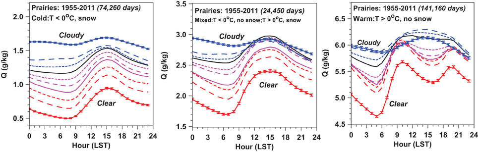
Figure 9. As Figure 7 for mixing ratio, Q.

Conserved Variable Diagrams

Conserved variable diagrams show a useful summary of the coupled diurnal cycle of all the thermodynamic variables (Betts, 1982, 2009). Figure 10 remaps the warm-no snow and cold-snow composites from Figures 7–9 onto a conserved variable (θ, Q) plot. We show just three composites, corresponding to OPAQ_m = 0.05, 0.45, and 0.85. We have added the saturation pressure lines, p*, and (left panel) also the lines of constant θ_E at saturation to show how the diurnal cycle of saturation level (LCL) and surface θ_E are also represented on this saturation point diagram. The mean surface pressure is close to the 940 hPa isopleth shown. The hour numbers show the time sequence of the diurnal cycle. For example for the warm season nearly-clear sky composite (left panel), we see the early morning cooling from 0 LST to the 5 LST minimum, the rise to the Q maximum at 10 LST, followed by the rise of θ and fall of Q as the maximum temperature is approached. The downward return path shows the evening Q maximum at 20 LST. In contrast the cold season composite (right panel) shows the diurnal warming and moistening, but it has very little range in saturation pressure.

FIGURE 10

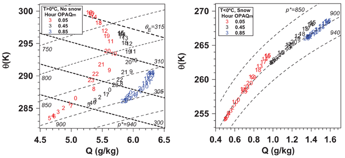
Figure 10. Conserved variable plot for (left) warm season without snow and (right) cold seaason with snow for OPAQm = 0.05, 0.45, and 0.85.

Non-Stationarity of the Diurnal Cycle

The diurnal cycle composites in Figure 10 sorted by opaque cloud come from a very large dataset. The number of days in the three warm season composites for OPAQ_m of 0.05, 0.45, and 0.85 are 14260, 17800, and 8200, respectively. However, the mean diurnal cycle is not in an equilibrium state. In the left panel of Figure 10 for OPAQ_m = 0.05, close inspection shows a non-uniform sequence for the hours 22, 23, 0, and 1. The data for hour = 23 at the end of the day is noticeably warmer and a little moister than the simple backward extrapolation from hour 1 to 0, giving a significant discontinuity across local midnight. Figure 11 shows these 24-h imbalances of T, RH, and Q, as a function of OPAQ_m, calculated as

$\begin{array}{rc}{\text{ΔT}}_{24}=({\text{T}}_{23}-{\text{T}}_0)+0.5^{*}({\text{T}}_1-{\text{T}}_0+{\text{T}}_{23}-{\text{T}}_{22})& \left(\mathrm{8a}\right)\hfill \end{array}$

$\begin{array}{cc}\begin{array}{l}\Delta {\text{RH}}_{24}=({\text{RH}}_{23}-{\text{RH}}_0)+{0.5}^{\ast }({\text{RH}}_1-{\text{RH}}_0+{\text{RH}}_{23}\hfill \\ -{\text{RH}}_{22})\hfill \end{array}& (8\text{b})\end{array}$

$\begin{array}{c}\Delta {\text{Q}}_{24}=({\text{Q}}_{23}-{\text{Q}}_0)+{0.5}^{\ast }({\text{Q}}_1-{\text{Q}}_0+{\text{Q}}_{23}-{\text{Q}}_{22})(8\text{c})\end{array}$

FIGURE 11

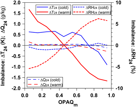
Figure 11. Twenty-four hours imbalance of T, RH, and Q for warm and cold composites.

For temperature, the first term is the difference between the beginning and end of a diurnal composite, and the second is the average of the hourly cooling at the beginning and end of each composite. ΔT₂₄ is zero if these cancel. However, we see that for the warm season composite over the range of OPAQ_m from 0.05 to 0.95, (ΔT₂₄, ΔRH₂₄, ΔQ₂₄) change from (+1.7 K, −5.4%, 0.16 g/kg) to (−1.7 K, +5.8%, −0.28 g/kg). For the cold season composite with snow, the imbalances are smaller. For the warm season hourly means, the SE for T ≈ 0.05 K and for RH ≈ 0.15%, more than an order of magnitude smaller than the T and RH imbalances in Figure 11. In Section Monthly Mean Diurnal Ranges and 24-h Imbalances for the Warm Season, we will discuss further this warm season warming and drying under nearly clear skies, and cooling and moistening under cloudy skies with rain, using the monthly data.

Radiatively Forced Diurnal Ranges and Mean Diurnal Ranges

As discussed in Section Diurnal Range Choices, there are important differences between DTR_T and DTR_D. Wang and Zeng (2014) noticed that DTR_D, the monthly mean of daily DTR, was greater than DTR_T, calculated from the monthly mean diurnal cycle, especially at high latitudes and in winter. Betts et al. (2014a) found similar differences using summer and winter cloud stratifications using the Prairie data. The differences between these two methods of averaging are large and conceptually important. Figure 12 shows the OPAQ_m stratification of T_x, T_n and DTR (left) and RH_x, RH_n, DRH, and daily precipitation (right) for the warm-no-snow (top) and cold-snow (bottom) composites, which contain 141160 and 74260 days respectively. The solid lines, labeled T, come from the composites in Figures 7, 8, while the dashed lines come from calculating the corresponding mean of the daily values for the same variables for the same data stratification.

FIGURE 12

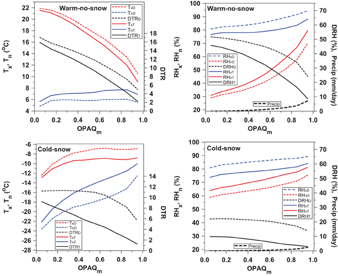
Figure 12. T_x, T_n, and DTR (left) and RH_x, RH_n, DRH and daily precipitation (right) for the warm-no-snow (top) and cold-snow (bottom). Solid lines come from Figures 7, 8, while the dashed lines are the corresponding means of the daily values.

We see a systematic bias with (T_xD, RH_xD) > (T_xT, RH_xT) while (T_nD, RH_nD) < (T_nT, RH_nT). These biases arise because after averaging T_nT and T_xT (and typically RH_xT and RH_nT) are tied to the solar cycle, specifically the sunrise temperature minimum and the peak solar heating temperature maximum typically in the afternoon. However, given daily advective processes, T_nD can be at any time, and will by definition be equal to or colder than the sunrise temperature. Similarly T_xD is necessarily equal to or warmer than the early afternoon temperature. The result of these biases is that the true radiatively coupled (DTR_T, DRH_T) < (DTR_D, DRH_D). This bias in the diurnal ranges is largest for the cloudy and winter composites that have the smallest diurnal radiative forcing. As in Figures 7, 8, the very large size of these datasets means that the SE of the means are ≤ 0.1 K for T and < 0.2% for RH in both warm and cold seasons (not shown).

DTR_T is almost linearly related to OPAQ_m for both warm and cold composites, and DTR_T and DRH_T drop to near zero, when extrapolated to 100% opaque cloud conditions, in sharp contrast to DTR_D and DRH_D. The mixed regime composite (not shown) has similar systematic differences, as do the monthly composites which we will show in the next section. Note that for OPAQ_m = 0.95, mean daily precipitation for the warm and cold classes reaches 7.11 and 2.35 mm/day, but for OPAQ_m = 0.55 it is only 1.1 mm/day for the warm class.

Much of our long-term climatological data records daily T_xD and T_nD from which DTR_D = T_xD−T_nD and T_mD = (T_xD + T_nD)/2 are derived. We see from Figure 12 that the climatological bias of this estimate of T_mD may be less than for DTR_D; even though it is still not the true diurnal mean, which in this analysis is an average of 24 hourly values.

Monthly Climatology

Monthly Diurnal Cycle for Warm-No-Snow; Cold-Snow Classes

Figure 13 shows the diurnal cycle by month with the sub-division into the two main classes: cold season with snow cover and warm season without snow cover. May to October show the warm season increase of T_x with decreasing cloud, while December to February show the cold season strong decrease of T_n with decreasing cloud. For the months showing only a single warm or cold class, there are more than 1000 days in each cloud bin. Only March, April, and November have enough data (> 200 days per cloud class) to show all cloud bins for both cold and warm regimes. These months clearly show the role of snow cover as a climate switch. There is a clear regime separation with T_m above and below the dashed freezing line (note the much larger T-axis range). The impact of snow cover on the climatology is a cooling of the order of 10 K, as noted in Betts et al. (2014a). We will discuss the cold season, the transition months and the warm season separately in Sections Cold Season with Snow, Snow Transition Months, and Monthly mean Diurnal Ranges and 24-h Imbalances for the Warm Season. We do not show the small SE of these binned monthly means: for the warm-no-snow bins, the SE for T ≈ 0.1 K, and for the cold-snow data, the SE for T ≤ 0.3 K.

FIGURE 13

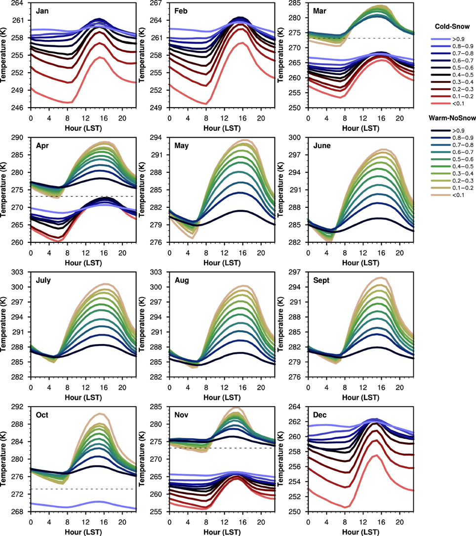
Figure 13. Monthly diurnal cycles for cold-snow and warm-no-snow classes, stratified by OPAQ_m.

Cold Season with Snow

Figure 14 (left panel) shows the relation between OPAQ_m, T_m, and R_n for the cold season months, November to March, selecting only those days with T_m < 0°C and snow cover. Monthly mean T_m increases with cloud cover, because LWCF dominates in the cold months with surface snow (Figure 5). The seasonal cycle of T_m has a minimum in January, 1 month after the minimum of R_n.

FIGURE 14

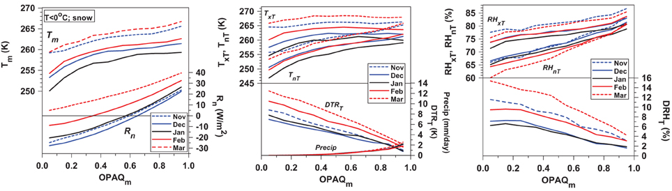
Figure 14. Monthly T_m and R_n (left); (center) T_xT, T_nT, DTR_T, and precipitation; and (right) RH_xT, RH_nT, DRH_T as a function of OPAQ_m.

The center panel shows that the DTR_T derived from T_xT and T_nT in Figure 13 has a quasi-linear increase with decreasing cloud. The typical cold season SE for T_xT and T_nT ≤ 0.3 K (not shown). DTR_T has a minimum in December with the minimum in the solar elevation angle, and increases from December to March as SW_n increases. Multiple linear regression of DTR_T on OPAQ_m and SW_n gives an excellent fit (R² = 0.98)

$\begin{array}{cc}\begin{array}{l}{\text{DTR}}_{\text{T}}=5.7(\pm 0.4)-6.7(\pm 0.2){\text{OPAQ}}_{\text{m}}\hfill \\ +0.116(\pm 0.005){\text{SW}}_{\text{n}}\hfill \end{array}& (9)\end{array}$

The upper lines show T_xT,above T_nT (Figure 14 middle panel). As OPAQ_m falls, the minimum temperatures fall more steeply than the maximum temperatures. There is also a seasonal change: by March, T_xT is almost independent of OPAQ_m, and the fall of T_nT with decreasing OPAQ_m has become nearly linear. Daily mean precipitation increases with OPAQ_m but the monthly dependence is small. Mean wind speed increases only about 15% with increasing cloud cover (not shown) and the mean across the five cold season months is = 3.68(±0.08) m/s.

The right panel shows the corresponding RH plots, for which the typical SE for RH_xt and RH_nT ≤ 0.5% (not shown). The increase of DRH_T with decreasing cloud shows a similar but not identical pattern to DTR_T over the winter season. RH_xT is largest in November. The time of the RH maximum in winter under clearer skies is often well before sunrise (not shown), perhaps because RH falls with surface ice deposition as the surface cools.

Snow Transition Months

Figure 15 shows the climatological impact of snow as a function of opaque cloud cover for November and for March, the two transition months with the most data in both classes. The left panel shows T_xT, T_m, and T_nT from Figure 13 for the warm-no-snow class (upper group) and the cold-snow class (lower group). The two groups separate cleanly, and show very distinct structures. Both have a diurnal range, larger in March than in November. However, for the warm group, T_xT increases and T_nT decreases as OPAQ_m falls; while for the cold group, T_xT is relatively flat, but T_nT falls steeply with decreasing cloud. The freezing point of water is shown for reference.

FIGURE 15

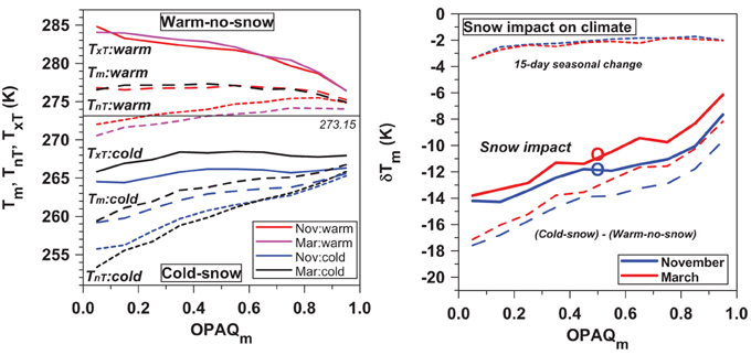
Figure 15. T_xT, T_m and T_nT (left), and (right) T_m differences between cold-snow and warm-no-snow classes for November and March as a function of opaque cloud cover. Month color scheme legend (left) is for T_xT.

The right panel shows the impact on the local climate. The lower dashed lines are the simple differences of T_m from the left panel between snow–no-snow classes as a function of opaque cloud; showing that the differences become larger as OPAQ_m decreases. We made a small correction for the general seasonal trend over 15 days as a function of OPAQ_m (dotted lines), because in general the days with snow are later in November and earlier in March. For November, we used the mean of the warm-no-snow gradient between October and November and the cold-snow gradient between November and December, which were similar. For March we used the same procedure, with similar results. Subtracting these estimates of the 15-day seasonal change gives an estimate of the climatological impact of the snow (solid lines). Not surprisingly we see the cooling increases from −7 to −14 K as OPAQ_m falls, because of the impact of the higher albedo of snow on SW_n (Betts et al., 2014a). The mean cooling across all cloud covers (heavy circles) for (November, March) are (−11.8, −10.7 K). These values for the climatology are very similar to those shown in Tables 2, 3 of Betts et al. (2014a) which were derived by compositing the transitions in time across snowfall in the fall, and snowmelt in the spring. The corresponding plots for T_xT and T_nT differences are very similar (not shown), with slightly larger differences for T_xT and slightly smaller ones for T_nT.

Monthly Mean Diurnal Ranges and 24-h Imbalances for the Warm Season

Figure 16 (left panel) shows the mean diurnal ranges of temperature, DTR_T, relative humidity, DRH_T, and mean daily precipitation for the warm season months April to September with no snow. The diurnal ranges are tightly clustered, as noted in Betts et al. (2013a), so we show the 6-month warm season mean (MeanT). We also show the corresponding MeanD, the 6-month average of all the daily values of DTR_D and DRH_D, which are similar to those shown in Figure 12 (upper panels), for the larger dataset. DTR_T and DRH_T for October (not shown) fall below MeanT by about 0.9°C and 4.3%, and we excluded October from this warm season group. The quadratic regression fits for the dependence of the 6-month mean DTR_T and DRH_T on OPAQ_m are

$\begin{array}{cc}\begin{array}{l}{\text{DTR}}_{\text{T}}=16.7(\pm 0.4)-9.3(\pm 0.8)\ast {\text{OPAQ}}_{\text{m}}\\ -6.0(\pm 0.7)\ast {\text{OPAQ}}_{\text{m}}^2(R^2=0.992)\end{array}& (10\text{a})\end{array}$

$\begin{array}{cc}\begin{array}{l}{\text{DRH}}_{\text{T}}=47.5(\pm 0.8)-2.6(\pm 1.4)\ast {\text{OPAQ}}_{\text{m}}\\ -38.9(\pm 1.4)\ast {\text{OPAQ}}_{\text{m}}^2(R^2=0.996)\end{array}& (10\text{b})\end{array}$

FIGURE 16

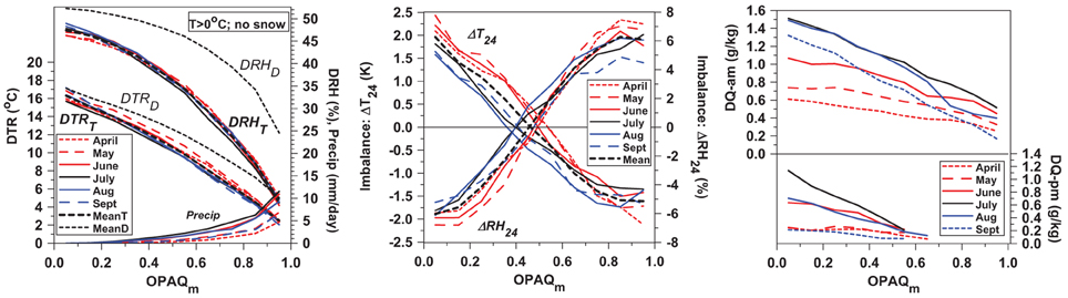
Figure 16. OPAQ_m dependence of DTR, DRH and precipitation (left) and (center) 24-h imbalances of ΔT₂₄and ΔRH₂₄, and (right) morning and afternoon rise of Q for April to September.

For OPAQ_m = 1, these fits have the values (DTR_T, DRH_T) = (1.4, 6.0). The increase of precipitation with OPAQ_m is largest in summer, peaking in July when T and Q peak (see also right panel discussed below). However, mean June precipitation (2.28 mm/day) is greater than July (1.91 mm/day) because June has substantially greater opaque cloud cover (Betts et al., 2014b).

The diurnal composites have a significant discontinuity across local midnight that depends on opaque cloud cover, which we discussed in Section Radiatively Forced Diurnal Ranges and Mean Diurnal Ranges. We calculated the 24-h imbalances ΔT₂₄ and ΔRH₂₄ from Equations (8a) and (8b), and these are shown in Figure 16 (center panel). We see that as OPAQ_m changes from 0.05 to 0.95, the mean (ΔT₂₄, ΔRH₂₄) change monotonically from (+2 K, −6%) to (−1.5 K, +6%). Under nearly clear skies, the warming and drying over the diurnal cycle are slightly larger in April, May, and June as mean temperature is increasing, and slightly smaller in August and September. The SE of the hourly binned data from which Figure 16 is derived is ≈0.1 K for T, ≤ 0.5% for RH, and ≈0.05 g/kg for Q

Betts and Chiu (2010) noted in the discussion of their equilibrium model for the non-precipitating convective BL over land that this diurnal warming over the 24 h cycle needed to be quantified, as it was likely to be of the same order as the net radiative cooling of the BL. We see under nearly clear skies, a warming of +2°C and a drying of −6% over the diurnal cycle. This is about 12% of both DTR and DRH. At the other limit under cloudy skies, typically with rain, the cooling of −1.5°C and moistening of +6% may be partly driven by both the evaporation of rain and downdraft transports. Between these limits, there is a uniform progression with increasing cloud, and for the 6-month mean, ΔT₂₄ and ΔRH₂₄ cross zero for OPAQ_m = 0.45.

The warm season mixing ratio. Q, has a double peak (see Figure 9) for OPAQ_m ≤ 0.65. For each month, April to September, we computed the diurnal range from the morning minimum, typically at the time of sunrise, to the first maximum (DQ-am), which is in the late morning for OPAQ_m < 0.7, and then shifts to the mid-afternoon. For OPAQ_m < 0.7, we also computed the afternoon diurnal range (DQ-pm) from the mid-afternoon Q minimum to the near-sunset maximum. Figure 16 (right panel) shows DQ-am and DQ-pm. There is a clear seasonal cycle, with DQ-am having a maximum amplitude in July and August, and DQ-pm having a maximum amplitude in July, the peak of the seasonal cycle of T and Q (Betts et al., 2014b). Clearly this is also related to evaporation reaching a maximum at the peak of the growing season in July. In all months, DQ-am > DQ-pm, presumably because in the morning, evaporation is trapped in shallower BL. The morning rise of Q also includes the evaporation of dew.

Figure 17 shows the warm season diurnal ranges and 24-h imbalances for θ_ET and P_LCLT. As in the left two panels of Figure 16, the diurnal ranges and the diurnal imbalances have only a small spread from April to September. The quadratic fits for the OPAQ_m dependence of the 6-month means are

$\begin{array}{cc}\begin{array}{l}\text{D}{\theta }_{\text{ET}}=19.7(\pm 0.7)-9.4(\pm 1.2)\ast {\text{OPAQ}}_{\text{m}}\hfill \\ -7.5(\pm 1.2)\ast {\text{OPAQ}}_{\text{m}}^2(R^2=0.983)\hfill \end{array}& (11\text{a)}\end{array}$

$\begin{array}{cc}\begin{array}{l}{\text{DP}}_{\text{LCLT}}=181.4(\pm 4.9)-90.3(\pm 9.0)\ast {\text{OPAQ}}_{\text{m}}\hfill \\ -81.1(\pm 8.7)\ast {\text{OPAQ}}_{\text{m}}^2(R^2=0.991)\hfill \end{array}& (11\text{b)}\end{array}$

FIGURE 17

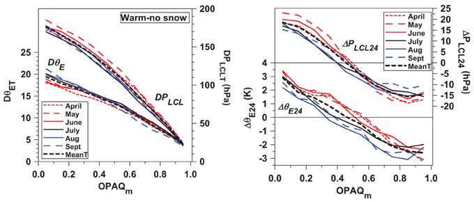
Figure 17. OPAQ_m dependence of Dθ_ET and DP_LCLT (left) and (right) 24-h imbalances of Δθ_E24and ΔP_LCL24 for April to September.

For OPAQ_m = 1, these fits have the values (Dθ_ET, DP_LCLT) = (2.73, 10.0).

Under nearly-clear skies, the mean 24-h imbalances show an increase of +2.9 K for θ_E and +18.6 hPa for P_LCL, which are 14.9% and 10.5% of the respective diurnal ranges. There is a corresponding small 24-h imbalance of mixing ratio of +0.2 g/kg. Under the other limit under nearly-overcast skies, typically with rain, the 24-h imbalance is a fall of -2.6 K for θ_E and -14.6 hPa for P_LCL, with a corresponding fall of Q of −0.24 g/kg. Figure 17 is derived from the hourly binned data, for which the warm season SE is ≤ 0.3 K for θ_E and ≤ 1.5 hPa for P_LCL.

Warm Season Conserved Variable Diagrams

We still lack a satisfactory theory for the remarkable homogeneity from April to September (noted in Betts et al., 2013a) of the diurnal ranges shown in Figures 16, 17 (left panels). They seem independent of the seasonal cycle of temperature and solar forcing, as well as the large seasonal cycle of evaporative fraction associated with the vegetation phenology. The conserved variable plots of the monthly climatology, shown in Figure 18, are a useful summary of the warm season climatology in graphical format. Because the diurnal ranges, DTR_T, DRH_T, Dθ_ET, and DP_LCLT vary little from April to September, the differences in Figure 18 come primarily from the substantial differences in DQ-am and DQ-pm in Figure 16. The large values of DQ-am are clearly visible in July and August for OPAQ_m = 0.05, as is the large July value of DQ-pm. The higher LCL (p* < 700 hPa) in May comes from the larger DP_LCL in Figure 17 and drier conditions at sunrise. A deeper analysis of the near-surface diurnal cycle of this fully coupled surface-BL-cloud system needs upper air data for the properties of the air entrained into the growing BL (Santanello et al., 2013), and estimates of the surface energy partition.

FIGURE 18

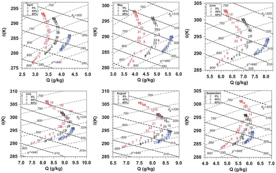
Figure 18. As Figure 10 for warm season composites from April to September.

Monthly Radiative-DTR Coupling

Figure 19 plots the diurnal temperature range against the surface radiation for the months April to September (left panels) and the winter months November to March with snow cover (right). The top panels show the monotonic dependence of DTR on LW_n, calculated from OPAQ_m using Equation (3). For DTR_T in the warm season (top-left), the 6 months are almost on top of each other, and we have overlaid the 6-month MeanT and the almost indistinguishable quadratic fit to this mean (R² = 0.999), which is of order zero for LW_n = 0.

$\begin{array}{cc}\begin{array}{l}{\text{DTR}}_{\text{T}}=0.1(\pm 0.1)-0.108(\pm 0.006){\text{LW}}_{\text{n}}\hfill \\ +0.00049(\pm 0.00005){\text{LW}}_{\text{n}}^2\hfill \end{array}& (12)\end{array}$

We also show the warm season linear dependence of DTR_D, the corresponding 6-month mean of the daily values, on LW_n and the linear fit (R² = 0.998)

$\begin{array}{rc}{\text{DTR}}_{\text{D}}=2.1(\pm 0.1)-0.145(\pm 0.002){\text{LW}}_{\text{n}}& \left(13\right)\hfill \end{array}$

Equation (13) agrees within the uncertainty with the linear fit derived using daily data for June, July, and August by Betts et al. (2015). It is consistent with the linear relationship found in model data (Betts, 2006), who suggested that this dependence of DTR on LW_n could be interpreted as the LW cooling from afternoon T_x to T_n the next morning. The (ECA, DTR_T) plot (bottom-left), where ECA comes from Equation (A2a) in the Appendix, is similar to the (LW_n, DTR_T) plot except that the spread between the 6 months is a little wider. This can be interpreted as the dependence of the DTR on the daytime SW warming from T_n to T_x. However, this relatively tight dependence on ECA, rather than SW_n or R_n, which both vary substantially from April to September, suggests that the daytime seasonal coupling has complex compensating processes. R_n is partitioned into sensible and latent heat fluxes (and ground storage), and this partition depends seasonally on both crop and natural vegetation phenology as well as soil moisture, for which we have no detailed information. In addition the daytime convective BL has a large growth from morning to mid-afternoon, which is coupled to the rise of 2-m temperature.

FIGURE 19

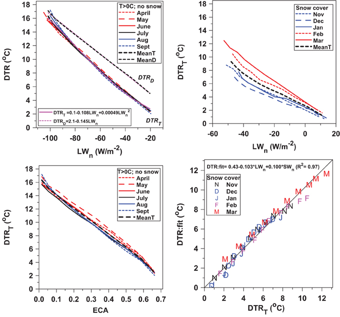
Figure 19. Warm season dependence of DTR_T and DTR_D on LW_n (top-left) and ECA (bottom-left); cold season dependence of DTR on LW_n (top-right) and (bottom-right) cold season regression fit to LW_n and SW_n.

In the cold season months with snow (top right), DTR_T increases with increasing outgoing LW_n, but it also has a SW_n dependence with a minimum in December, increasing to a maximum in March. Multiple linear regression gives the fit (R² = 0.97), shown in the bottom-right panel

$\begin{array}{cc}\begin{array}{l}\text{DTR}:\text{fit}=0.4(\pm 0.5)-0.103(\pm 0.004){\text{LW}}_{\text{n}}\\ +0.100(\pm 0.006){\text{SW}}_{\text{n}}\end{array}& (14)\end{array}$

This contrasts with Equation (12) for the warm season months April to September, where LW_n explains all the variance.

Stratification By Windspeed

Betts et al. (2015) showed the impact of daily mean windspeed on the mean summer (JJA) climate. We now revisit their analysis over the annual cycle using the full diurnal cycle data.

Cold Season with Snow

Figure 20 shows T_xT, T_nT, DTR_T, and precipitation as a function of OPAQ_m partitioned into four classes of daily mean windspeed (< 2, 2–4, 4–6, and >6 m/s) for the months December to March with snow cover. For each wind-class, we show the mean windspeed and the mean number of days for the 10 OPAQ_m bins. In all months there are fewer days in the highest windspeed category. DTR_T, which has a quasi-linear dependence on OPAQ_m, decreases as windspeed increases for all months, and for each wind-class, DTR_T increases from December to March, consistent with Figure 14. The increase of DTR_T with falling windspeed is not linear. Under nearly clear skies the difference between our low and high speed wind classes increases from 3.1°C in December to 5.2°C in March. For OPAQ_m > 0.55, precipitation and windspeed increase together, probably because major precipitation events are associated with higher winds.

FIGURE 20

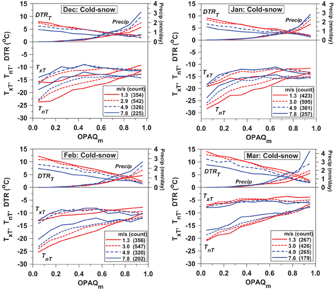
Figure 20. T_x, T_n, DTR, and precipitation as a function of OPAQ_m partitioned into four classes of daily mean windspeed, < 2, 2–4, 4–6, and >6 m/s, for the months December to March.

We see a cooling of T_nT with decreasing cloud and decreasing windspeed in all months that we could attribute to a strengthening of the stable BL, driven by LW cooling as windspeed and turbulent mixing both decrease. For OPAQ_m < 0.5, the mean fall of T_nT as windspeed falls is −6°C in December and January, but only −3.4°C in March.

However, there are interesting T_xT and T_nT pattern changes as the solar forcing increases from December to March. In December, and January, when the SW_n is small, both T_xT and T_nT fall with decreasing windspeed, most steeply under nearly clear skies as in Figure 14. By March, the drop of T_nT with windspeed is reduced, while T_xT shows a tendency to increase with windspeed, and these changes together maintain the larger spread of DTR_T. In addition, the March dependence on OPAQ_m has become more quasi-linear (as in Figure 14), with a larger negative slope for T_nT then T_xT. Although the mid-winter BL is dominated by LWCF (Betts et al., 2015), Equation (14) shows the dependence of DTR_T on both LW_n and SW_n. By March, both SW_n and SWCF have increased, but a detailed understanding of the windspeed dependence of this fully coupled system will need more study and modeling.

Warm Season with No Snow

Figure 21 shows the components of the diurnal cycle of temperature, θ_ExT and daily precipitation for the months April to September as a function of OPAQ_m and windspeed. In all months there is a similar non-linear decrease of DTR_T with increasing windspeed. There is a fall of T_nT (and rise of RH_xT, not shown) at low windspeeds and low cloud cover, which is −3.9 K for OPAQ_m < 0.2 in May and June, but only −1.9 K for July and August. This is perhaps because a more humid atmosphere reduces the LW cooling at night. This reduced cooling of T_nT is coupled to a small July-August warming of T_xT with decreasing windspeed. Combined with small increases of RH_nT (not shown), there is a July and August increase of afternoon θ_ExT of 4.4 K, averaged across all OPAQ_m, as windspeed decreases across the range shown (seen in (Betts et al., 2015) for summer). However, this increase of afternoon θ_ExT is much less in other months.

FIGURE 21

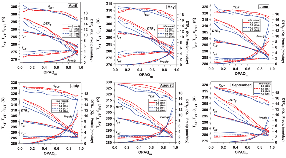
Figure 21. T_xt, T_nt, θ_Ext, DTR, and precipitation as a function of OPAQ_m partitioned into four classes of daily mean windspeed, <2, 2–4, 4–6, and >6 m/s, for the months April to September.

An increase of maximum θ_E in summer suggests that there may be increased moist convective instability at low windspeeds at the peak of the growing season (De Ridder, 1997). Comparing the wind dependence of θ_Ex and precipitation with increasing cloud cover, we see that for June, July and August, there is an indication that lower windpeed, higher θ_Ex and precipitation are coupled for OPAQ_m < 0.8. However, for all months for OPAQ_m = 0.95, there is a sharp increase of precipitation with windspeed, probably because the major rain events are associated with higher wind speeds. These results are consistent with the wind dependence shown in summer in Betts et al. (2015).

Summary and Conclusions

The availability of this 60-year hourly climate data set of such high quality, containing opaque/reflective cloud data that have been calibrated to give the daily SWCF and LWCF, has broadened and deepened our understanding. These data on climate time-scales for the fully coupled land-atmosphere system will be invaluable for model evaluation, where the computed cloud radiative forcing has always been uncertain. This paper stratifies 660 station-years of data by opaque cloud cover to show the diurnal cycle of temperature, RH and the derived thermodynamic variables (Q, θ, θ_E, and P_LCL) on monthly and seasonal time-scales, and their coupling to windspeed.

First we assessed the quality of the estimates of opaque/reflective cloud by trained observers. We found no bias in daily mean OPAQ_m between adjacent stations, although the correlation drops as their spacing increases from 63 to 250 km. We looked at the long-term variability (1953–2010) of OPAQ_m for the warm and cold seasons, and estimated the long-term variability in the surface radiation balance over the Prairies to give a sense of the climatological context for this analysis. The annual cycle of the diurnal cycle of opaque cloud show two distinct regimes, with an afternoon cloud maximum from April to September, a near-sunrise cloud maximum from November to March, and overlap of both in October.

We merge the climate station data from all 15 stations in Table 1 to present a single climatology for this region of Canada, leaving more detailed regional analyses for future work. The warm and cold seasons are sharply delineated at northern latitudes by the freezing point of water, which determines whether precipitation falls as rain or snow. Betts et al. (2014a) showed that surface snow cover on the Prairies acts as a fast climate switch that drops the air temperature by 10 K in less than a week, primarily by the increase in surface albedo from roughly 0.2 to 0.7, but also from a drop in the downwelling LW flux. The rapidity of the shift between these two climate states with and without surface snow means that the cold season temperature is linearly related to the fraction of days with snow cover (Betts et al., 2014a).

Here we show the climatology of the diurnal cycle, stratified by opaque cloud, using the full hourly resolution of the Canadian Prairie data. For this analysis, we first assigned each day to one of three classes based on mean temperature and snow cover: warm season T_m > 0°C with no snow, cold season T_m < 0°C with snow cover, and a smaller mixed group, below freezing but no snow cover, or above freezing but with unmelted snow cover. We then binned by OPAQ_m and from large composites extract the diurnal ranges DTR_T and DRH_T that are coupled to the diurnal radiative forcing. Earlier work based largely on daily maximum and minimum temperature, and the mean of their daily diurnal ranges, DTR_D, misrepresents the diurnal cycle coupling to the diurnally varying radiation field, especially in winter, and under cloudy conditions in all months. We show there is a systematic bias with (T_xD, RH_xD) > (T_xT, RH_xT) while (T_nD, RH_nD) < (T_nT, RH_nT), so that the radiatively coupled (DTR_T, DRH_T) < (DTR_D, DRH_D). These biases arise simply because after averaging T_nT and T_xT are tied to the solar cycle, specifically sunrise and peak solar heating in the afternoon. However, given daily advective processes, T_nD can be at any time, and will by definition be equal to or colder than the sunrise temperature. Similarly T_xD is necessarily equal to or warmer than the early afternoon temperature. The biases are largest for the cloudy composites, and in winter with reduced diurnal radiative forcing and typically larger temperature advection.

The coupling of the diurnal cycle of temperature to opaque cloud cover is completely different for the warm season (T_m > 0°C with no snow) and cold season (T_m < 0°C with snow). For the cold-snow class, T_m is highest when cloudy, but T_nT at sunrise (and T_m) fall as cloud cover decreases. This is characteristic of a stable BL that is LWCF dominated (Betts et al., 2015). However, DTR_T increases as cloud cover falls, driven by solar forcing. For the warm-no-snow class, sunrise T_nT barely changes, but afternoon T_xT (and T_m) increase as cloud cover decreases. This warm regime is SWCF dominated, characterized by a growing unstable convective BL in the daytime. Since this is a very large dataset (over 240,000 days), we made further subdivisions by month and mean windspeed.

Many of our results are foreshadowed in earlier papers, where we used averaged daily DTR_D, and where we approximated DRH. However, by extracting the maxima and minima from averages with many days in each sub-class (between 200 and 10000), we can analyze the radiatively coupled diurnal cycle without approximation. This shows, perhaps for the first time, the seasonal details of the radiatively-forced diurnal cycle for the cold season with snow. There is a nearly linear increase of the diurnal ranges DTR_T and DRH_T with decreasing cloud; and the increase of DTR_T from December to March as the solar elevation increases, from which we calculated the joint dependence of DTR_Ton LW_n and SW_n.

Both cold and warm season climatologies can be seen in the transition months of November, March, and April, where we clearly see the role of snow cover as a climate switch. The climatological drop in temperature increases from −7 to −14 K between nearly cloudy and nearly clear skies, with an average fall of temperature across all cloud covers on the order of −11 K, consistent with Betts et al. (2014a).

The warm season months, April to September, show a homogeneous coupling to the cloud cover with very similar diurnal ranges for T, RH, P_LCL, and θ_E. On the other hand, the diurnal ranges of Q are largest at the peak of the growing season in July. The conserved variable plots for the warm season months, April to September, provide a useful summary of the surface diurnal thermodynamics for the fully coupled land-cloud-atmosphere system.

We find the diurnal range of temperature in the warm season is very tightly coupled to net longwave. However, the better representation of the diurnal cycle reduces DTR_T and DRH_T under conditions of high cloud cover, compared with the corresponding DTR_D and DRH_D. This changes the coupling between DTR_T and LW_n from linear to quadratic with DTR_T ≈ 0 when LW_n ≈ 0.

Another important new result is that we have sufficient data to calculate for the first time the 24-h diurnal cycle imbalances over land as a function of cloud cover. For April to September under nearly clear skies, the mean changes over the 24-h day in (T, RH, θ_E, P_LCL) are (+2 K, −6%, +2.9 K, +18.6 hPa). For T and RH this warming and drying under nearly-clear skies is about 12% of the diurnal ranges DTR_T and DRH_T. There is a monotonic change with increasing cloud, crossing zero at about 45% opaque cloud cover, so that the corresponding 24-h changes under nearly overcast conditions (typically associated with rain) are (−1.5 K, +6%, −2.6 K, −14.6 hPa). This 24-h imbalance for low cloud cover, a warming of 2 K (coupled with a 6% drop of RH) is conceptually important from a modeling perspective (Betts and Chiu, 2010) because it is of the same order as the radiative cooling rate.

We explore the impact of surface wind on the diurnal cycle in the cold and warm seasons. In all months, the diurnal temperature range decreases with increasing windspeed. In December and January, when the SW_n is small, both T_xT and T_nT fall with decreasing windspeed, most steeply under nearly clear skies. By March, however, the drop of T_nT with windspeed is reduced, while T_xT shows a tendency to increase with windspeed. Together these changes maintain the larger spread of DTR_T, associated with a much larger SW_n. In addition, by March the dependence on OPAQ_m has become more quasi-linear. The warm season shows a reduction in the fall of minimum temperatures at low windspeeds in mid-summer. Consequently, in July and August there is an increase of afternoon maximum temperature and humidity, and a corresponding rise of equivalent potential temperature of 4.4 K. This may increase moist convective instability and rainfall at low windspeeds, but only for OPAQ_m < 0.8. For the heavy rain events with overcast skies, higher precipitation and windspeed are coupled.

Improving weather forecasts and seasonal climate forecasts as well as climate model simulations for the coming century requires improvements in the representation of many processes, including the coupling between clouds, weather, and climate over the oceans and over land. This observational analysis of the quantitative role of clouds and their surface radiative forcing on land surface diurnal climate may help the development of benchmarks for improving land-atmosphere coupling in Earth Systems models going forward.

Author Contributions

AB conceived this study, developed analyses, and wrote paper. AT processed and analyzed the raw data, suggested further analyses and edited paper

Conflict of Interest Statement

The authors declare that the research was conducted in the absence of any commercial or financial relationships that could be construed as a potential conflict of interest.

Acknowledgments

This research was supported by Agriculture and Agri-Food Canada and the Center for Ocean-Land-Atmosphere Studies at George Mason University. A portion of this work was also supported by National Science Foundation grant 0947837 for Earth System Modeling post-doctoral fellows and United States Department of Agriculture grant 108923. We thank the civilian and military technicians of the Meteorological Service of Canada and the Canadian Forces Weather Service, who have made reliable cloud observations hourly for 60 years. We are especially grateful to Ray Desjardins and Devon Worth for their support of this project, and we thank Darrel Cerkowniak for preparing Figure 1. The hourly Prairie dataset is available from the corresponding author.

References

Berg, A., Lintner, B. R., Findell, K., Seneviratne, S. I., van den Hurk, B., Ducharne, A., et al. (2015). Interannual coupling between summertime surface temperature and precipitation over land: processes and implications for climate change. J. Clim. 28, 1308–1328. doi: 10.1175/JCLI-D-14-00324.1

CrossRef Full Text | Google Scholar

Betts, A. K. (1982). Saturation point analysis of moist convective overturning. J. Atmos. Sci. 39, 1484–1505.

Google Scholar

Betts, A. K. (2004). Understanding hydrometeorology using global models. Bull. Am. Meteorol. Soc. 85, 1673–1688. doi: 10.1175/BAMS-85-11-1673

CrossRef Full Text | Google Scholar

Betts, A. K. (2006). Radiative scaling of the nocturnal boundary layer and the diurnal temperature range. J. Geophys. Res. 111, D07105. doi: 10.1029/2005jd006560

CrossRef Full Text | Google Scholar

Betts, A. K. (2007). Coupling of water vapor convergence, clouds, precipitation, and land-surface processes. J. Geophys. Res. 112, D10108. doi: 10.1029/2006JD008191

CrossRef Full Text | Google Scholar

Betts, A. K. (2009). Land-surface-atmosphere coupling in observations and models. J. Adv. Model Earth Syst. 1, 18. doi: 10.3894/JAMES.2009.1.4

CrossRef Full Text | Google Scholar

Betts, A. K. (2015). “Diurnal cycle,” in Encyclopedia of Atmospheric Sciences, 2nd Edn., Vol. 1, eds R. Gerald North (editor-in-chief), P. John, and Z. Fuqing (editors) (London: Academic Press), 319–323.

PubMed Abstract

Betts, A. K., Ball, J. H., Viterbo, P., Dai, A., and Marengo, J. A. (2005). Hydrometeorology of the Amazon in ERA-40. J. Hydrometeor. 6, 764–774. doi: 10.1175/JHM441.1

CrossRef Full Text | Google Scholar

Betts, A. K., and Chiu, J. C. (2010). Idealized model for changes in equilibrium temperature, mixed layer depth and boundary layer cloud over land in a doubled CO₂ climate. J. Geophys. Res. 115, D19108. doi: 10.1029/2009JD012888

CrossRef Full Text | Google Scholar

Betts, A. K., Desjardins, R., Beljaars, A. C. M., and Tawfik, A. (2015). Observational study of land-surface-cloud-atmosphere coupling on daily timescales. Front. Earth Sci. 3:13. doi: 10.3389/feart.2015.00013

CrossRef Full Text | Google Scholar

Betts, A. K., Desjardins, R., and Worth, D. (2013a). Cloud radiative forcing of the diurnal cycle climate of the Canadian Prairies. J. Geophys. Res. Atmos. 118, 8935–8953. doi: 10.1002/jgrd.50593

CrossRef Full Text | Google Scholar

Betts, A. K., Desjardins, R., Worth, D., and Beckage, B. (2014b). Climate coupling between temperature, humidity, precipitation and cloud cover over the Canadian Prairies. J. Geophys. Res. Atmos. 119, 13305–13326. doi: 10.1002/2014JD022511

CrossRef Full Text | Google Scholar

Betts, A. K., Desjardins, R., Worth, D., and Cerkowniak, D. (2013b). Impact of land use change on the diurnal cycle climate of the Canadian Prairies. J. Geophys. Res. Atmos. 118, 11996–12011. doi: 10.1002/2013JD020717

CrossRef Full Text | Google Scholar

Betts, A. K., Desjardins, R., Worth, D., Wang, S., and Li, J. (2014a). Coupling of winter climate transitions to snow and clouds over the Prairies. J. Geophys. Res. Atmos. 119, 1118–1139. doi: 10.1002/2013JD021168

CrossRef Full Text | Google Scholar

Betts, A. K., and Viterbo, P. (2005). Land-surface, boundary layer and cloud-field coupling over the south-western Amazon in ERA-40. J. Geophys. Res. 110, D14108. doi: 10.1029/2004JD005702

CrossRef Full Text | Google Scholar

Colman, R. A. (2015). Climate radiative feedbacks and adjustments at the Earth's surface. J. Geophys. Res. Atmos. 120, 3173–3182. doi: 10.1002/2014JD022896

CrossRef Full Text | Google Scholar

Dai, A., Trenberth, K. E., and Karl, T. R. (1998). Effects of clouds, soil moisture, precipitation, and water vapor on diurnal temperature range. J. Clim. 17, 930–951.

Google Scholar

De Ridder, K. (1997). Land surface processes and the potential for convective precipitation. J. Geophys. Res. 102, 30085–30090. doi: 10.1029/97JD02624

CrossRef Full Text | Google Scholar

Dirmeyer, P. A. (2006). The hydrologic feedback pathway for land–climate coupling. J. Hydrometeor. 7, 857–867. doi: 10.1175/JHM526.1

CrossRef Full Text | Google Scholar

Dirmeyer, P. A., Koster, R. D., and Guo, Z. (2006). Do global models properly represent the feedback between land and atmosphere? J. Hydrometeor. 7, 1177–1198. doi: 10.1175/JHM532.1

CrossRef Full Text | Google Scholar

Ferguson, C. R., and Wood, E. F. (2011). Observed land–atmosphere coupling from satellite remote sensing and reanalysis. J. Hydrometeor. 12, 1221–1254. doi: 10.1175/2011JHM1380.1

CrossRef Full Text | Google Scholar

Ferguson, C. R., Wood, E. F., and Vinukollu, R. K. (2012). A global intercomparison of modeled and observed land-atmosphere coupling. J. Hydrometeor. 13, 749–784. doi: 10.1175/JHM-D-11-0119.1

CrossRef Full Text | Google Scholar

Findell, K. L., and Eltahir, E. A. B. (2003). Atmospheric controls on soil moisture–boundary layer interactions. Part I: framework development. J. Hydrometeor. 4, 552–569. doi: 10.1175/1525-7541(2003)004<0552:ACOSML>2.0.CO;2

CrossRef Full Text | Google Scholar

Flato, G., Marotzke, J., Abiodun, B., Braconnot, P., Chou, S. C., Collins, W., et al. (2013). “Evaluation of climate models,” in Climate Change 2013: The Physical Science Basis. Contribution of Working Group I to the Fifth Assessment Report of the Intergovernmental Panel on Climate Change, eds T. F. Stocker, D. Qin, G.-K. Plattner, M. Tignor, S. K. Allen, J. Doschung, A. Nauels, Y. Xia, V. Bex, and P. M. Midgley (Cambridge; New York, NY: Cambridge University Press), 741–882.

Guo, Z. C., Koster, R. D., Dirmeyer, P. A., Bonan, G., Chan, E., Cox, P., et al. (2006). GLACE: the global land–atmosphere coupling experiment. Part II: analysis. J. Hydrometeor. 7, 611–625. doi: 10.1175/JHM511.1

CrossRef Full Text | Google Scholar

Koster, R. D., Dirmeyer, P. A., Guo, Z., Bonan, G., Chan, E., Cox, P., et al. (2004). Regions of strong coupling between soil moisture and precipitation. Science 305, 1138–1140. doi: 10.1126/science.1100217

PubMed Abstract | CrossRef Full Text | Google Scholar

Koster, R. D., Guo, Z., Dirmeyer, P. A., Bonan, G., Chan, E., Cox, P., et al. (2006). GLACE: the global land–atmosphere coupling experiment. Part I: overview. J. Hydrometeor. 7, 590–610. doi: 10.1175/JHM510.1

CrossRef Full Text | Google Scholar

Koster, R. D., and Mahanama, S. P. P. (2012). Land surface controls on hydroclimatic means and variability. J. Hydrometeor. 13, 1604–1619. doi: 10.1175/JHM-D-12-050.1

CrossRef Full Text | Google Scholar

Koster, R. D., Schubert, S. D., and Suarez, M. J. (2009). Analyzing the concurrence of meteorological droughts and warm periods, with implications for the determination of evaporative regime. J. Clim. 22, 3331–3341. doi: 10.1175/2008JCLI2718.1

CrossRef Full Text | Google Scholar

Koster, R. D., and Suarez, M. J. (2001). Soil moisture memory in climate models. J. Hydrometeor. 2, 558–570. doi: 10.1175/1525-7541(2001)002<0558:SMMICM>2.0.CO;2

CrossRef Full Text | Google Scholar

Leung, R. L., Qian, Y., and Bian, X. (2003). Hydroclimate of the western United States based on observations and regional climate simulation of 1981–2000. Part I: seasonal Statistics. J. Clim. 16, 1892–1911. doi: 10.1175/1520-0442(2003)016<1892:HOTWUS>2.0.CO;2

CrossRef Full Text | Google Scholar

Li, Z., Wang, K., Zhou, C., and Wang, L. (2016). Modelling the true monthly mean temperature from continuous measurements over global land. Int. J. Climatol. doi: 10.1002/joc.4445. [Epub ahead of print].

CrossRef Full Text | Google Scholar

MANOBS (2013). Environment Canada MANOBS, Chapter 1, Sky. Available online at: http://www.ec.gc.ca/manobs/default.asp?lang=En&n=A1B2F73E-1

Santanello, J. A., Peters-Lidard, C. D., Kennedy, A., and Kumar, S. V. (2013). Diagnosing the nature of land–atmosphere coupling: a case study of dry/wet extremes in the U.S. Southern Great Plains. J. Hydrometeor. 14, 3–24. doi: 10.1175/JHM-D-12-023.1

CrossRef Full Text | Google Scholar

Schlemmer, L., Hohenegger, C., Schmidli, J., and Schär, C. (2012). Diurnal equilibrium convection and land surface–atmosphere interactions in an idealized cloud-resolving model. Q. J. R. Meteorol. Soc. 138, 1526–1539. doi: 10.1002/qj.1892

CrossRef Full Text | Google Scholar

Taylor, C. M., Birch, C. E., Parker, D. J., Dixon, N., Guichard, F., Nikulin, G., et al. (2013). Modeling soil moisture-precipitation feedback in the Sahel: importance of spatial scale versus convective parameterization. Geophys. Res. Lett. 40, 6213–6218. doi: 10.1002/2013GL058511

CrossRef Full Text | Google Scholar

van Heerwaarden, C. C., Vilà-Guerau de Arellano, J., Moene, A. F., and Holtslag, A. A. M. (2009). Interactions between dry-air entrainment, surface evaporation and convective boundary-layer development. Q. J. R. Meteorol. Soc. 135, 1277–1291. doi: 10.1002/qj.431

CrossRef Full Text | Google Scholar

Wang, A., and Zeng, X. (2014). Range of monthly mean hourly land surface air temperature diurnal cycle over high northern latitudes. J. Geophys. Res. Atmos. 119, 5836–5844. doi: 10.1002/2014JD021602

CrossRef Full Text | Google Scholar

Zeng, X., and Wang, A. (2012). What is monthly mean land surface air temperature? Eos Trans. 93, 156. doi: 10.1029/2012EO150006

CrossRef Full Text | Google Scholar

Appendix

To fit ECA from the BSRN data to the opaque cloud observations at Regina, Betts et al. (2015) defined a daytime OPAQSW, weighted by the diurnal cycle of SWC_dn from ERA-Interim, which changed seasonally. Their warm season (T > 0^oC) fit using daily data was (R² = 0.87).

$\begin{array}{cc}\begin{array}{l}\text{ECAD}=0.06(\pm 0.08)+0.02(\pm 0.02)\text{OPAQSW}\\ +0.65(\pm 0.02){\text{OPAQSW}}^2\end{array}& (\text{A}1\text{a})\end{array}$

Their cold season (T > 0°C) fit was (R² = 0.72)

$\begin{array}{cc}\begin{array}{l}\text{ECAD}=0.07(\pm 0.11)+0.08(\pm 0.03)\text{OPAQSW}\\ +0.37(\pm 0.03){\text{OPAQSW}}^2\end{array}& (\text{A}1\text{b})\end{array}$

For the climatological analysis, we stratify the data exclusively by OPAQ_m, so we computed the climatological ratios of OPAQSW/OPAQ_m as a function of OPAQ_m, shown in Figure A1. There are distinct warm (April to October) and cold season regimes (November to March). We will use the values for the mean curves shown in each panel to derive OPAQSW from OPAQ_m. The impact of the Figure A1 weighting functions is negligible in the cold season and small in the warm season. The heavy open circles are from the weighted mean over all the days.For the (warm, cold) seasons, mean OPAQ_m is (0.467, 0.519) and the mean ratio is (1.085, 1.039).

FIGURE A1

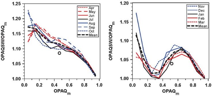
Figure A1. Ratio OPAQSW/OPAQ_m as a function of OPAQ_m for warm season (left) and cold season (right). Open circles are weighted mean of all the data.

However the ECA fits Equation (A1) derived from daily data have substantial uncertainty under low cloud conditions, and we found that the near-zero slope of the T > 0°C fit for OPAQSW < 0.15 in (A1a) appears inconsistent with our climatological datasets, which show a smooth change in the diurnal ranges with opaque cloud over this range. So we refitted the BSRN data with the constraint that ECA = 0 when OPAQSW = 0, giving for the warm season (T > 0^oC) (R² = 0.86)

$\begin{array}{cc}\begin{array}{l}ECA=0.0(\pm 0.09)+0.24(\pm 0.01)OPAQSW\\ +0.47(\pm 0.01)OPAQS{W}^2\end{array}& (\text{A}2\text{a})\end{array}$

For the cold season (T > 0^oC) this fit through the origin is (R² = 0.70)

$\begin{array}{cc}\begin{array}{l}ECA=0.0(\pm 0.11)+0.36(\pm 0.02)OPAQSW\\ +0.15(\pm 0.02)OPAQS{W}^2\end{array}& (\text{A}2\text{b})\end{array}$

The uncertainty under low cloud conditions remains, but we will use Equations (A2) and the mean weighting functions in Figure A1 to derive ECA in Equation (6).