Bayesian Inference of Subglacial Topography Using Mass Conservation

1. Introduction

Bed elevation is required to model glacier dynamics. Measurements are typically performed with spatially localized radar soundings (e.g., Allen et al., 2015) and tend to be precise and dense along a line. However, because modeling often requires a thickness field, reliable methods of interpolation between observations are valuable.

Many widely used digital elevation models (DEMs) of subglacial topography are based upon classical geostatistical techniques such as Kriging (Bamber et al., 2013). Such DEMs tend to induce immediate modeled surface elevation changes from dynamical models that are implausibly larger than observations of surface elevation change (Seroussi et al., 2011; Bindschadler et al., 2013). In an effort to minimize these spurious model transients, contemporary DEMs incorporate physical constraints on interpolated fields. The procedure is conceptually simple and fits neatly into the general framework of geophysical inversion theory: formulate a cost functional that quantifies the misfit between the field of interest and observations, subject to the constraint that the field be compatible with a forward model.

Inverse methods are widely used in glaciology. MacAyeal (1993) presented a method for using the momentum conservation equations to invert for basal shear stress using an observed surface velocity field. The same method has been used over the last 20 years mostly unchanged, though with advances in forward model sophistication and data availability (e.g., Morlighem et al., 2010; Brinkerhoff and Johnson, 2013; Sergienko et al., 2014). Gudmundsson and Raymond (2008) developed a Bayesian approach that used surface elevation, surface elevation trend, and surface velocity, along with strong prior information about the bed elevation to compute the maximum a posteriori estimate of basal shear stress and basal topography. Perego et al. (2014) solved for thickness and basal traction by simultaneously inverting the mass and momentum conservation relations. McNabb et al. (2012) and Morlighem et al. (2014b) used optimal control methods and mass conservation (without an associated momentum conservation model) to infer ice thickness. Brinkerhoff and Johnson (2015) used a similar approach to produce seamless velocity maps of Greenland, filling data gaps in satellite-based velocity estimates with balance velocities. Huss and Farinotti (2012) and Li et al. (2011) used surface geometry with mass conservation to estimate global glacier volume, even in the absence of velocity data. However, Bahr et al. (2014) suggests caution in using mass conservation unconstrained by observations since uncertainty grows exponentially as resolution increases unless short wavelength topography is suppressed.

An important limitation exists in all of the above studies: none rigorously quantify the error bounds of their solutions in the sense that uncertainty estimates are linearized around the optimal solution or estimated empirically by comparison with independent data. Viewed in a Bayesian context, these methods report the maximum a posteriori probability, but not the associated probability distribution. Uncertainty, when reported, is subject to the assumption of a local Gaussian approximation based on an approximately computed Hessian (e.g., Tarantola, 2005, Chapter 3). However, the posterior distribution of an unknown variable often displays richer behavior due to non-linearities in the governing physics and associated covariance structure. If we are to use fields inferred from model inversion to predict glacier evolution, then we must know whether two equally likely instances of these fields can produce qualitatively different conclusions.

Monte Carlo sampling techniques can provide distributions of model parameters. Several examples of the application of Monte Carlo techniques to glaciological problems exist. Petra et al. (2013) developed a Markov Chain Monte Carlo method that generated samples from the posterior basal traction distribution using an efficiently computed approximation to the true Hessian to steer the sampling algorithm. Chandler et al. (2006) randomly perturbed measured surface velocities of Glacier de Tsanfleuron and repeatedly inverted for the associated basal properties. Colgan et al. (2012) used a Monte Carlo technique to characterize the retreat regime of Columbia Glacier over a wide range of unknown model input parameters, using a heuristic filter to eliminate improbable simulations. All of these cases produced samples from probability distributions of unobserved glaciological variables without the assumption of linearization around a fixed point.

In this paper, we use the Metropolis-Hastings (MH) algorithm (Hastings, 1970) to construct probability distributions of ice thickness (and hence bed elevation when surface elevation is know), subject to observations and prior estimates of surface velocity, specific surface mass balance rates (hereafter referred to simply as mass balance), and surface elevation change, as well as sparse pointwise observations of thickness. This situation is common with the recent availability of spatially distributed climate model output and satellite-derived velocity fields. We assume that depth-averaged velocity, thickness, and apparent mass balance (defined here as mass balance minus surface rate of change, Farinotti et al., 2009) are related through mass conservation, and that depth averaged velocities relate to surface velocities in a known albeit unobserved fashion. Each dataset is subject to an assumed covariance structure. This is an analogous problem as that of Brinkerhoff and Johnson (2015), McNabb et al. (2012), and Morlighem et al. (2014b), using mass conservation to interpolate ice thickness estimates while satisfying observational and physical constraints. Contrary to those works, we view the problem from a Bayesian perspective, which allows construction of the full posterior probability density for each model variable. It also serves as an example of how to propogate uncertainty through non-linear glaciological models.

We apply our method to three cases. We begin by considering a synthetically generated glacier, where the simulated velocity, mass balance, and thickness measurements (or prior estimates) are corrupted with noise, and the thickness field is recovered under several assumptions regarding covariance and measurement spacing. We then examine the degree of uncertainty induced by the choice of error structure and physical properties of the glacier. Next, we apply the method to Storglaciären, a ≈ 3 km long alpine glacier where dense measurements of thickness, velocity, and mass balance are available. This provides an interesting test case with which to gauge the uncertainties induced in topographic estimates due to real-world uncertainties. Finally, we apply the method to Jakobshavn Isbræ, the largest outlet glacier on the Greenland Ice Sheet, and assess resulting uncertainty estimates in the context of making a recommendation for flightline spacing during future airborne radar campaigns.

2. Methods

Bayes' theorem states that

$\begin{array}{ll}P(\mathbf{\text{m}}|\widehat{\mathbf{\text{d}}})\propto P(\widehat{\mathbf{\text{d}}}|\mathbf{\text{m}})P(\mathbf{\text{m}}),& \left(1\right)\hfill \end{array}$

where m ∈ ${R}$^m is a vector of unobserved model parameters, and $\widehat{\mathbf{\text{d}}}\in {{R}}^n$ is a vector of observed model outputs (e.g., Tarantola, 2005). P(·) is the probability density function, a quantification of possible parameter values. Bayes' theorem provides a means to formulate the posterior distribution $P(\mathbf{\text{m}}|\widehat{\mathbf{\text{d}}})$ by considering new data, and it is from this distribution we may draw conclusions.

Construction of the posterior requires two components. First, the likelihood $P(\widehat{\mathbf{\text{d}}}|\mathbf{\text{m}})$ characterizes the probability of observing a realization of $\widehat{\mathbf{\text{d}}}$ given m. Evaluation of this term requires a solution to the forward model. Second, the prior model P(m) is the supposed distribution of model parameters prior to consideration of data, including assumptions about the mean, covariance, and bounds.

All inverse problems incorporate prior information in one form or another (smoothness for example), which is necessary because of the ill-posedness of such problems. One particular advantage of Bayesian methods is that these prior assumptions, which are often vacuously defined in other inverse methodologies, are defined precisely here and are subject to scrutiny. Another is that changes in assumptions and the addition of new information are easily incorporated by changing the definitions of likelihood and prior without any structural changes in the inference procedure.

2.1. Observation Process

We define data to be observed quantities that have not been considered when forming the prior distribution. We denote data with a hat. Data may include observations of surface speed ${\widehat{\mathbf{\text{U}}}}_s$, specific surface mass balance $\widehat{\dot{\mathbf{\text{b}}}}$, thickness $\widehat{\mathbf{\text{H}}}$, surface elevation rate of change $\hat{\frac{\Delta \mathbf{\text{S}}}{\Delta \mathbf{\text{t}}}}$, and (map plane) flow direction $\widehat{\mathbf{\text{N}}}$. These components form the data vector

$\begin{array}{ll}\widehat{\mathbf{\text{d}}}=\left[\begin{array}{c}{\widehat{\mathbf{\text{U}}}}_s\\ \widehat{\dot{\mathbf{\text{b}}}}\\ \widehat{\mathbf{\text{H}}}\\ \widehat{\mathbf{\text{N}}}\\ \hat{\frac{\Delta \mathbf{\text{S}}}{\Delta \mathbf{\text{t}}}}\end{array}\right].& \left(2\right)\hfill \end{array}$

Bold indicates a vector: each observation may be available at any number of locations any number of times. We assume that each entry in $\widehat{\mathbf{\text{d}}}$ is a random variable drawn from a distribution about a true mean value. The realization of such a variable is called the observation process. The observation process takes the form

$\begin{array}{ll}\widehat{\mathbf{\text{d}}}~{F}(\mathbf{\text{m}},{\Sigma }_{\mathbf{\text{d}}}),& \left(3\right)\hfill \end{array}$

where m is the vector of model parameters upon which the observation process ${F}$ operates and Σ_d is a parameterization of observational uncertainty induced by the observation process. It includes but is not limited to measurement error. It may be the case that some of the subvectors in $\widehat{\mathbf{\text{d}}}$ are empty, and in this case the distribution of that function is determined by the prior and its relationship to other parameters through the forward model. This is not to say that no observations have been involved; sometimes they have already been used in a different model to formulate a better prior.

2.2. Forward Model

While we assume that the uncertainties Σ_d induced by the observation process are approximately independent (i.e., observational errors at neighboring locations are uncorrelated), the model parameters are not. Thickness H(x), mass balance ḃ(x), and flow direction N(x) specify the depth-averaged speed Ū(x) through the continuity equation

$\begin{array}{ll}{\partial }_{t}H(\mathbf{\text{x}})\approx {\partial }_{t}S(\mathbf{\text{x}})=-\nabla ·\left[\overline{U}(\mathbf{\text{x}})H(\mathbf{\text{x}})\mathbf{\text{N}}(\mathbf{\text{x}})\right]+\dot{b}(\mathbf{\text{x}}),& \left(4\right)\hfill \end{array}$

where ∇· refers to the map plane divergence. We assume that basal melt is negligible. Also, we have used the approximation that thickness rate of change ∂_tH is well approximated by the surface rate of change ∂_tS, which makes the assumption that bed elevations are stationary. This is often a good assumption, though not in regions experiencing rapid subglacial erosion (Motyka et al., 2006).

Equation (4) is valid only at an instant in time. On the contrary, data are observed over finite time intervals. The length of these intervals may vary between observables, and are often not aligned with one another (e.g., velocity may have been observed over the entire winter of 2008, while thickness observations have been taken almost instantaneously during the summer of 2005). Observations may thus be far from the cotemporal and instantaneous values required to make Equation (4) valid. This incongruity in and between the characteristic time scales of the observation and model processes is responsible for an additional source of error that must be accounted for.

One way of constructing a valid mass conservation relationship over the entire observation period is to time integrate the forward model over the range t ∈ [t₀, t₁], where t₀ and t₁ are the starting and ending times over which an estimate of time-averaged quantities are available. Integrating and dividing Equation (4) by the interval Δt = t₁ − t₀ yields

$\begin{array}{ll}\frac{\Delta S}{\Delta t}+\frac{1}{\Delta t}{\displaystyle {\int }_{t_0}^{t_1}}\left(\nabla ·\left[\overline{U}\mathbf{\text{N}}H\right]-\dot{b}\right)dt=0,& \left(5\right)\hfill \end{array}$

the time average over the observation period. Replacing each term with its average yields an equation similar to Equation (4), but with a reinterpretation of observational uncertainty: not only imprecision in direct measurement and processing, but also the departure of the observation from the time average. We write this as

$\begin{array}{ll}{\Sigma }_{\mathbf{\text{d}}}={\Sigma }_{obs}+{\Sigma }_t,& \left(6\right)\hfill \end{array}$

where Σ_obs is uncertainty due to measurement, and Σ_t is the uncertainty due to measurements not being those of direct relevance to the forward model. s Velocity observations are only available at the surface, while the forward model Equation (4) requires depth-averaged quantities. We assume that surface flow directions N are a good approximation of flow direction at depth. However, this is not always true for magnitudes and we introduce a spatially variable multiplicative factor s(x) that serves to transfer between depth-averaged speed and surface speed

$\begin{array}{ll}{U}_s(\mathbf{\text{x}})=s(\mathbf{\text{x}})\overline{U}(\mathbf{\text{x}}).& \left(7\right)\hfill \end{array}$

2.3. Model Simplification

Monte Carlo methods such as the MH algorithm are computationally expensive because the likelihood (and thus the forward model) must be evaluated many times. Fortunately, as long as N(x) is constant with depth, the mass conservation model is purely advective and we can exploit the independence of flow bands (McNabb et al., 2012). If we select two streamlines from the velocity field, the domain contained between them is independent of any other non-overlapping domain. If they are close, we can approximate the parameter variability transverse to flow with the transverse average, and the problem reduces from two dimensions to one. Neglecting curvature effects, the continuity equation becomes

$\begin{array}{ll}{\partial }_r\left[w(r)\overline{U}(r)H(r)\right]=w(r)\left(\dot{b}(r)-\frac{\Delta S(r)}{\Delta t}\right),& \left(8\right)\hfill \end{array}$

where r is the along-flow coordinate, and w(r) is the width of the streamline taken normal to the centerline. Parameters should again be viewed as averages over the temporal footprint of the observations. Note that the flow direction N(x) no longer enters the equation, since it has been subsumed by the width, which has its own observational uncertainty and prior. The model parameter vector is

$\begin{array}{l}\mathbf{\text{m}}=\left[\begin{array}{cc}U(r;H(r),\dot{b}(r),\frac{\Delta S(r)}{\Delta t})& \left(9\right)\hfill \\ H(r)\\ \dot{b}(r)\\ \frac{\Delta S(r)}{\Delta t}\\ s(r)\\ w(r)\end{array}\right].\end{array}$

This one dimensional formulation is efficient because it can be solved by integration:

$\begin{array}{ll}\overline{U}(r)=\frac{1}{w(r)H(r)}{\displaystyle {\int }_0^r}w(r\prime )\left(\dot{b}-\frac{\Delta S(r)}{\Delta t}\right)dr\prime ,& \left(10\right)\hfill \end{array}$

which we evaluate with trapezoidal quadrature (e.g., Atkinson, 1978).

Non-dimensionalization of Equation (10) produces an interesting result: the model depends on only a single non-dimensional parameter,

$\begin{array}{ll}\gamma =\frac{L\tilde{b}}{\tilde{U}\tilde{H}},& \left(11\right)\hfill \end{array}$

where $\tilde{b}$, $\tilde{U}$, and $\tilde{H}$ respectively refer to characteristic mass balance, velocity, and thickness, and L the length of the glacier, and thus it should be understood that results here apply similarly to differently scaled glaciers so long as γ remains constant.

2.4. Priors

The specification of prior distributions on model parameters depends on the variable and the problem being considered. However, a universal requirement is that priors be chosen before considering any of the observations contained in $\widehat{\mathbf{\text{d}}}$.

We assume no prior knowledge of the ice thickness H(r) besides non-negativity and that it possesses some smoothness, and its prior should reflect these properties. This implies some knowledge of the covariance structure of ice thickness. A useful and general representation of H(r) is as a Gaussian process (GP Rasmussen, 2006) with arbitrary mean and large variance, but with a specified covariance structure

$\begin{array}{ll}H(r)~GP(·,{\nu }_H(r,r\prime )),& \left(12\right)\hfill \end{array}$

where ${\nu }_H(r,r\prime )$ is a spatial covariance function. The placeholder · indicates that the mean value should be arbitrary; the prior is sufficiently vague that the value of the mean does not affect the posterior distribution. We modify the Gaussian process so that negative values of H have zero probability. We use either the following Gaussian covariance function

$\begin{array}{ll}{\nu }_i^G(r,r\prime )={\sigma }_i^{2}exp\left(-\frac{{(r-r\prime )}^2}{l_i^2}\right)& \left(13\right)\hfill \end{array}$

or exponential covariance function

$\begin{array}{ll}{\nu }_i^E(r,r\prime )={\sigma }_i^{2}exp\left(-\frac{|r-r\prime |}{l_i}\right),& \left(14\right)\hfill \end{array}$

for the remainder of this paper, where ${\sigma }_i^2$ is the prior variance, r − r′ is the pointwise distance between any two points, and l_i is the correlation length scale. Note that for $|r-r\prime |>3l_i$, values no longer exhibit significant correlation (Rasmussen, 2006).

It is often preferable to specify a mass balance distribution in which the data have already been reanalyzed with a separate climate model or interpolated with some other method since these are more advanced than one we could include. Here we consider the estimated posterior distribution of a climate model to be the prior on mass balance, since observations have already been included. We assume that the mass balance prior is also a Gaussian process

$\begin{array}{ll}\dot{b}(r)~GP({\dot{b}}_{prior}(r),{\nu }_{\dot{b}}^G(r,r\prime )).& \left(15\right)\hfill \end{array}$

We assume that the width function is a Gaussian process with a mean value given by the computed width,

$\begin{array}{ll}w(r)~GP(w_{prior}(r),{\nu }_w^G(r,r\prime )).& \left(16\right)\hfill \end{array}$

The use of a Gaussian process as a prior is the same key assumption as used in Kriging (Williams, 1998), and this technique should be seen as Kriging with additional information introduced to the likelihood function by continuity. Where no observations exist, the algorithm reverts to ordinary Kriging.

Once again, surface velocities and depth-averaged velocities are only equal when sliding accounts for all glacier movement. The other end-member, pure deformation, bounds the value of surface velocity at $U_s(r)=\frac{n+2}{n+1}\overline{U}(r)$, where n = 3 is Glen's flow law exponent (Glen, 1955). This usually holds in polythermal glaciers, where the more complex rheological structure concentrates strain at the glacier base, and makes the depth averaged velocity closer to the surface velocity. We typically have no other a priori information about the sliding proportion s, and thus model it as a uniform distribution with the bounds given by the above argument

$\begin{array}{ll}s(r)~Unif1,\frac{n+2}{n+1}.& \left(17\right)\hfill \end{array}$

2.5. Metropolis-Hastings Algorithm

The posterior distribution has no closed form and must be characterized by sampling. With samples in hand we can evaluate their statistical properties as a proxy for the posterior distribution. Our method of choice for this procedure is the Adaptive Step Metropolis-Hastings algorithm (Hastings, 1970). Pseudocode for the algorithm is given in Algorithm 1.

ALGORITHM 1

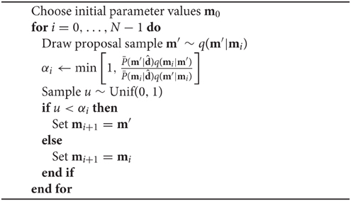
Algorithm 1. Pseudocode describing the Metropolis-Hastings algorithm. Note that q(·|·) is the proposal distribution, and $\overline{P}(·|\mathbf{\text{d}})$ is the product of the likelihood and the prior evaluated at a point. Evaluation of the likelihood requires solution of the forward model.

The MH algorithm operates by traveling through parameter space according to steps drawn from a proposal distribution, in this simple case an independent multivariate normal centered around the current point. If the posterior probability is greater at the proposed point than at the current point, then the proposed step is accepted, and the algorithm continues from the new point. If the likelihood is lower at the proposed point, then a step is taken with probability equal to the ratio of the current and proposed points. In the adaptive step variant of the MH algorithm, the width of the proposal distribution is adjusted such that an optimal proportion of proposals are accepted. The algorithm is ergodic (Hastings, 1970), and after a sufficient number of steps, the samples converge to a set drawn from the posterior distribution. MH sampling is performed using the python package PyMC (Patil et al., 2010).

3. Synthetic Glacier

3.1. Synthetic Glacier Generation

We used the finite element ice sheet model VarGlaS (Brinkerhoff and Johnson, 2013) to generate a synthetic steady state glacier in vertical profile. We neglect effects due to changing width and side drag. The glacier does not slide. The basal topography is given by

$\begin{array}{ll}B(r)=\frac{z_{min}-z_{max}}{L}r-A_{s}sin\frac{2\pi r}{L}\hfill & \left(18\right)\hfill \\ +A_{e}exp-\frac{r+L}{L_e}+G(r),\hfill \end{array}$

where z_min and z_max are minimum and maximum elevations, L is the domain length scale, A_s is the amplitude of a sinusoidal variability, A_e is the amplitude of an exponential term (simulating a steep headwall), L_e the decay rate of the exponential perturbation centered about the bergschrund, and G(r) is a random topographic perturbation given by

$\begin{array}{ll}G(r)~GP(0,{\nu }_T^G(r,r\prime )).& \left(19\right)\hfill \end{array}$

Mass balance is an exponential function of surface elevation.

$\begin{array}{cc}\begin{array}{l}\dot{b}(S(r))={\dot{b}}_{min}+\frac{{\dot{b}}_{max}-{\dot{b}}_{min}}{1-\exp (-c)}\hfill \\ \times \left[1-\exp \left(-c\frac{S(r)-z_{min}}{z_{max}-z_{min}}\right)\right],\end{array}& (20)\end{array}$

where $\dot{b}$_min and $\dot{b}$_max are the mass balance minimum and maximum respectively, and c is a shape parameter. While the scale of the geometry will not be relevant to the results contained herein (q.v. Section 2.3), we performed the computations in dimensional form because it was easier to define reasonable parameter values that way. The parameters used are shown in Table 1, and correspond to a moderate-size maritime mountain glacier. The model was discretized over n_c = 100 equally spaced grid cells and time integrated until reaching a steady state. We assumed that surface elevation was stationary and known exactly.

TABLE 1

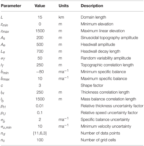
Table 1. Table of relevant constants for the experiment outlined in Sections 3.1 and 3.2.

3.2. Recovery of Synthetic Topography

As a first experiment, we used the MH algorithm to sample m under assumptions of uncertainty and data spacing that might correspond to a typical mountain glacier. First, we simulated observations of surface velocity by corrupting modeled velocity with uncorrelated Gaussian random noise with standard deviation σ_{u, i} = max(p_uU_{m, i}, σ_{u, min}). Thickness measurements were assumed available at Δd = L∕n_d increments. Uncertainties in thickness measurements were assumed to be σ_{H, i} = p_HH_i. The above values were chosen not only to account for hypothetical instrument error, but also to simulate the deviation of measurements from the average required by Equation 5. As discussed above, we assumed that mass balance observations had already been used to update the prior model.

We assumed that the error structure was known, and that the likelihood model was given by

$\begin{array}{ll}\widehat{\mathbf{\text{d}}}~{N}(\mathbf{\text{d}},{\Sigma }_{\mathbf{\text{d}}}),& \left(21\right)\hfill \end{array}$

where ${N}$(d, Σ_d) is a multivariate normal distribution with mean d and covariance Σ_d. The vector d contains model variables evaluated at observation points. We take Σ_d to be a diagonal matrix with entries given by the corresponding observational uncertainties stated above.

We assumed no prior knowledge of the actual thickness values but that the thickness length scale was known, or that l_H = l_T, and that an informative prior model of mass balance with known covariance was available. Covariance amplitude was given by σ_$\dot{b}$ = r_$\dot{b}$max($\dot{b}$) and ${\nu }_{\dot{b}}^G$ was Gaussian with correlation length l_$\dot{b}$.

Using the MH algorithm, we drew $n_i=10^6$ iterations from the posterior distribution of m, discarding the first 10⁵ samples to eliminate transient behavior. We performed this procedure three times, using different (random) initial conditions for each sample. Evidence for the convergence of the samples to a stationary and correct posterior distribution will be demonstrated in Section 3.3.

Figure 1 shows the pointwise posterior distributions of the model parameters in m. The most notable immediate result is that the algorithm produces correct credibility intervals: the 2σ credibility interval does indeed contain the true bed elevation at 95% of grid points, which provides confidence that the posterior distribution produced by the algorithm can recover meaningful information about the bed elevation.

FIGURE 1

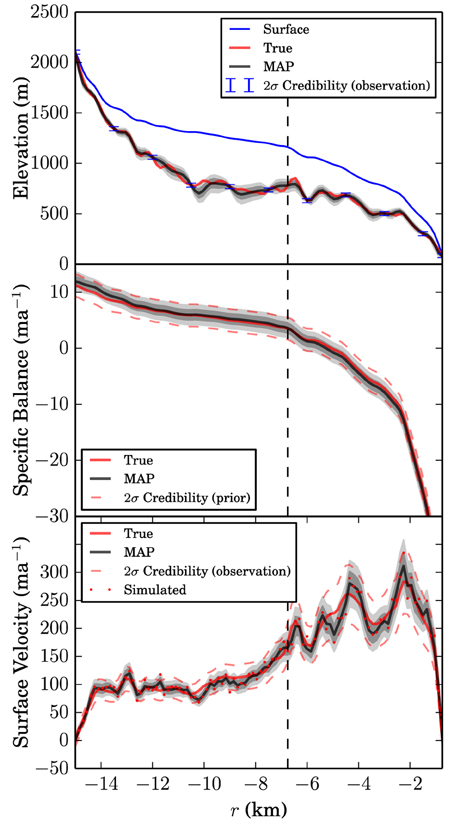
Figure 1. Recovered pointwise probability densities for a synthetic glacier. Dark and light gray shaded regions indicate the σ and 2σ posterior credibility interval respectively, and MAP refers to the solution corresponding to the maximum a posteriori probability. The dashed vertical line is the location at which the histograms in Figure 2 are computed.

Nonetheless, the maximum a posteriori prediction of bed elevations is not the true value. This is not a surprising result, since we assume a single measurement of velocity for a given location with which to constrain the mean of the velocity distribution there (though multiple observations at a point can be included naturally, see Section 4.1). The mean velocity is thus free to assume values in the space around the observation, but the most probable value of the velocity mean given one observation per grid point and in the absence of feedbacks from additional constraints on the velocity is the data point itself.

An interesting feature of the posterior distributions of both mass balance and surface velocity is that the posterior distribution is more specific than the prior. This implies that not only are these fields contributing information to the estimation of thickness, but data and smoothness constraints on the thickness also feed back.

3.3. Convergence

There are several mechanisms for assessing whether a distribution has become stationary, some heuristic and some quantitative. For a good approximation to the posterior distribution to be achieved, (a) the sampler must traverse the support of the sampled function many times, (b) the sampler must visit the entire support, and (c) the region traversed by the sampler should be insensitive to initial conditions.

Examining traces (i.e., the history of parameter values at each sampler iteration) gives a heuristic means to assess convergence. Figure 2A shows the traces of the model vector m at the location indicated by the vertical dashed line in Figure 1. These plots are similar at any location. The “fuzzy” pattern is an indication that the samples are well-mixed, which is to say that both criteria (a and c) are satisfied. While it is difficult to state definitively that there is not a distant probability maximum that is not being captured, this is unlikely due to physical intuition and the wide dispersion of initial conditions between samplers.

FIGURE 2

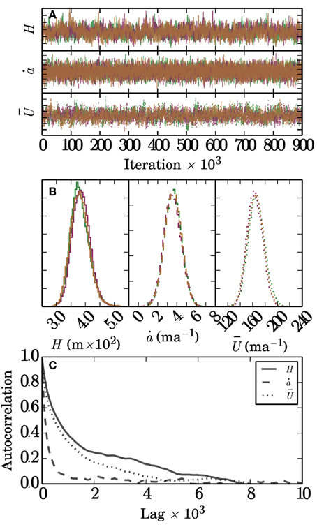
Figure 2. Convergence metrics for the grid point denoted by a vertical dashed line in Figure 1. (A) The trace for each sampler and for each variable. The traces indicate full exploration of the parameter space. (B) histograms of each variable for each sampler. (C) The auto-correlation for thickness H, mass balance $\dot{b}$, and speed U_s. For example, samples for thickness H become uncorrelated after approximately 8000 iterations.

Figure 2B shows the posterior probability for several model variables. The densities associated with each sampler exhibit a high degree of similarity, which is further evidence that the samples produced by the MH algorithm have converged to the stationary posterior distribution.

The Gelman-Rubin statistic (Gelman and Rubin, 1992) provides a quantitative convergence statistic. This statistic compares the ratio between the interchain variance

$\begin{array}{ll}B=\frac{n}{m-1}{\displaystyle \sum _{j=1}^m}{({\overline{\mathbf{\text{m}}}}_j-\overline{\overline{\mathbf{\text{m}}}})}^2,& \left(22\right)\hfill \end{array}$

and the within-chain variance

$\begin{array}{ll}W=\frac{1}{m}{\displaystyle \sum _{j=1}^m}\left[\frac{1}{n-1}{\displaystyle \sum _{i=1}^n}{({\mathbf{\text{m}}}_{ij}-{\overline{\mathbf{\text{m}}}}_j)}^2\right],& \left(23\right)\hfill \end{array}$

where we have m chains each of length n, ${\overline{\mathbf{\text{m}}}}_j$ is the mean of chain j, and $\overline{\overline{\mathbf{\text{m}}}}$ is the mean of all chains. The marginal posterior estimate of the variance of m can be estimated by

$\begin{array}{ll}\widehat{Var}(\mathbf{\text{m}}|\widehat{\mathbf{\text{d}}})=\frac{n-1}{n}W+\frac{1}{n}B.& \left(24\right)\hfill \end{array}$

This quantity always overestimates the true value of the marginal variance. Simultaneously, W underestimates the within-chain variance for an underconverged chain. Thus, in the limit as n → ∞, the ratio of these two quantities

$\begin{array}{ll}R=\frac{\widehat{Var}(\mathbf{\text{m}}|\widehat{\mathbf{\text{d}}})}{W}& \left(25\right)\hfill \end{array}$

converges to one. Thus, for a fully converged distribution (i.e., one that exhibits behavior similar to the limiting case), R ≈ 1. In practice, R < 1.1 is acceptable (Gelman and Rubin, 1992). We find that for each component in m, R ≪ 1.1, providing evidence that the samples are drawn from the stationary distribution.

Figure 2C addresses a final numerical consideration. The MH algorithm produces samples that are autocorrelated, which can persist when parameters covary (as is usually the case with spatial processes). While this auto-correlation is not fatal to the algorithm's performance, it provides an important reminder to run each chain long enough to obtain unbiased sample statistics (Christensen et al., 2011; Link and Eaton, 2012). The Gelman-Rubin statistic suggests that the MH algorithm has been run long enough to overcome the difficulties due to autocorrelation.

3.4. Uncertainty Propagation

The relative uncertainty with which the ice thickness can be recovered using mass conservation methods is a function of the relative uncertainties and covariance structures of surface velocity measurements, mass balance measurements (or assimilated model output), ice thickness measurements, and ice thickness measurement density. It is reasonable to suspect that an improvement in any of these factors would lead to a commensurate improvement in posterior predictive capabilities with respect to thickness. Nonetheless, it is not clear which of these factors contributes the lion's share of posterior variance. This information is key in forming plans of additional data acquisition; we would like to know which data improvements (and at what densities) will most improve thickness estimates.

Here we examine the influence that surface velocity uncertainty, mass balance uncertainty, and measurement density have on the relative thickness uncertainty (quantified here as $\langle {\sigma }_H\rangle ∕\tilde{H}$). We neglect to consider sensitivity to uncertainty in thickness measurements. However, these uncertainties may well be important in many cases, particularly if the assumption of on-nadir bed returns is flawed or if these exhibit systematic errors. The assumption of a normally distributed error structure may also be inappropriate. Nonetheless, we proceed without a detailed quantification of these effects because (a) the quantification of radar uncertainty is not the focus of this paper and (b) we do not know the most appropriate way to proceed. However, it would be straightforward to include such a detailed uncertainty estimate within the framework presented here.

In order to assess the functional relationship between these uncertainties, we performed simulations over an array of 10 equally spaced relative velocity uncertainties between 0 and 20% of the true maximum surface velocity, 10 relative mass balance uncertainties between 0 and 50% of the true maximum mass balance, and the number of data points n_d ∈ {11, 6, 3}. Note that the last of these data spacings n_d = 3 corresponds to a thickness measurement at the midpoint of the glacier, along with the constraints of zero thickness at the glacier head and terminus. This corresponds to 300 simulations, each of which was run to convergence.

Figure 3A shows the mean standard deviation in thickness (normalized by max thickness) as a function of the mean velocity standard deviation (normalized by maximum velocity). Solid lines correspond to the case where the mass balance is known very precisely (σ_$\dot{b}$ = 0), while the dashed lines represent an intermediate uncertainty in mass balance $(\langle {\sigma }_{\dot{b}}\rangle )/\tilde{b}=0.25$. Thickness and velocity uncertainties exhibit a linear relationship. The proportionality depends weakly on data density because of the lack of a smoothness constraint directly imposed on velocity; it is strictly a function of thickness and mass balance and only indirectly sees the locations at which thickness is known. Where mass balance is known precisely, the n_d = 3 and n_d = 6 solutions are similar. This is because the variance in velocities admissible with respect to forward model constraints when only a single measurement of thickness exists is less than the variance in velocity due to measurement uncertainty. When mass balance has large uncertainty, the forward model imposes a weaker constraint and the distribution of velocities becomes progressively wider as observational uncertainty increases.

FIGURE 3

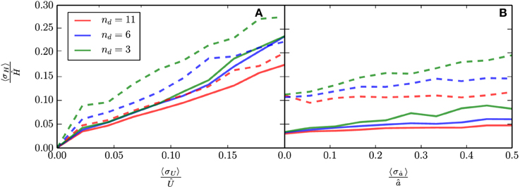
Figure 3. Relationship between average thickness uncertainty and velocity uncertainty (A) and mass balance uncertainty (B). Solid lines reflect the case where the other variable is being held constant at a low level of uncertainty (e.g., mass balance held fixed while velocity is varied), while dashed lines represent the case where the other variable is held constant at a high uncertainty. These curves are computed for three different data densities.

Thickness precision as a function of mass balance uncertainty (Figure 3B) is also linear. However, this relationship depends more on data density due to the long correlation length imposed upon mass balance. While it can assume many values between thickness measurements, the local constraint imposed by mass conservation at thickness measurement locations forces it to a unique value there. If the measurement spacing is shorter than the mass balance correlation length, it cannot vary much between these two pinned points, regardless of its variance. This constraint becomes less active as measurement spacing increases, allowing the uncertainty in mass balance to more strongly influence uncertainty in the thickness.

4. Storglaciären

4.1. Characterization and Data

Storglaciären is a ≈ 3 km long polythermal glacier in northwestern Sweden. It possesses the longest spatially distributed surface mass balance record of any glacier (Holmlund et al., 2005). The relative simplicity of its geometry along with the density of mass balance data make it a useful test case. Also, the basal topography of Storglaciären is well known and thus this experiment provides a means to assess whether the algorithm correctly produces error bounds on a “known” bed.

Thickness and surface observations were adapted from Herzfeld et al. (1993). Surface velocities were derived from stake measurements (Hooke et al., 1989; Jansson, 1997; Kuriger, 2002). These observations are discrete rather than fields. However, this distinction from the previous synthetic example provides no particular difficulty from a technical standpoint.

We estimated the flowline width by using a first order glacier flow model (Brinkerhoff and Johnson, 2013) in the full map-plane domain to invert point measurements of surface speed for basal traction. We used the resulting velocity field to compute a flowband with centerline coordinates that passed approximately through the velocity observation points. We did not use this modeled velocity field as an observation. Instead, to reduce circularity, we used the original measurements.

A prior distribution on mass balance was generated from the measured annual net balance for Storglaciären between years 2000 and 2013 (Jansson, 1999). The availability of multiple years of data allowed the computation of both the sample mean and the estimated covariance of the mean as a function of surface elevation. A spatial covariance function ${\nu }_{\dot{b}}^G(S(r),S(r^{\prime }))$ was computed by fitting the sample mean covariance matrix with a Gaussian covariance function, similar to Equation (14). This covariance function was parameterized as a function of surface elevation.

Thickness measurement uncertainty was assumed to be σ_H = 10 m, and the thickness field was assigned a vague prior as in the synthetic case. We assumed a correlation length of l_H = 250 m, a velocity standard deviation of σ_u = 5 ma⁻¹, and a width uncertainty of σ_w = 0.1. The Storglaciären flowline was discretized with a horizontal resolution of approximately 35 m. Despite profile data being given as continuous, we artificially sampled the thickness every 350 m.

4.2. Recovery of Known Topography

We ran the Metropolis-Hastings algorithm three times for 10⁶ iterations each, discarding the first 10⁵ samples. Each instance was given different initial values drawn from the prior distribution. We assessed the convergence of the samples using the same methods as discussed in Section 3.3. This analysis produced similar results to those of the synthetic case (not shown).

Figure 4 shows the computed posterior distributions and priors. The credibility intervals provide a correct if conservative estimate of the true value. However, it is not clear that in the presence of a large number of data points and a smooth bed (as for Storglaciären), that much is to be gained by using a mass conservation based interpolant. Rather, ordinary Kriging or some variant thereof would be equally useful in establishing a bed elevation model for dynamic modeling. This is less an indictment of mass conservation methods and more a reflection of the fact that Storgläciaren's simple topography, smooth bed, and high data density make for an ideal case for Kriging. Despite the fact that Storglaciären has a well constrained mass balance, we have already shown that the mass conservation method is insensitive to this quantity in cases where thickness measurements are closely spaced, and this dataset cannot be fully utilized. Simultaneously, surface velocities are discrete, and mass conservation cannot contribute much between observation locations. Nonetheless, the mass conservation technique produces a distribution that would be useful in forcing ensemble runs with dynamic models. Furthermore, it produces an estimate of unobserved surface velocities and a corresponding uncertainty estimate.

FIGURE 4

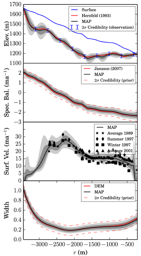
Figure 4. Recovered pointwise probability densities for Storglaciären. Dark and light gray shaded regions indicate the σ and 2σ posterior credibility interval, respectively.

5. Jakobshavn Isbræ

5.1. Characterization and Data

Jakobshavn Isbræ is the largest basin (as ranked by discharge) on the Greenland ice sheet and is the fastest glacier on earth (Rignot and Kanagaratnam, 2006). It drains 7% of the Greenland ice sheet by area. Due to these factors it is comparatively well studied. However, because of the large areal extent the absolute data density compared to Storglaciären (for example) is low.

Absolute mass balance rates over the ice sheet are small compared to a mountain glacier, with a maximum accumulation of around half a meter per year, an order of magnitude lower than a typical mountain glacier. Relative measurement errors are large given identical methods, and the distances over which measurements must be extrapolated are longer. Surface velocities range over four orders of magnitude and relative errors are high in the low velocity interior of the ice sheet and low in the fast flowing outlet regions. Soundings of ice thickness are made by airborne radar in the form of discrete radar flightlines, mostly running normal to the dominant ice flow direction. These can have high observational uncertainty in topographically complex regions (Gogineni et al., 2014).

We consider the time domain t ∈ [2003, 2014] since it overlaps observations of ice thickness (2011–2014, Allen et al., 2015), surface velocity (2008, Rignot and Mouginot, 2012), surface rate of change (2003–2007, Csatho et al., 2014), and mass balance (1958–2007, Ettema et al., 2009). We will describe each of these data sets and our estimate of their uncertainties in this application below.

We extracted a flowband from Jakobshavn Isbræ flowline by generating two streamlines from the InSAR derived velocity dataset of Rignot and Mouginot (2012) (see Figure 5). The streamlines were spaced approximately 100 m apart at a location approximately 50 km upstream of the 2008 terminus location. The flowline used in this section is the centerline between these two flowlines, and all data are assumed to be width-averaged values contained therein. The width itself is the distance between the two flowlines along a line segment normal to the centerline. We assume a uniform 5% standard deviation in flowline width (i.e., σ_w = 0.05).

FIGURE 5

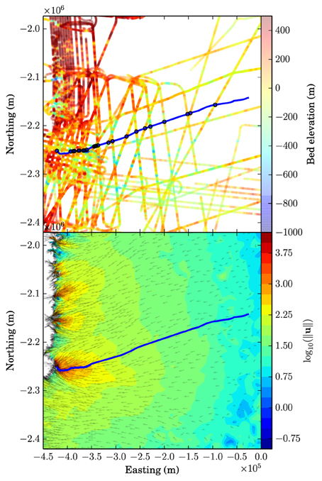
Figure 5. Centerline of the flowband considered for Jakobshavn Isbræ(Blue). Also shown are log-scaled velocity vectors from Rignot and Mouginot (2012), and bedrock elevations along Operation IceBridge flightlines derived from MCoRDS ice penetrating radar (Allen et al., 2015).

Velocity magnitudes were also derived from Rignot and Mouginot (2012). Reported velocity uncertainties are approximately 10 ma⁻¹ due to instrument and processing error. The velocity field spans the single winter of 2008, and as such can account for neither interannual nor intraannual variability, yet there is a considerable amount of spatial and temporal variability in the basin's velocity field. For example, Joughin et al. (2012) showed that in the nearest 40 km to the Jakobshavn Isbræ terminus, velocities could vary by as much as 40% over the course of a year. Additionally, they show a long term trend in velocity over the period between 2004 and 2011. In each case, the degree of temporal variability was spatially heterogeneous, but roughly corresponded to the magnitude of the velocity. Observerations did not always demonstrate a consistent seasonal signal and we cannot assume that the winter observation represents an annual velocity minimum.

A simple uncertainty estimate that can account for the factors given above assumes that observations have an uncertainty of σ_U = max(Û_sp_U, σ_{U, min}). We take σ_{U, min} = 10 ma⁻¹ as a reflection of the instrument uncertainty, a lower bound on the true uncertainty in annual average. We assume p_U = 0.1, which would correspond to a 2σ bound capturing the 40% intraannual variability seen at some locations. While we believe that these uncertainties are roughly representative, we also acknowledge that there are more precise ways to parameterize this uncertainty, for example computing sample covariance between different velocity datasets and using a non-normal uncertainty distribution to reflect the fact that using solely a winter velocity skews the estimate of the mean velocity downwards.

Mass balance was drawn from the regional climate model RACMO2/GR (Ettema et al., 2009), averaged over a period between 1958 and 2007, which is the longest temporal footprint of the data sets considered here. It lacks a covariance estimate, so we assume an uncertainty of σ_$\dot{b}$ = 0.2 ma⁻¹ that reflects the fundamental uncertainty of the model output due to the long distances between controlling data points, systematic uncertainty in the reanalysis process, and processes such as basal melt and surface refreezing that might not be captured. It also accounts for uncertainty induced as a result of using this 49 year average as a proxy for the 11 year average we consider here. We assume a correlation length of l_$\dot{b}$ = 50 km.

The Greenland ice sheet is not in steady state (Motyka et al., 2010; Joughin et al., 2012; Csatho et al., 2014). To account for this, we specify a thickness change field from Csatho et al. (2014). This field is derived from repeat surface altimetry measurements taken between 2003 and 2009. Surface laser altimetry is precise and we thus assume measurement uncertainty in thickness change to be negligible compared to the uncertainty in mass balance estimates. Nonetheless, because the period of record is not contemporaneous with the specified averaging period, we assume that uncertainty in the average thickness rate of change contributes an additional σ_Ht = 0.1 ma⁻¹ to uncertainty in apparent mass balance.

We utilize ice thickness data obtained by aerial radar using the Multichannel Coherent Radar Depth Sounder (MCoRDS) (Allen et al., 2015), collected as part of Operation IceBridge, wherever it intersects the flowline (see Figure 5). Note that we did not include pre-IceBridge observations with the same instrument, instead saving these for validation purposes. However, if we intended to produce a bed elevation field for further modeling use, we would include these observations when computing the posterior distribution. We assume a nominal standard deviation along the flightlines of 12.5 m, as specified in the data documentation. Furthermore, we keep only measurements that are rated as being of “high quality.” This latter filter has the effect of eliminating most radar returns in the deep trough near Jakobshavn Isbræ's terminus, where off-nadir reflections make interpretation of radargrams uncertain. We neglect the small uncertainty resulting from thickness changes over the averaging period.

Variograms computed for IceBridge and pre-IceBridge data have placed the average range (the distance at which samples become uncorrelated) for Greenland between 58 km (Morlighem et al., 2013) and 80 km (Bamber et al., 2001) (erroneously referred to as the sill in both). Both of the above studies fit an exponential covariance model (Rasmussen, 2006). We computed spatially explicit variograms over a moving 120 km footprint for all of Greenland. In the Jakobshavn Isbræ basin, we echo previous work in finding that the exponential model provides the best fit, with an average correlation length of approximately 10 km (the correlation length scale is 1/3 the range). In contrast, the average value over the ice sheet is approximately 25 km. These values are not precise because the assumption of independent samples in the computation of an empirical variogram is violated: nearby samples tend to be oriented parallel or perpendicular to flow. Therefore, we use these values as a guide for specifying the test length scales l_H ∈ [10, 25, 40] km.

5.2. Recovery of Basal Topography for Three Correlation Lengths

We again ran the Metropolis-Hastings algorithm three times for 10⁶ iterations each, discarding the first 10⁵ samples, and each instance was given different initial values drawn from the prior distribution. We assessed the convergence of the samples using the same methods as discussed in Section 3.3, and consideration of traces, histograms drawn from different samplers, and the Gelman-Rubin statistic all indicated sampler convergence.

Figure 6 shows the pointwise posterior distributions produced by the MH algorithm for the flowline described above using l_H = 10 km. It is readily apparent that the bed elevation models of both Bamber et al. (2013) and Morlighem et al. (2014a) are admissible under the posterior distribution produced here, and neither is more probable than the other. The pre-IceBridge observations that were held back are also distributed according to the bounds produced by the posterior distribution, providing evidence for the predictive capabilities of the Bayesian approach.

FIGURE 6

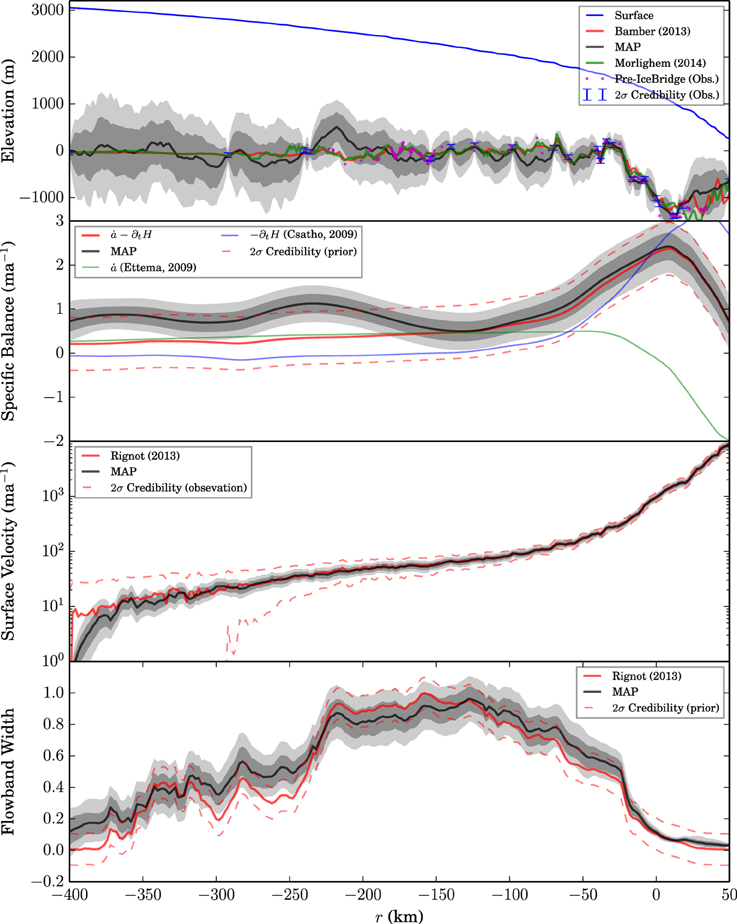
Figure 6. Recovered pointwise probability densities for a flowband over Jakobshavn Isbræ. Dark and light gray shaded regions indicate the σ and 2σ posterior credibility interval, respectively. Also included are the digital elevation models of Bamber et al. (2013) and Morlighem et al. (2014a), as well as pre-Icebridge radar observations that were not included in the solution procedure (Allen et al., 2015).

The algorithm makes significant adjustments to the mass balance and width functions in order to accomodate velocity observations, particularly in the ice sheet interior. The requirement that the algorithm finds a posterior mass balance distribution that is improbable with respect to the prior distribution implies that at least one of the data sets considered herein may have a mean that is far from the true value. One hypothesis is that the surface mass balance model is underestimating aeolian snow redistribution.

Figure 7 shows the influence of correlation length on uncertainty estimates. Also included are the results of the method with the mass conservation relationship ignored, which is equivalent to ordinary Kriging. In regions of slow flow and relatively high uncertainty in velocity and mass balance rates, the uncertainty in derived thicknesses away from observations is large, and this is insensitive to correlation length. This is the case where mass continuity errors produce a similar amount of uncertainty to kriging because it contains little useful information. Conversely, in regions of high data density, the covariance structure on thickness dominates. The smoothness constraint tends to dominate mass conservation, and considering the latter provides no advantage over Kriging in terms of precision. In the intermediate case, where thickness observations are sparse, but relative errors in the other constituents of the mass conservation model are low, the mass conserving interpolation scheme shines, producing uncertainties of less than half the Kriged case. The influence of correlation length on uncertainty estimates is also apparent: longer correlation lengths (i.e., smoother topography) produce lower uncertainties for a given data density.

FIGURE 7

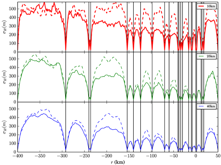
Figure 7. Posterior standard deviations of Jakobshavn Isbræ flowband under different assumptions about the correlation length. Flightline locations are denoted by a vertical black line.

6. Discussion

6.1. Application to the Map-Plane

The method presented herein was limited to the flowline case, and we argue that this context is useful for assessing the uncertainty that we expect from using mass conservation methods. However, many modeling applications require fields over the map plane. Because Monte Carlo methods require the solution of a forward model many times, the transition from solving the balance velocity equation on a flowline, which requires only quadrature, to the map plane, which requires the solution of a linear system of equations (not to mention an inherently greater number of degrees of freedom) is inherently expensive. However, this is not to say that the problem is intractable; because the Metropolis-Hastings algorithm is subject to the Ergodic Theorem, it is efficiently parallelizable in the sense that rather than running a single instance of the algorithm for many iterations, we can run many (independent) instances of the algorithm, and concatenate the resulting samples (Murray, 2010). Aside from this numerical concern, the framework for utilizing the method in the map plane is given in Section 2.2 but without the simplifying assumptions of Section 2.3.

6.2. Selection of Covariance Models

The application of a geostatistical interpolation technique requires the selection of a model for the spatial covariance of the field in question, in this case ice thickness. In Bayesian methods this involves the a priori assumption of a correlation function with the specific form thereof derived from an empirical variogram or some other source (Herzfeld et al., 1993; Bamber et al., 2001). Algorithms that cast the interpolation problem as one of PDE-constrained optimization impose an equivalent smoothness requirement through regularization (Morlighem et al., 2011). In either case, this choice introduces an influence on the pointwise posterior distribution of ice thickness of similar order to that of the mass conservation relationship.

These two processes (covariance function definition and regularization) are equivalent: regularizing on the square of the gradient is the same as using a Gaussian covariance function. The regularization parameter thus has physical relevance in that it is proportional to correlation length, and care must be taken in the selection of a smoothness parameter. It is not appropriate to regularize away the non-uniqueness of the problem with L-curve analysis because this selects the smoothest solution for which the data retains a good fit. However, this level of smoothness may not be physically mandated, and would tend to reduce the feasible range of solutions. Furthermore, the selection of a particular norm on the thickness gradient to minimize has the effect of choosing a covariance function. Experimental variograms suggest that the appropriate model for Greenland is usually exponential, yet the 2-norm regularization commonly used in basal topography inversions implies a Gaussian covariance. This may be desirable if a large scale volume estimate is the goal (Bahr et al., 2014), but for local scale topographic estimation, it produces the wrong result. Instead, the degree of regularization or the covariance structure should be informed by independent analysis of bed covariance, and this must be incorporated into uncertainty estimates.

Nonetheless, deducing the appropriate covariance model and associated parameters is a difficult task, due to the sparsity of bedrock elevation measurements. This is compounded by the fact that glacier flow tends to produce landscapes with anisotropic topographic variability. This variability is spatially heterogeneous, and ice sheet interiors may have different geomorphic properties than the ice sheet margin or heavily glaciated mountain regions. The problem should be addressed by detailed radar soundings of ice thicknesses over regions deemed geomorphically representative of large scale conditions, as well as through analysis of recently deglaciated terrain. For ice sheets, this includes understanding the topographic variability in the heretofore less observed interior regions.

6.3. Flightline Spacing

The selection of bed elevation measurement spacing is of great importance for future data acquisition campaigns, both in mountain and ice sheet environments. Considering Figure 7, and to a lesser extent Figure 3, there is an intermediate spacing regime over which mass conservation techniques can improve thickness uncertainty estimates. For long measurement spacing (i.e., greater than 20 ice thicknesses), mass conservation techniques may or may not outperform Kriging, depending on observational uncertainty. In either case, knowledge of the covariance structure does not improve uncertainty estimates, and errors may be large. For densely spaced flightlines, mass conservation does not offer an advantage over Kriging, because the smoothness imposed by the covariance model overrides any additional information due to continuity. Between these, mass conservation offers improvements in precision. We estimate this efficiency window to be one to two times the correlation length.

For Jakobshavn Isbræ, if we take the available ice-sheet wide empirical variograms computed from collected flightlines as guidance, then an isotropically oriented measurement spacing of approximately 10–20 km is appropriate. A more detailed look at existing measurements, particularly with an eye for discerning anisotropy in topographic covariance could improve estimates of uncertainty. This analysis could be improved further by collection of high density radar measurements over patches in order to better understand the short range topographic correlation structure that governs smoothness. For accurate assessment of the covariance structure, these patches would need to be at least 3 times the correlation length to a side. Regardless of topographic correlation structure, the admissible measurement spacing for a desired accuracy increases given more precise mass balance measurements (above a certain measurement spacing) and more precise velocities (to a point).

7. Conclusions

We have developed a Bayesian statistical model for inferring the posterior probability distribution of ice thickess given sparse observations thereof, coupled with observations of mass balance and surface velocity. Model variables are represented with Gaussian processes, which allow the specification of a covariance structure and prior information. These three parameters are linked through mass continuity. Our work advances upon previous methods in a few primary ways.

The continuity equation must be reformulated from acting instantaneously to over a finite time period. This point is subtle, because the resulting equation is similar to the original. However, the interpretation of the variables involved as time averages induces an additional step in the observation process, and we hence include an additional source of uncertainty (on top of measurement uncertainty) representing the deviation of observed quantities from their averages over the chosen averaging period of the continuity equation. Further constraining the form and magnitude of this uncertainty will be an important advance toward improving continuity-based interpolation schemes.

The Bayesian perspective allows the critical assumptions made in this model process to be elucidated. When assumptions of normality are used, they must be used explicitly. However, the method is general and assumptions of normality are not required. For example, this generality allows us to use a uniform distribution to model the relationship between surface and depth-averaged velocity.

Using Gaussian processes to represent fields such as thickness and mass balance allows for a straightforward and general way to impose smoothness constraints. We reiterate that there is a strong relationship between spatial covariance structure and regularization, and an accurate assessment of this value is critical in accurate modeling of basal topography as well as in determining the precision of those estimates.

For uncertainty estimates typical of velocities, mass balance, thickness, and data density in a mountain glacier, the algorithm reconstructed the basal topography, the distribution of which showed a relative uncertainty (as quantified by the normalized standard deviation) of around 10% at locations far from thickness measurement locations. Thickness uncertainty varies almost linearly with velocity uncertainty, due to the lack of an imposed covariance structure on velocity. On the contrary, the propogation of mass balance uncertainties is also influenced by the length scale of permissible variability in thickness and mass balance itself, as well as by data densities.

Application of the method to Storglaciären, a 3.1 km mountain glacier in the mountains of Sweden was successful, though the resulting uncertainties were relatively large. This is a result of the sparse nature of velocity measurements there, as well as the relatively large uncertainties in long-term average mass balance due to the high degree of interannual variability evident in the mass balance record.

At Jakobshavn Isbræ, the algorithm produced bed estimates with uncertainties varying greatly as a result of data density and relative uncertainty in different regions of the ice sheet. Consideration of mass conservation can improve thickness estimates in regions of low relative velocity and mass balance error, but tends to produce large uncertainties in regions of slow flow and small mass balance. We found that estimates of thickness uncertainty also depended strongly on correlation structure, which is equivalent to regularization in the PDE-constrained optimization context. Obtaining a better estimate of covariance structure would facilitate further application of mass conserving algorithms to ice sheets.

Based on our analysis, we suggest a flightline spacing of one to two times the topographic correlation length in order to best leverage mass conservation based interpolation techniques. For the Jakobshavn Isbræ region, we estimate this spacing to be between 10 and 20 km, but more work is necessary to determine the ideal value for the remainder of the ice sheet.

Author Contributions

DB developed the method and wrote the paper. AA and MT provided critical insight into validity of model assumptions and methodology.

Conflict of Interest Statement

The authors declare that the research was conducted in the absence of any commercial or financial relationships that could be construed as a potential conflict of interest.

Acknowledgments

DB was supported by NSF Graduate Research Fellowship grant number DGE1242789. AA was supported by NASA grants NNX13AM16G and NNX13AK27G. MT was supported by NSF grant PLR 1107491. Thanks to Jesse Johnson, Ron Barry, Regine Hock, Christina Carr, and Ed Bueler for discussions and review that led to great improvements to the manuscipt.

References

Allen, C., Leuschen, C., Gogineni, P., Rodriguez-Morales, F., and Paden, J. (2015). IceBridge MCoRDS L2 Ice Thickness for Greenland. National Snow and Ice Data Center Distributed Active Archive Center.

Atkinson, K. E. (1978). An Introduction to Numerical Analysis. New York, NY: Wiley.

Google Scholar

Bahr, D. B., Pfeffer, W. T., and Kaser, G. (2014). Glacier volume estimation as an ill-posed inversion. J. Glaciol. 60, 922–934. doi: 10.3189/2014JoG14J062

CrossRef Full Text | Google Scholar

Bamber, J. L., Griggs, J. A., Hurkmans, R. T. W. L., Dowdeswell, J. A., Gogineni, S. P., Howat, I., et al. (2013). A new bed elevation dataset for Greenland. Cryosphere 7, 499–510. doi: 10.5194/tc-7-499-2013

CrossRef Full Text | Google Scholar

Bamber, J. L., Layberry, R. L., and Gogineni, S. P. (2001). A new ice thickness and bed data set for the Greenland Ice Sheet 1. measurement, data reduction, and errors. J. Geophys. Res. 106, 33773–33780. doi: 10.1029/2001JD900054

CrossRef Full Text | Google Scholar

Bindschadler, R. A., Nowicki, S., Abe-Ouchi, A., Aschwanden, A., Choi, H., Fastook, J., et al. (2013). Ice-sheet model sensitivities to environmental forcing and their use in projecting future sea level (the SeaRISE project). J. Glaciol. 59, 195–224. doi: 10.3189/2013JoG12J125

CrossRef Full Text | Google Scholar

Brinkerhoff, D., and Johnson, J. (2015). A stabilized finite element method for calculating balance velocities in ice sheets. Geosci. Model Dev. 8, 1275–1283. doi: 10.5194/gmd-8-1275-2015

CrossRef Full Text | Google Scholar

Brinkerhoff, D. J., and Johnson, J. V. (2013). Data assimilation and prognostic whole ice sheet modelling with the variationally derived, higher order, open source, and fully parallel ice sheet model VarGlaS. Cryosphere 7, 1161–1184. doi: 10.5194/tc-7-1161-2013

CrossRef Full Text | Google Scholar

Chandler, D. M., Hubbard, A. L., Hubbard, B. P., and Nienow, P. W. (2006). A Monte Carlo error analysis for basal sliding velocity calculations. J. Geophys. Res. 111:F04005. doi: 10.1029/2006JF000476

CrossRef Full Text | Google Scholar

Christensen, R., Johnson, W., Branscum, A., and Hanson, T. E. (2011). Bayesian Ideas and Data Analysis: An Introduction for Scientists and Statisticians. Cambridge, MA: CRC Press.

Google Scholar

Colgan, W., Pfeffer, W. T., Rajaram, H., Abdalati, W., and Balog, J. (2012). Monte Carlo ice flow modeling projects a new stable configuration for Columbia Glacier, Alaska, c. 2020. Cryosphere 6, 1395–1409. doi: 10.5194/tc-6-1395-2012

CrossRef Full Text | Google Scholar

Csatho, B. M., Schenk, A. F., van der Veen, C. J., Babonis, G., Duncan, K., Rezvanbehbahani, S., et al. (2014). Laser altimetry reveals complex pattern of Greenland Ice Sheet dynamics. Proc. Natl. Acad. Sci. U.S.A. 111, 18478–18483. doi: 10.1073/pnas.1411680112

PubMed Abstract | CrossRef Full Text | Google Scholar

Ettema, J., van den Broeke, M. R., van Meijgaard, E., van de Berg, W. J., Bamber, J. L., Box, J. E., et al. (2009). Higher surface mass balance of the Greenland Ice Sheet revealed by high-resolution climate modeling. Geophys. Res. Lett. 36:L12501. doi: 10.1029/2009GL038110

CrossRef Full Text | Google Scholar

Farinotti, D., Huss, M., Bauder, A., Funk, M., and Truffer, M. (2009). A method to estimate the ice volume and ice-thickness distribution of alpine glaciers. J. Glaciol. 55, 422–430. doi: 10.3189/002214309788816759

CrossRef Full Text | Google Scholar

Gelman, A., and Rubin, D. (1992). A Single Series from the Gibbs Sampler Provides a False Sense of Security. Oxford, UK: Oxford University Press.

Google Scholar

Glen, J. W. (1955). The creep of polycrystalline ice. Proc. R. Soc. A 228, 519–538. doi: 10.1098/rspa.1955.0066

CrossRef Full Text | Google Scholar

Gogineni, S., Yan, J.-B., Paden, J., Leuschen, C., Li, J., Rodriguez-Morales, F., et al. (2014). Bed topography of Jakobshavn Isbrae, Greenland, and Byrd Glacier, Antarctica. J. Glaciol. 60, 813–833. doi: 10.3189/2014JoG14J129

CrossRef Full Text | Google Scholar

Gudmundsson, G. H., and Raymond, M. (2008). On the limit to resolution and information on basal properties obtainable from surface data on ice streams. Cryosphere 2, 167–178. doi: 10.5194/tc-2-167-2008

CrossRef Full Text | Google Scholar

Hastings, W. K. (1970). Monte Carlo sampling methods using Markov Chains and their applications. Biometrika 57, 97–109. doi: 10.1093/biomet/57.1.97

CrossRef Full Text | Google Scholar

Herzfeld, U. C., Eriksson, M. G., and Holmlund, P. (1993). On the influence of kriging parameters on the cartographic output - a study in mapping subglacial topography. Math. Geol. 25, 881–900. doi: 10.1007/BF00891049

CrossRef Full Text | Google Scholar

Holmlund, P., Jansson, P., and Pettersson, R. (2005). A re-analysis of the 58 year mass-balance record of Storglaciären, Sweden. Ann. Glaciol. 42, 389–394. doi: 10.3189/172756405781812547

CrossRef Full Text | Google Scholar

Hooke, R. L., Calla, P., Holmlund, P., Nilsson, M., and Stroeven, A. (1989). A 3 year record of seasonal variations in surface velocity, Storglaciären, Sweden. J. Glaciol. 35, 235–247.

Google Scholar

Huss, M., and Farinotti, D. (2012). Distributed ice thickness and volume of all glaciers around the globe. J. Geophys. Res. Earth Surf. 117:F04. doi: 10.1029/2012jf002523

CrossRef Full Text | Google Scholar

Jansson, P. (1997). Longitudinal coupling in ice flow across a subglacial ridge. Ann. Glaciol. 24, 169–174.

Google Scholar

Jansson, P. (1999). Effects of uncertainties in measured variables on the calculated mass balance of Storglaciaren. Geografiska Annaler 81A, 633–642. doi: 10.1111/j.0435-3676.1999.00091.x

CrossRef Full Text | Google Scholar

Joughin, I., Smith, B. E., Howat, I. M., Floricioiu, D., Alley, R. B., Truffer, M., et al. (2012). Seasonal to decadal scale variations in the surface velocity of Jakobshavn Isbræ, Greenland: Observation and model-based analysis. J. Geophys. Res. Earth Surf. 117:F02030. doi: 10.1029/2011JF002110

CrossRef Full Text | Google Scholar

Kuriger, E. (2002). Analysis of Structural Features in the Context of Measured Strain Rates, Storglaciären, Sweden. Master's thesis, ETHZ, Zürich, Switzerland.

Li, H., Li, Z., Zhang, M., and Li, W. (2011). An improved method based on shallow ice approximation to calculate ice thickness along flow-line and volume of mountain glaciers. J. Earth Sci. 22, 441–448. doi: 10.1007/s12583-011-0198-1

CrossRef Full Text | Google Scholar

Link, W. A., and Eaton, M. J. (2012). On thinning of chains in MCMC. Methods Ecol. Evol. 3, 112–115. doi: 10.1111/j.2041-210X.2011.00131.x

CrossRef Full Text | Google Scholar

MacAyeal, D. R. (1993). A tutorial on the use of control methods in ice-sheet modeling. J. Glaciol. 39, 91–98.

Google Scholar

McNabb, R. W., Hock, R., O'Neel, S., Rasmussen, L. A., Ahn, Y., Braun, M., et al. (2012). Using surface velocities to calculate ice thickness and bed topography: a case study at Columbia Glacier, Alaska, USA. J. Glaciol. 58, 1151–1164. doi: 10.3189/2012JoG11J249

CrossRef Full Text | Google Scholar

Morlighem, M., Rignot, E., Mouginot, J., Seroussi, H., and Larour, E. (2014a). Deeply incised submarine glacial valleys beneath the Greenland Ice Sheet. Nat. Geosci. 7, 418–422. doi: 10.1038/ngeo2167

CrossRef Full Text | Google Scholar

Morlighem, M., Rignot, E., Mouginot, J., Seroussi, H., and Larour, E. (2014b). High-resolution ice-thickness mapping in South Greenland. Ann. Glaciol. 55, 64–70. doi: 10.3189/2014aog67a088

CrossRef Full Text | Google Scholar

Morlighem, M., Rignot, E., Mouginot, J., Wu, X., Seroussi, H., Larour, E., et al. (2013). High-resolution bed topography mapping of Russell Glacier, Greenland, inferred from Operation IceBridge data. J. Glaciol. 59, 1015–1023. doi: 10.3189/2013JoG12J235

CrossRef Full Text | Google Scholar

Morlighem, M., Rignot, E., Seroussi, H., Larour, E., Ben Dhia, H., and Aubry, D. (2010). Spatial patterns of basal drag inferred using control methods from a full-Stokes and simpler models for Pine Island Glacier, West Antarctica. Geophys. Res. Lett. 37:L14502. doi: 10.1029/2010gl043853

CrossRef Full Text | Google Scholar

Morlighem, M., Rignot, E., Seroussi, H., Larour, E., Ben Dhia, H., and Aubry, D. (2011). A mass conservation approach for mapping glacier ice thickness. Geophys. Res. Lett. 38:L19503. doi: 10.1029/2011gl048659

CrossRef Full Text | Google Scholar

Motyka, R. J., Fahnestock, M., and Truffer, M. (2010). Volume change of Jakobshavn Isbræ, West Greenland: 1985–1997–2007. J. Glaciol. 56, 635–646. doi: 10.3189/002214310793146304

CrossRef Full Text | Google Scholar

Motyka, R. J., Truffer, M., Kuriger, E. M., and Bucki, A. K. (2006). Rapid erosion of soft sediments by tidewater glacier advance: Taku Glacier, Alaska, USA. Geophys. Res. Lett. 33:L24504. doi: 10.1029/2006GL028467

CrossRef Full Text | Google Scholar

Murray, L. (2010). “Distributed Markov Chain Monte Carlo,” Proceedings of Neural Systems Workshop on Learning on Cores, Clusters, and Clouds, 11.

Google Scholar

Patil, A., Huard, D., and Fonnesbeck, C. J. (2010). Pymc: Bayesian stochastic modelling in python. J. Stat. Softw. 35, 1–81. doi: 10.18637/jss.v035.i04

PubMed Abstract | CrossRef Full Text | Google Scholar

Perego, M., Price, S., and Stadler, G. (2014). Optimal initial conditions for coupling ice sheet models to earth system models. J. Geophys. Res. Earth Surf. 119, 1894–1917. doi: 10.1002/2014JF003181

CrossRef Full Text | Google Scholar

Petra, N., Martin, J., Stadler, G., and Ghattas, O. (2013). A computational framework for infinite-dimensional Bayesian inverse problems: Part II. Stochastic Newton MCMC with application to ice sheet flow inverse problems. ArXiv. arXiv:1308.6221.

Google Scholar

Rasmussen, C. E. (2006). Gaussian Processes for Machine Learning. Cambridge, MA: MIT Press.

Google Scholar

Rignot, E., and Kanagaratnam, P. (2006). Changes in the velocity structure of the Greenland Ice Sheet. Science 311, 986–990. doi: 10.1126/science.1121381

PubMed Abstract | CrossRef Full Text | Google Scholar

Rignot, E., and Mouginot, J. (2012). Ice flow in Greenland for the International Polar Year 2008–2009. Geophys. Res. Lett. 39:L11501. doi: 10.1029/2012gl051634

CrossRef Full Text | Google Scholar

Sergienko, O. V., Creyts, T. T., and Hindmarsh, R. C. A. (2014). Similarity of organized patterns in driving and basal stresses of Antarctic and Greenland ice sheets beneath extensive areas of basal sliding. Geophys. Res. Lett. 41, 3925–3932. doi: 10.1002/2014GL059976

CrossRef Full Text | Google Scholar

Seroussi, H., Morlighem, M., Rignot, E., Larour, E., Aubry, D., Ben Dhia, H., et al. (2011). Ice flux divergence anomalies on 79 North Glacier, Greenland. Geophys. Res. Lett. 38:L09501. doi: 10.1029/2011GL047338

CrossRef Full Text | Google Scholar

Tarantola, A. (2005). Inverse Problem Theory and Methods for Model Parameter Estimation. Philadelphia, PA: Society for Industrial and Applied Mathematics.

Google Scholar

Williams, C. (1998). “Prediction with Gaussian Processes: From linear regression to linear prediction and beyond,” in Learning in Graphical Models, Volume 89 of NATO ASI Series, ed M. Jordan (Netherlands: Springer), 599–621.