A Characterization of Greenland Ice Sheet Surface Melt and Runoff in Contemporary Reanalyses and a Regional Climate Model
 Richard I. Cullather
 Sophie M. J. Nowicki
 Bin Zhao
 Lora S. Koenig
- 1Earth System Science Interdisciplinary Center, University of Maryland, College Park, MD, USA
- 2Global Modeling and Assimilation Office, National Aeronautics and Space Administration Goddard Space Flight Center, Greenbelt, MD, USA
- 3Cryospheric Sciences Laboratory, National Aeronautics and Space Administration Goddard Space Flight Center, Greenbelt, MD, USA
- 4Science Applications International Corporation, Greenbelt, MD, USA
- 5National Snow and Ice Data Center, Cooperative Institute for Research in Environmental Sciences, University of Colorado Boulder, Boulder, CO, USA
For the Greenland Ice Sheet (GrIS), large-scale melt area has increased in recent years and is detectable via remote sensing, but its relation to runoff is not known. Historical, modeled melt area and runoff from Modern-Era Retrospective Analysis for Research and Applications (MERRA-Replay), the Interim Re-Analysis of the European Centre for Medium Range Weather Forecasts (ERA-I), the Climate Forecast System Reanalysis (CFSR), the Modèle Atmosphérique Régional (MAR), and the Arctic System Reanalysis (ASR) are examined. These sources compare favorably with satellite-derived estimates of surface melt area for the period 2000-2012. Spatially, the models markedly disagree on the number of melt days in the interior of the southern part of the ice sheet, and on the extent of persistent melt areas in the northeastern GrIS. Temporally, the models agree on the mean seasonality of daily surface melt and on the timing of large-scale melt events in 2012. In contrast, the models disagree on the amount, seasonality, spatial distribution, and temporal variability of runoff. As compared to global reanalyses, time series from MAR indicate a lower correlation between runoff and melt area (r2 = 0.805). Runoff in MAR is much larger in the second half of the melt season for all drainage basins, while the ASR indicates larger runoff in the first half of the year. This difference in seasonality for the MAR and to an extent for the ASR provide a hysteresis in the relation between runoff and melt area, which is not found in the other models. The comparison points to a need for reliable observations of surface runoff.
Introduction
The Greenland Ice Sheet (GrIS) constitutes a vast reserve of freshwater that is intermittently discharged to the ocean. Quantitative assessments of the present and future rate of discharge are significant for understanding changes in global sea level (e.g., Shepherd et al., 2012; Church et al., 2013), ocean circulation (Driesschaert et al., 2007), and ocean productivity (Frajka-Williams and Rhines, 2010). It is thought that in recent years changes in the rate of GrIS iceberg calving and meltwater runoff have been making roughly equal contributions to global sea level rise (Rignot et al., 2008; van den Broeke et al., 2009; Fürst et al., 2015), but that runoff is becoming the dominant process for mass loss (Hanna et al., 2013; Enderlin et al., 2014). Recent attention has been focused on GrIS surface hydrological processes as a result of enhanced, widespread melting that has been observed (e.g., Mernild et al., 2011). This melting was punctuated on 11-July, 2012 when almost the entirety of the ice sheet simultaneously experienced surface melt, including Summit (Nghiem et al., 2012; Box et al., 2013; Hall et al., 2013; Tedesco et al., 2013; Hanna et al., 2014; Shuman et al., 2014). While such an episode has been considered the result of unique meteorological conditions, a seasonal record also occurred in 2012 based on melt area and duration (Hanna et al., 2014). Exceptional melt seasons have also been documented in 2002, 2007, and 2010 (Steffen et al., 2004; Mote, 2007; Tedesco et al., 2008, 2011).
Observational information on meltwater runoff is available at a few locations on the GrIS (e.g., Rennermalm et al., 2012). For the total GrIS, melt conditions have been documented with spatial extent and duration derived from remotely sensed surface temperature or emitted microwave radiation (Abdalati and Steffen, 2001; Mote, 2007; Fettweis et al., 2011; Hall et al., 2013), while historical volumetric runoff is presently accessible only as a model-derived product. Melt area is observed and comparable with model-derived products, while large-scale surface runoff volume is exclusively simulated. Runoff is nevertheless a significant climate variable as its changes are a direct input to sea level rise. It is of interest to examine model-computed runoff in order to assess its uncertainty (Rae et al., 2011; Vernon et al., 2013) and to understand its relation to melt area in the context of recent conditions on the GrIS. Available model fields are considerably varied in the complexity of represented physical processes and in spatial resolution, which can lead to large variations in estimated runoff of up to 42% (Vernon et al., 2013). Nevertheless, this offers the prospect of assessing uncertainty for given locations and conditions. The term “melt event” has been used to refer to extreme conditions in surface melt area (e.g., Nghiem et al., 2005). It is of interest to understand the relation between these events and the volume of runoff.
The aim of this study is to assess differences in available estimates of melt extent and runoff, and to document the spatial and temporal variability of surface melt. Rather than focusing on one event, the evaluation is conducted over the period 2000-2012. Questions addressed by this study are as follows:
• How does melt extent from atmospheric reanalyses and regional models compare with satellite observations?
• What are the spatial and temporal characteristics of GrIS melt extent, and how do they vary by basin?
• What are the spatial and temporal characteristics of GrIS runoff, and how do they relate to melt extent?
The paper is organized as follows. A description of model products and validating satellite data is given in Section Materials and Methods. Section Results provides an evaluation of satellite data sets used in this study, an evaluation of the GrIS melt area in various models, and an intercomparison of model runoff values and the melt area/runoff relation. A discussion of results is given in Section Discussion.
Materials and Methods
Table 1 provides an overview of the data sets used in this study. Melt area may be defined as that part of the ice sheet surface in which liquid water is present at any time during an averaging window, which is 1 day for this study. Ice sheet surface mass balance (SMB), which hereafter denotes the sum of surface plus internal mass balance (i.e., climatic mass balance; Cogley et al., 2011), may be approximated as precipitation minus the net of evaporation and runoff. Other terms including blowing snow are considered negligible here (e.g., Loewe, 1970), although recent studies have estimated substantial values for the GrIS (e.g., Lenaerts et al., 2012). As typically defined in models, precipitation is the sum of solid plus liquid components reaching the surface, the evaporation variable actually refers to the net vertical flux of the vapor phase of water at the surface. Runoff is defined as the surface net horizontal divergence of liquid water, although none of the models examined here provide for a routing scheme in which runoff from a particular model grid box is advected to adjacent grid boxes (e.g., Liston and Mernild, 2012).
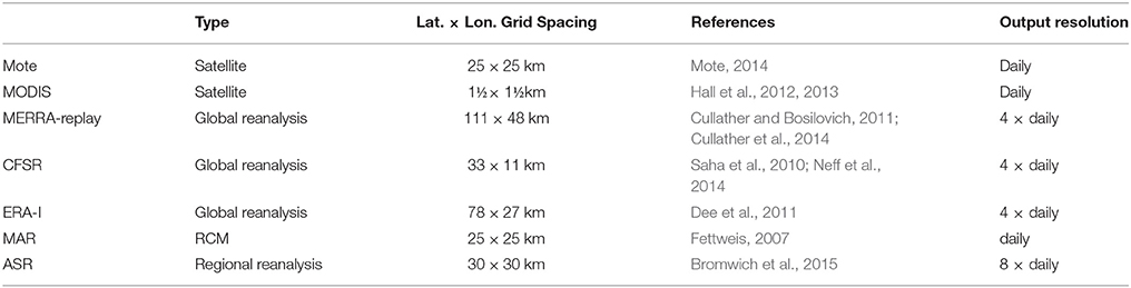
Table 1. List of data sets examined in this study.
The NASA MEaSUREs program (Making Earth System data records for Use in Research Environments) Greenland Surface Melt record (Mote, 2014) indicates the presence of water based on changes in the microwave emission detected by satellite-borne radiometers conveyed as brightness temperatures. At microwave frequencies, the emissivities of water and ice differ markedly due to differences in the respective dielectric constants. Modeling of microwave emission suggests penetration depths of a few cm's to m's depending on snowpack conditions, with a colder, dryer snowpack generally having longer penetration depth (Surdyk, 2002; Ashcraft and Long, 2006). The Mote data set uses a brightness temperature threshold determined by emission modeling for the 19 GHz horizontally-polarized channel aboard polar-orbiting Defense Meteorological Satellite Program (DMSP) platforms (Mote, 2007). The DMSP Special Sensor Microwave Imager/Sounder (SSMIS) instrument has a footprint of 47 × 73 km at 19 GHz, with twice-daily equatorial local overpass. The Mote data are made available daily on the 25 km Equal-Area Scalable Earth Grid, version 2 (EASE 2) (Brodzik et al., 2014).
An additional satellite-derived record of surface melt area used in this study was produced from NASA EOS (Earth Observing System) Terra satellite-derived ice surface temperatures from the Moderate Resolution Imaging Spectroradiometer instrument (MODIS) (Hall et al., 2012, 2013). The temperature for a skin layer of less than 2 μm thickness was retrieved in swath data within ±3 h of 1400 local solar time (1700 UTC), and a threshold of −1°C was subsequently applied to determine melt extent. The threshold value compensates for a cold bias in MODIS-derived surface temperatures (Wan et al., 2002). The retrieval is only available in clear-sky conditions, which were determined using the standard MODIS 1 km cloud mask and by manual inspection (Hall et al., 2013). The data are available daily on a 1.5 km polar stereographic grid.
Available sources of large-scale runoff are related to the use of atmospheric analyses, which assimilate observations to produce a uniformly-gridded depiction of the atmospheric state. The term “reanalyses” refers to products that assimilate data in a retrospective manner, using a consistent assimilating model to render an amount of homogeneity to the record (Trenberth et al., 2008). Typically, reanalyses assimilate state and dynamical variables while the background model produces fields of short-term prognostic variables such as cloud properties, radiative fluxes, precipitation, and surface hydrology (Kalnay et al., 1996). In these models, the surface representation of the GrIS varies considerably. Described below are three global reanalysis products which are used in this study. Also described below are a regional climate model (RCM) and a regional reanalysis, where global reanalyses are used as lateral boundary conditions.
The MERRA global atmospheric reanalysis is described in Rienecker et al. (2011), and its representation over the GrIS is examined in Cullather and Bosilovich (2011, 2012). The configuration of the system allows for the background model—the Goddard Earth Observing System model, version 5 (GEOS-5)—to be carried in phase space through analyzed states via the computation of analysis increments, a capability referred to as “replay” (Mapes and Bacmeister, 2012). For this study, a MERRA-replay is examined on a 1° × 1¼° grid. The model formulation used in the MERRA-replay utilizes the ice sheet surface representation described in Cullather et al. (2014), which allows for fractional snow cover, a prognostic surface albedo based on Greuell and Konzelmann (1994), and surface hydrology. The model represents energy conduction properties of the upper 15 m of glacial ice, and energy and hydrologic properties of an overlying, variable snow cover. Represented hydrologic processes include snow compaction, meltwater percolation and refreezing, and runoff. Firn of density greater than 500 kg m−2 is not explicitly represented.
The U.S. National Centers for Environmental Prediction (NCEP) Climate Forecast System Reanalysis (CFSR) (Saha et al., 2010; Neff et al., 2014) was produced at T-382 spectral resolution, and was obtained on a 0.3° × 0.3° grid. Prognostic fields are produced from coupled atmosphere-ocean model forecasts initialized with the data assimilation fields. The CFSR uses the Noah land surface model (Koren et al., 1999; Ek et al., 2003; see also Hines and Bromwich, 2008), which includes four prognostic subsurface layers and represents snow compaction and runoff processes.
The European Centre for Medium-Range Weather Forecasts (ECMWF) Re-Analysis Interim product (ERA-I) (Dee et al., 2011) is produced at T-255 spectral resolution, and has been obtained on a 0.7° × 0.7° grid. Flux and other model-derived fields are produced from forecasts initialized by four-dimensional variational data assimilation (4D-Var). In the ERA-I, snow density is assumed to be constant with depth. Snow depth is restricted to 0.07 m over glaciated surfaces (ECMWF, 2007). Snow albedo is parameterized after Douville et al. (1995) and is based on snow age.
The Modèle Atmosphérique Régional version 3.2 (MAR) is a RCM that utilizes the Gallée and Schayes (1994) atmospheric model. MAR uses a surface configuration described by Fettweis (2007) and Fettweis et al. (2011). MAR uses components of the CROCUS snow hydrology model (Brun et al., 1992) for the representation of snow metamorphism, melt, water percolation and refreezing, and a prognostic snow albedo. The model was integrated over a GrIS-centered domain at 25 km grid spacing, and forced at the lateral boundaries and the ocean surface with ERA-I values.
The Arctic System Reanalysis version 1 (ASR) (Bromwich et al., 2015) utilizes the Weather Research and Forecasting regional atmospheric model version 3.3.1 (WRF) adapted for polar conditions. The ASR uses the WRF 3D-Var data assimilation scheme to incorporate available satellite and in situ observations. The model was forced at lateral boundaries by ERA-I and integrated on a pan-Arctic domain at 30 km grid spacing. The ASR also uses the Noah land surface model, but with modifications for polar regions described in Hines and Bromwich (2008) and Hines et al. (2011). Specifically, the surface energy budget computation was simplified to account for differences between the boundary layer air temperature and the surface skin temperature, energy conductivity through a deep snowpack was resolved into multiple prognostic layers, and the surface longwave emissivity was increased. Notably, the NOAH land surface model used in the ASR does not have a contingency for meltwater percolation or refreezing.
Comparison of reanalysis melt area with satellite data sets is partly hindered by the available output fields of the models. Modeled daily melt area is computed here by masking for locations where the simulated maximum surface skin temperature is equal to or greater than 0°C. This reflects the method implemented for the MODIS data set (Hall et al., 2009). Obtained output fields from MAR do not contain a daily maximum skin temperature, however Fettweis et al. (2011) previously identified a simulated meltwater production rate of greater than or equal to 8.25 mm water equivalent (w.e.) day−1 as denoting melt area. Meltwater production is not an output variable of the other models. This method has been retained for computing melt area for MAR in this study.
For this study, variables are examined over the full ice sheet, but also over major drainage basins defined by Zwally et al. (2012) and indicated in Figure 1. Numerous studies have found the GrIS to be spatially heterogeneous, and that local climate and geometry influence mass balance parameters on the basin scale (e.g., Vernon et al., 2013; Andersen et al., 2015; Seo et al., 2015). For comparison, model fields have been interpolated to a common grid using a tension spline interpolation algorithm (Renka, 1997). As inadequate spatial resolution has been identified as an important issue in representing observed melt processes (Ettema et al., 2009), the Mote data set 25 km EASE-2 grid was selected as the coarsest resolution of the two satellite records. The analysis is conducted for the available summer melt season (May to September) in the 13-year overlapping period of the satellite and model data sets, which is 2000-2012.
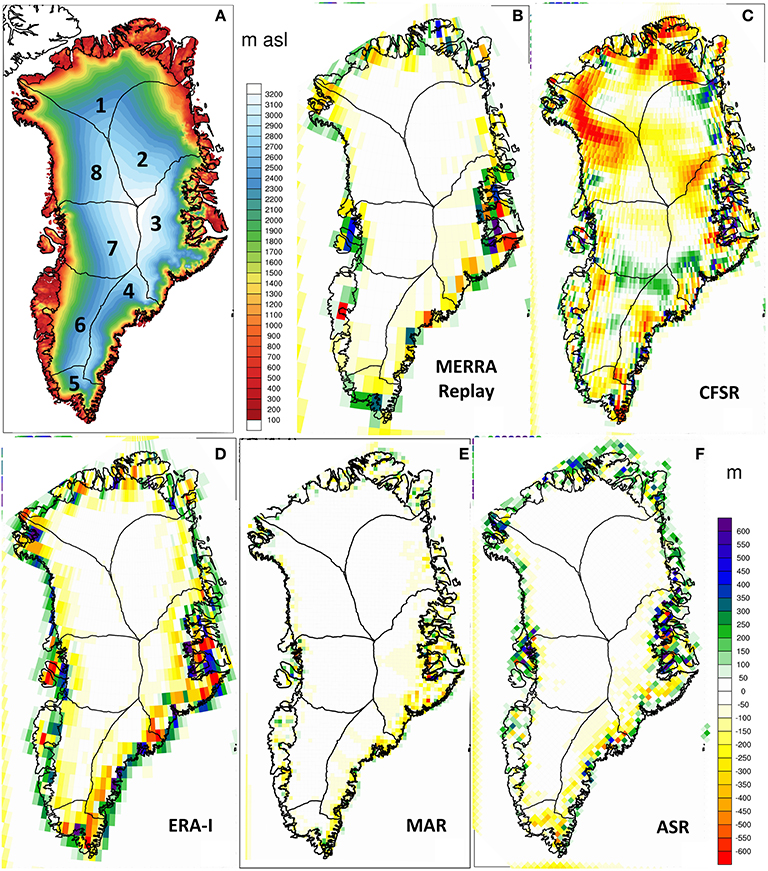
Figure 1. (A) Greenland surface elevation from Bamber et al. (2001) contoured every 100 m asl, and differenced with (B) MERRA-replay (C) CFSR, (D) ERA-I, (E) MAR, and (F) ASR, in m. The major GrIS drainage basins of Zwally et al. (2012) are numbered in (A) and indicated in each difference plot.
Results
Topography and Annual Mean SMB
An adequate topographic representation of the ice sheet is an important consideration in modeling surface conditions. Figure 1A presents the widely-used Bamber et al. (2001) topographic data set, which is based on satellite radar altimetry. Figure 1 also shows the difference in topography for each model examined compared with the reference (Bamber et al., 2001). The models have incorporated modern GrIS topography estimates to some extent with the notable exception of the CFSR (Figure 1C), which used the outdated U.S. Geological Survey global 30 arc-second elevation data set (GTOPO30) that is known to have significant errors (Box and Rinke, 2003). Apart from the baseline reference source, differences may result from other considerations including the treatment of gravity wave drag, spatial resolution, and gridding requirements. Several of the models indicate an underestimate in elevation along the steep ice sheet escarpment in the southeastern GrIS, and the difference plot for the ERA-I (Figure 1D) presents a pattern of negative and positive values parallel to the coast that is characteristic of the Gibbs phenomenon in spectral models (Hoskins, 1980). Discrepancies are also shown in some models for non-glaciated locations where available sources for the Bamber et al. (2001) data set were limited.
MERRA-replay, ERA-I, CFSR, MAR, and ASR comprise a spectrum of contemporary sources for recent GrIS historical surface runoff information. A brief overview of this range may be obtained from the time series of GrIS SMB components shown in Figure 2 for the years 2000-2012, and time-averaged values are shown in Table 2 for the full GrIS and major drainage basins as defined by Zwally et al. (2012) and indicated in Figure 1. Note that negative evaporation values in Table 2 for MAR denote net deposition, which has been observed at GrIS high elevation locations (Box and Steffen, 2001). Hanna et al. (2005) and Vernon et al. (2013) previously found that estimated GrIS SMB is poorly constrained, and the models shown here support that conclusion. The cross-model standard deviation of SMB is 41% of the median value, which is similar to the results of Vernon et al. (2013). For drainage basins in the south and southwest, the multi-model spread in SMB is larger than the median value. Among SMB components for the GrIS, discrepancies in runoff are much larger than for precipitation. The GrIS multi-model standard deviation for runoff is 45% of the median value as compared with 13% for precipitation. Similar discrepancies are found for each basin, and it may be seen in Figure 2 that differences in annual values and trend in SMB are largely reflected by changes to the runoff. The multi-model uncertainty in SMB components has an important bearing on the interpretation of recent trends. Using a RCM, Seo et al. (2015) found SMB trends over the last decade were largely associated with decreased precipitation until the melt events of 2010 and 2012. For the period shown in Figure 2, the trend in annual precipitation among the five models ranges from −6.0 to −15.8 Gt yr−1, while the trend in runoff varies from 2.9 to 34.7 Gt yr−1. For the MERRA-Replay, MAR, and ASR models, the magnitude of the trend in runoff is larger than that for precipitation, while the reverse is found for the CFSR and ERA I. This is reflected in the interannual standard deviations which are shown in parentheses in Table 2. The interannual standard deviations for GrIS runoff are typically 24% of the mean value for each model, while the standard deviations for precipitation are 10%.
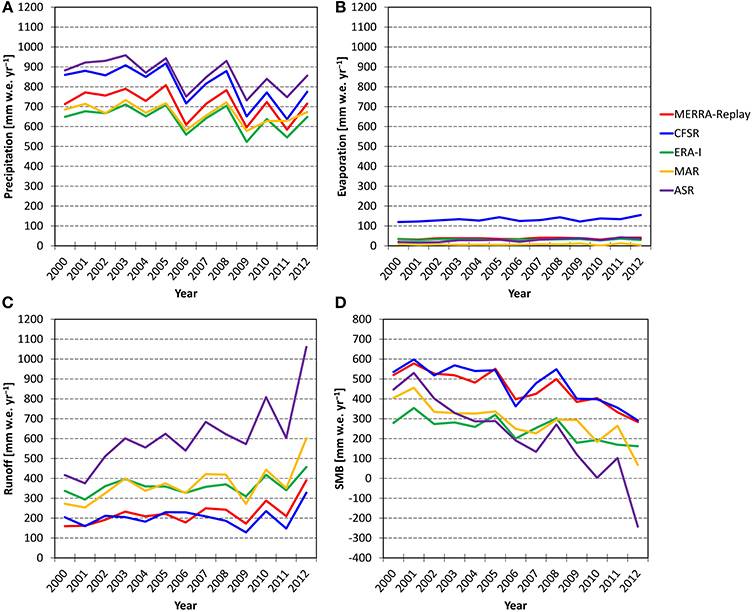
Figure 2. Time series of annual (A) precipitation, (B) evaporation, (C) runoff, and (D) SMB averaged over the GrIS from five data sources, in mm water equivalent (w.e.) yr−1.
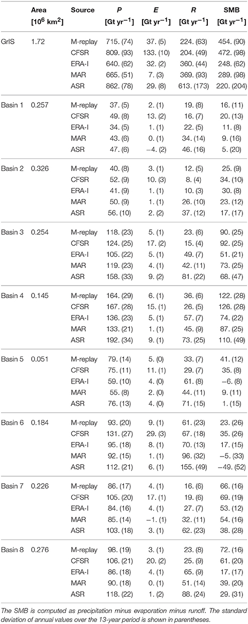
Table 2. Precipitation (P), evaporation (E), runoff (R), and computed SMB for the GrIS and drainage basins as defined by Zwally et al. (2012) from five models for the period 2000-2012, in Gt yr−1.
Evaluation of Satellite Data Sets
Differences between the two satellite-derived data sets are briefly examined. A more comprehensive evaluation is beyond the scope of this paper and may be found elsewhere (e.g., Ashcraft and Long, 2006; Tedesco, 2007; Hall et al., 2009; Nghiem et al., 2012; Tedesco et al., 2015). For purposes of this study, the major differences are identified in order to characterize uncertainty when comparing against model fields.
Figure 3 shows the 2000-2012 average number of melt days per year on the GrIS and the difference between the two satellite-derived data sets. The respective data set resolutions may be distinguished from a visual inspection of Figures 3A,B: the larger grid size (25 km) for the Mote data is clearly evident, while MODIS has a much finer resolution (1.5 km grid spacing). Similar to Hall et al. (2012), the color scale for Figures 3A,B emphasizes the extent of persistent summertime melt in each data set, with a sharp contrast between the areas of melt days greater than 20 along the ice sheet periphery and interior regions where values are generally less than 10 days. The two data sets generally agree in showing persistent seasonal melt along all peripheral sides of the ice sheet, but extending disproportionately further inland from the southwestern margins. For MODIS, there is the additional issue of missing data due to cloud cover. The MODIS values are extrapolated by using the ratio of available observations for the available period 1-May through 30-September. The average number of observing days available, shown in Figure 3C, decreases from close to 90% over the northeast GrIS to under 50% in the south where clouds are more prevalent. MODIS indicates less than one melt day on average for a broad area of the GrIS plateau, while Mote indicates up to 3 days over a similar area. This difference is likely indicative of cloud cover, which can produce surface warming over the ice sheet interior while obstructing MODIS observations of individual melt events occurring at higher elevations.
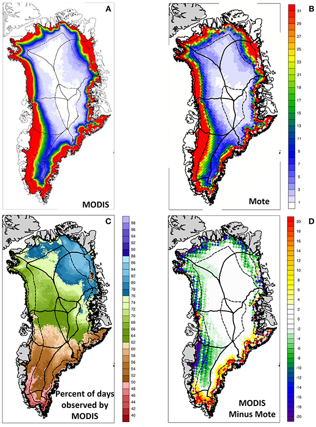
Figure 3. Average number of GrIS melt days per year derived from (A) MODIS surface temperatures and (B) passive microwave data using the algorithm of Mote (2007) for 2000-2012. MODIS values were extrapolated based on the available number of observing days. (C) The percentage of days observed by MODIS. (D) Difference of the average number of melt days derived by MODIS minus passive microwave data using the Mote (2007) algorithm. Boundaries of major GrIS drainage basins of Zwally et al. (2012) are indicated, and surface orography from Bamber et al. (2001) is indicated with dashed contours for every 1000 m of elevation.
The difference of the two averaged fields shown in Figure 3D reveals a characteristic pattern where the number of melt days for MODIS is generally greater than for Mote in the southeast– extending from the Scoresby Sund down to the GrIS southern tip, while the average number of melt days in the Mote data are greater elsewhere along the ice sheet edge. Along the western periphery, the difference in the number of melt days extends to higher elevations. For example, the Mote data set has an average of 2–6 more melt days per year in close proximity to the divide between drainage basins 4 and 6 over the southwestern GrIS. The reason for these difference patterns are not known, but some inference may be obtained from the location and the limitations of the instruments. In the southeast, microwave brightness temperatures may be affected by large topographic gradients within the pixel or by metamorphic snow grain changes, such as surface hoarfrost formation along the coastal escarpment due to temperature gradients and subsequent destruction by wind. On the periphery of the southeastern GrIS, high precipitation and melt also allow water to percolate to depth, both warming the snow/firn and altering the emissivity of the firn column at depth (e.g., Koenig et al., 2014). All of these processes could affect the microwave brightness temperature without changing the surface temperature recorded by MODIS. Alternatively, the southeast is also associated with significant cloud cover; MODIS coverage in these areas is typically less than 60 percent as seen in Figure 3C.
Some additional insight may be obtained by examining the temporal variability. It is found that greater than 95% of the ice sheet is observed by MODIS over a centered 5-day window. In Figure 4, the time series of daily Mote passive microwave is shown in comparison to MODIS 5-day observations. For direct comparison, the 5-day average of the Mote passive microwave data is also plotted. For the entire GrIS shown in Figure 4A, the Mote passive microwave data and the MODIS data are very similar on 5-day time scales. MODIS tends to have a larger melt area than Mote passive microwave in transitional seasons but slightly less than the Mote data during peak melt. There is also similar agreement for the extreme melt year 2012 shown in Figure 4B as with the long-term average. Again, MODIS melt area tends to be larger at the beginning and the end of the melt season, while the Mote data tends to show larger melt area in late June and July. For the 5-day period centered on the time of maximum melt occurring on 11-July 2012, the MODIS-derived melt area is found to be 1.17 × 10⁶ km2 while the corresponding Mote passive microwave-derived melt area is 1.28 × 10⁶ km2. The discrepancies between the data sets are consistent with the previous inference that passive microwave data have some difficulty observing melt confined to the edges of the ice sheet associated with variable topography, and that cloudiness may interfere with MODIS sensing the entirety of a large melt area during the time of maximum melt.
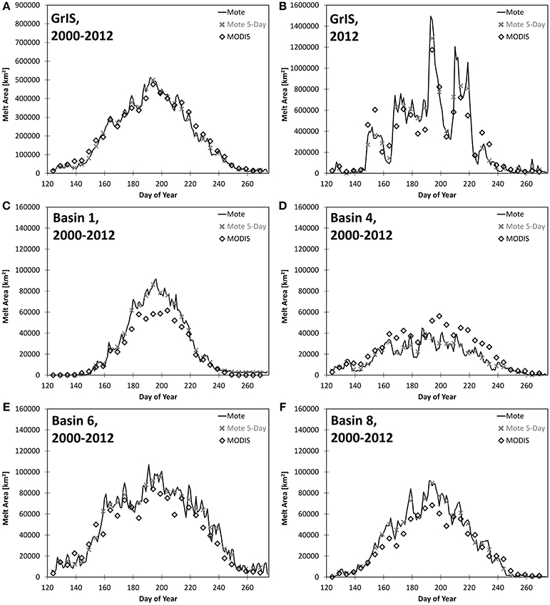
Figure 4. Annual time series of melt area derived from passive microwave (solid line) and MODIS 5-day averages (diamonds), in km2. Passive microwave 5-day averages corresponding to the MODIS values are indicated with an “×.” Time series are indicated for (A) the total GrIS, averaged for 2000-2012; (B) the total GrIS for the year 2012; and (C) drainage basin 1, (D) basin 4, (E) basin 6, and (F) basin 8 averaged for 2000-2012.
The spatial differences in the number of melt days shown in Figure 3D may be further investigated using the melt area time series for selected drainage basins shown in Figures 4C–F. For basin 4 in the southeast, the MODIS-derived melt area is consistently greater than the Mote passive microwave value over the melt season, which is in agreement with the difference in the number of melt days shown in Figure 3. For basin 6 in the southwest GrIS, it may be seen that the daily Mote passive microwave time series shows considerable variability, even when averaged over 13 years. For this basin, the full time series is characterized by individual events of large amplitude. The MODIS melt area is generally less than the Mote passive microwave values. Again, intermittent cloudiness may interfere with MODIS sensing large melt areas associated with these events. The melt area may also be preferentially enhanced under cloudy conditions due to longwave radiative forcing (e.g., Bennartz et al., 2013). For basin 1 in the northern GrIS, cloud cover is less frequent, and here the differences in the number of melt days and the melt area for the two satellite data sets are not immediately discernible.
Figures 3, 4 also illustrate the basin-to-basin variability in the character of the melt season. The calendar day of maximum melt varies by basin, and is generally earlier in the season in the southeast. This is potentially due to the availability of open-water surface heat fluxes from the adjacent ocean in the south and onshore heat advection from the North Atlantic storm track. Other regions of the GrIS—particularly in the north—are adjacent to ice-covered seas later into the season. Figure 4 also indicates that the timing and duration of the average melt season varies by basin. From the Mote passive-microwave data, significant melt in northern basin 1 is seen to begin on day 150 (30-May) and end on day 240 (28-August). For basin 6, the melt season begins on day 120 (30-April) and ends on about day 250 (7-September). Further indications of the differing conditions of the basins are seen in the day-to-day variability in Mote passive-microwave melt area in the time series shown, which increases southward. As mentioned above, this is indicative of individual melt events of large area occurring on sub-seasonal time scales, which distort the 2000-2012 averaged time series. For the full 2000-2012 daily time series (not shown), there is good correlation in the Mote passive microwave melt area between adjacent drainage basins in the north and the south. With no lead or lag, the time series for basins 1 and 2 have a correlation of r2 = 0.71 and basins 5 and 6 have a correlation of r2 = 0.69, while for basins 2 and 5, r2 is 0.13. The lead/lag in maximum correlation between basins generally does not exceed 1–2 days, with basin 2 in the northeast lagging western basins.
Comparison of Model Melt Area
Figure 5 shows the mean spatial pattern of melt days for five models for the years 2000-2012. The ASR can be seen to be an outlier in showing more melt days within the interior, and a longer melt season in the southern half of the ice sheet. Among the other four models, there is general agreement in the extent of the melt season on the western and south-eastern periphery. In contrast to satellite observations (Figure 3), the other models indicate no melt days over the 2000-2012 period for the interior GrIS at elevations greater than 2500 m asl, with the exception of the CFSR and ASR. The CFSR may be expected to have more melt days as a result of its use of a lower topography.
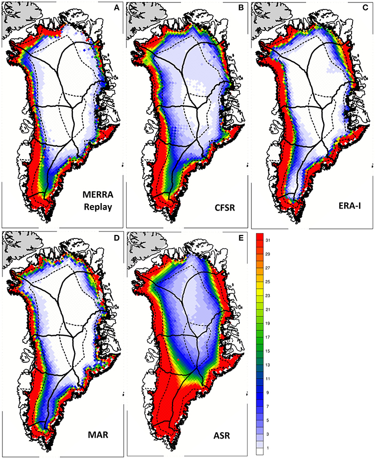
Figure 5. Average number of GrIS melt days per year for (A) MERRA-replay (B) CFSR, (C) ERA-I, (D) MAR, and (E) ASR. Boundaries of major GrIS drainage basins of Zwally et al. (2012) are indicated, and surface orography from Bamber et al. (2001) is indicated with dashed contours for every 1000 m of elevation.
Two areas of marked disagreement among the models are in the interior of the southern part of the ice sheet and in the northeastern GrIS. For drainage basin 6 in the southwestern GrIS, the models largely concur in identifying the region of seasonal melt (i.e., greater than 28 days) as extending inland to an elevation of approximately 2000 m asl, which is in rough agreement with the field shown in Figure 3A for MODIS data. But for the region of transitional melt further inland, there is greater disagreement. For example, the average number of melt days for the interior of the southern part of the GrIS in the models varies from less than 2 for the ERA-I to greater than 30 for the ASR, while the satellite data sets agree on 5–7 days. In the northeastern GrIS, MAR and ERA-I show large areas of melt lasting 30 days or more that extend further inland than the other models, while the MERRA-Replay and CFSR indicate melt of 10 days or less adjacent to Peary Land and the Danmark Fjord. However, none of the models capture the inland extent of the persistent melt region as seen in the observations in basins 1–2.
Further insight into the relative spatial differences may be examined with the use of Taylor diagrams (Taylor, 2001). Taylor diagrams use metrics of spatial correlation and standard deviation to compare model patterns to a reference data set. Spatial correlation shows the degree to which patterns match a reference data set, while standard deviation compares the amplitude of the spatial variations. With the standard deviation normalized to the reference data set, proximity to the (1, 1) coordinate location in the diagram presents the relative skill of the model to reproduce the reference spatial pattern (e.g., Bosilovich et al., 2008). The linear distance from the origin coordinate indicates the area-weighted root-mean-square (RMS) error from the reference data set, after removing the means. The Taylor diagrams shown in Figure 6 present a comparison of the fields plotted in Figures 3, 5 for each basin. The diagrams shown vary substantially based on the reference satellite observation. In addition, the satellite data sets compare with each other only slightly better than with the models, as large differences are apparent. There is considerable spread in the spatial correlation of the models to the observation for both reference datasets, from less than 0.7 to ~0.99. There also considerable spread in the ratio of standard deviation. In general, the basins for ERA-I have higher spatial variance and are further from the (1, 1) reference. Basin melt days shown for the MAR model have lower variance and high spatial correlation and hence lower RMS, and the other models generally fall in between.
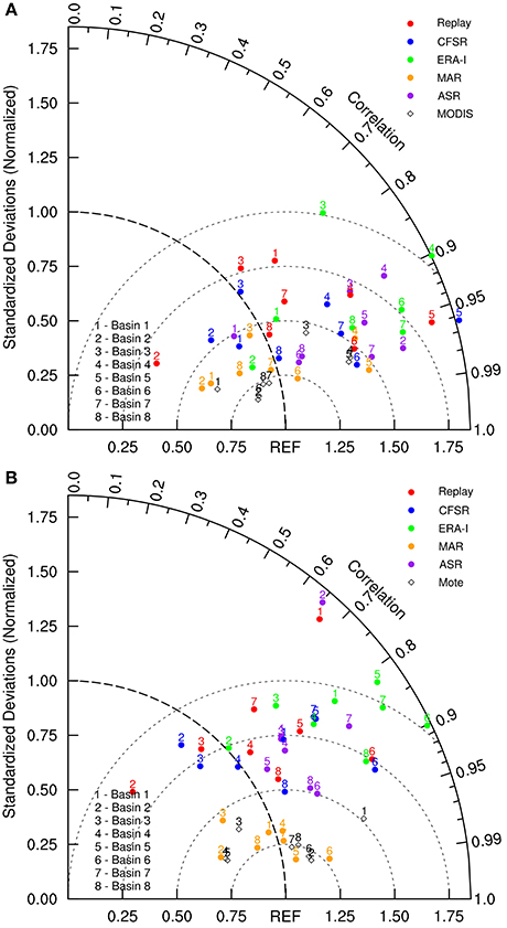
Figure 6. Taylor diagrams of number of melt days for indicated drainage basins for (A) relative to passive microwave data and (B) relative to MODIS data.
Interestingly, no basin is uniformly favored for all models, and the Taylor diagrams initially appear highly chaotic. This suggests that each model has unique preferential locations for comparison to the satellite data sets. Nevertheless, one may see that the normalized standard deviation for basins 1 and 2 are less than unity for a majority of the models referenced to Mote, and that the normalized standard deviation for basin 3 is less than unity for the MODIS referenced diagram. This indicates that, in general, the models have less spatial variance than observed for the northern and northeastern basins, and this is readily apparent from Figures 3, 5.
One may use the Taylor diagrams to identify the individual basins for each model that compare most favorably to the spatial patterns of melt days determined from the satellite data. For global reanalyses, northern basins are in relatively closer proximity to the unity point for both Mote and MODIS than the other basins. The MERRA-replay and the CFSR both compare with satellite data best for northwestern basin 8, while the ERA-I comparison is most favorable for northeastern basin 2. For the RCMs, the southern basins 6 and 7 are better reproduced based on the Taylor diagrams. This implies that the coarser-resolution models preferentially perform better for basins in which the number of melt days is more uniform over the basin, while higher-resolution RCMs preferentially perform better in the regions of a longer melt season in the south. The basins in the south also tend to have a stronger spatial gradient in the number of melt days, and the higher resolution models preferentially perform better in basins with these conditions. Again, there is considerable overlap among the models in terms of performance, with a more favorable comparison to Mote than to MODIS. Among global reanalyses, a general conclusion that higher resolution models outperform those with coarser grid spacing for all basins is not supported.
The temporal evolution of melt area provides an additional perspective of the representation of melt seasons in the models (Figure 7). For the total ice sheet area, the ASR is again an outlier and exceeds satellite estimates by as much as 300,000 km2. The MAR model generally indicates a smaller melt area than satellite data for the full GrIS, and particularly for the second half of the melt season. Among the other models, the ERA-I indicates greater melt area than the satellite data sets and the other two global reanalyses for the first half of the season. In the second half of the season, the CFSR, ERA-I, and the MERRA-replay closely agree with each other, but indicate greater melt area than the satellite data sets by about 50,000 km2. The range of values among the models is larger than the differences between the two satellite data sets. The models agree with satellite data in showing the maximum melt extent occurring on approximately day 195 (14-July).
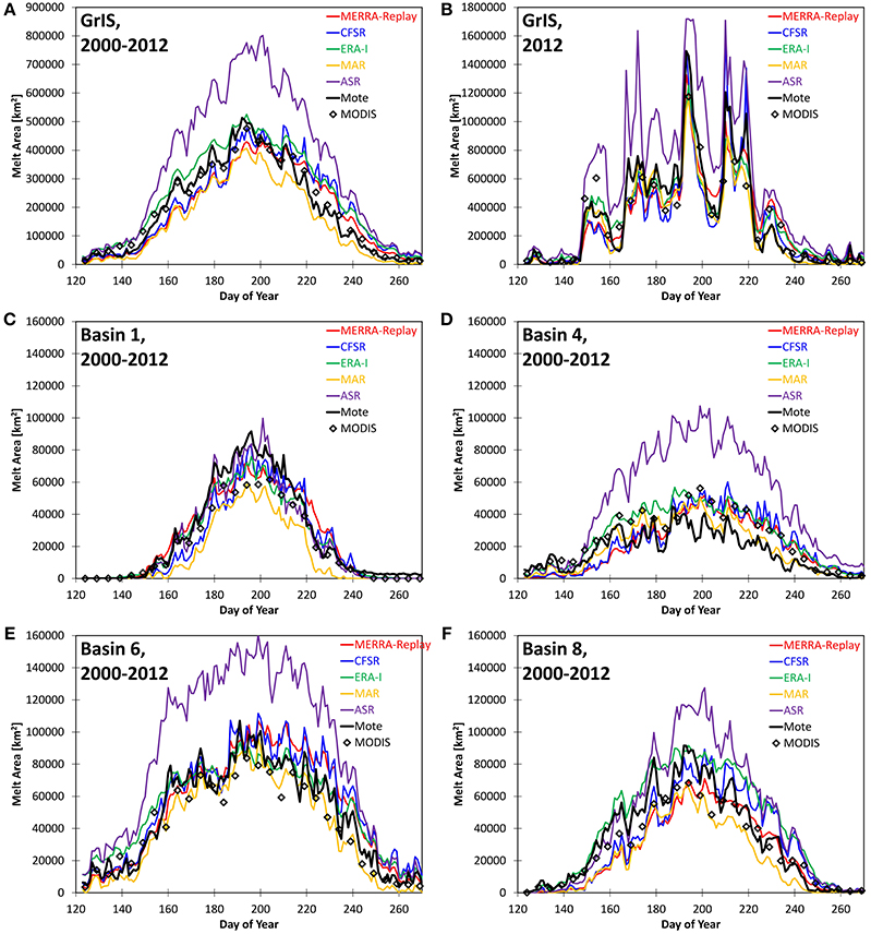
Figure 7. Annual time series of melt area from five data sets in comparison to passive microwave (solid black line) and MODIS 5-day averages (diamonds) for (A) the total GrIS, averaged for 2000-2012; (B) the total GrIS for the year 2012; and (C) drainage basin 1, (D) basin 4, (E) basin 6, and (F) basin 8 averaged for 2000-2012, in km2.
For the individual year of significant melt in 2012 shown in Figure 7B, it may be seen that there is good correlation among the models and satellite data sets in reproducing the time series of individual melt events. For the maximum melt event on 11-July, four of the models are within the range suggested by the satellite data. For the year 2012, the melt extent shown for ASR is again persistently greater than for the other models and the satellite data sets. As with the 2000-2012 average, there is greater disagreement in the transitional seasons. For the time series of selected individual drainage basins shown in Figures 7C–F, it may be seen that the overestimate of GrIS melt extent for the ASR primarily occurs in regions in the central and southern areas of the GrIS, while the ASR time series for basin 1 in the northern GrIS is notably closer to that derived from Mote passive microwave data. For basins 1 and 8, the MAR model indicates a smaller melt extent than for the other models over the time series. It is only during the peak melt season that the melt area in MAR is comparable to the MODIS-derived melt extent for basins 1 and 8, which is still less than that found for the Mote passive microwave. It may be seen from the spatial maps in Figures 3, 5 that the region of persistent melt in the western areas of basin 1 occupies a more peripheral region in MAR than for the other models and for the satellite data sets, in agreement with the differences seen in the time series and the Taylor diagrams. The basin-scale time series shown in Figure 7 indicates that global reanalyses preferentially agree with the larger estimate of the two satellite data sets: for basin 1, the reanalyses melt areas tend to agree more closely with the Mote data in showing larger areas at the peak of melt season; for basin 4, the reanalyses agree more closely with MODIS-derived melt area over the course of the melt season. An exception is drainage basin 8, where the global reanalyses have a large range of estimated melt area. The melt area from the CFSR and MERRA-replay are less than for the two satellite data sets during the first half of the melt season, while the ERA-I indicates periods where values are larger than the satellite-derived melt area.
Comparison of Model Runoff
The spatial distribution of annual mean runoff is shown for the period 2000-2012 from the five models in Figure 8. The models agree in indicating runoff along the edges of the ice sheet with larger values occurring along the southern periphery. In comparison to melt zones that are highlighted in Figure 5, significant runoff volume is found to occur exclusively at the very margins of the ice sheet in the models. The ASR indicates runoff of greater than 100 mm w.e. yr−1 over the inland areas of the southern part of the GrIS that is not found in the other models, but GrIS runoff in the ASR is not in substantial disagreement with the range of spatial distributions shown for the other models, as was the case with melt area shown in Figure 5. Nevertheless, the range of spatial distributions for the models is considerable. In the MAR regional model and the ASR regional reanalysis, particularly large runoff volume of greater than 1800 mm w.e. yr−1 is found to occur in the southwestern and western GrIS, while the global reanalyses suggest more balance between the southeastern and southwestern GrIS. The two high-resolution regional models in fact suggest large runoff values along the entirety of western ice sheet periphery. While there is more balance in southeastern and southwestern runoff, the CFSR indicates less runoff in the southeastern GrIS—less than 800 mm w.e. yr−1—than is found in the other models. The ERA-I indicates values greater than 1800 mm w.e. yr−1 in northwestern Greenland near Thule while runoff in other models is less than 1000 mm w.e. yr−1 for that region.
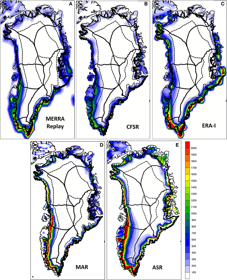
Figure 8. Average surface runoff per year for 2000-2012 for (A) MERRA-replay (B) CFSR, (C) ERA-I, (D) MAR, and (E) ASR, in mm w.e. yr−1. Boundaries of major GrIS drainage basins of Zwally et al. (2012) are indicated, and surface orography from Bamber et al. (2001) is indicated with dashed contours for every 1000 m of elevation.
As suggested by the spatial patterns, the time series of runoff for the models shown in Figure 9 are disparate. In agreement with Table 2, the ASR time series shown in Figure 9 indicates more runoff volume than for the other models for the entire GrIS and for each basin. In Figure 8, it was seen that the spatial distribution of ASR runoff is not substantially different from the range of spatial distributions found in other models. This suggests that the larger runoff in the ASR as compared with the other models originates from similar peripheral locations, rather than runoff occurring over a larger spatial area. It is also noted from Table 2 that precipitation volume is larger in the ASR than for the other models, and this may play a role in supplying runoff volume in the model. The MAR regional model is found to provide the second-largest runoff for the GrIS and for selected basins shown in Figure 9. However, as seen in Table 2, the runoff from global reanalysis ERA-I is larger than for the regional model MAR for basins 3, 4, 5, and 8. The CFSR reanalysis generally has the smallest runoff volume for the GrIS and for basins 1 through 5. The time series shown in Figure 9 indicate several points of disagreement among the models. The day of maximum runoff in the ASR is earlier than for the other models, particularly for the whole GrIS (Figure 9A) and basin 1 (Figure 9C). The runoff for MAR indicates a much smoother time series for the GrIS and for individual basins. This is particularly evident for the individual year 2012 shown in Figure 9B, but also for other individual years (not shown). The daily variations are larger in time series for the other models and are suggestive of the melt area time series shown in Figure 7. Over the 2000 to 2012 time period, the daily runoff in MAR in fact has a lower correlation with melt area (r2 = 0.805) than for the other models. The MAR runoff is larger in the second half of the melt season, while the global reanalyses are generally more symmetric about the melt season. A notable exception to this the extended runoff season suggested by the ERA-I. The runoff in ERA-I extends into the autumn season while the other models generally agree on the seasonal cessation of runoff.
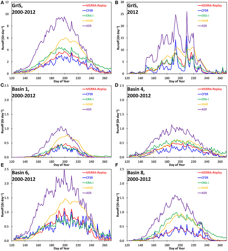
Figure 9. Annual time series of runoff from five data sets for (A) the total GrIS, averaged for 2000-2012; (B) the total GrIS for the year 2012; and (C) drainage basin 1, (D) basin 4, (E) basin 6, and (F) basin 8 averaged for 2000-2012, in Gt day−1.
It is useful to examine the nature of the relation between runoff and melt area in the surveyed models. In the absence of an observed association between large-scale melt area and runoff, Reeh (1991) suggested that the relation between summer near-surface air temperatures and melt volume is of the form of a third-order polynomial. Summer temperatures relate to melt area in a manner that is dependent on basin geography. Subject to basin geography, the relation between melt area and runoff may be plausibly expected to reflect a lower-order polynomial in the absence of more complex feedback processes.
Figure 10 shows the scatter diagram of runoff volume vs. melt area for the models for the GrIS and for selected basins. For each basin, runoff is found to monotonically increase with increasing melt area. A weak polynomial relation may be seen as an acceleration of runoff for increasing melt area in selected basins, most notably in basin 6 (Figure 10E). The relation for the total GrIS shown in Figure 10A indicates greater runoff per unit melt area for the MAR and ASR regional models. The figure indicates hysteresis for these two models, in that relation of runoff to melt area differs between the first half of the melt season and the second half. For the ASR, these differences are more discernible over periods where the melt area is less than 0.40 × 10⁶ km2. Hysteresis originates from the timing of runoff shown in Figure 9 in which the MAR runoff is larger in the second half of the season, the ASR runoff is larger in the first half of the season, and the global models are more symmetric in the temporal evolution of runoff. For MAR, this hysteresis is found to occur in all basins. Runoff in the second half of the season is particularly large per unit area. For individual basins, the slope of the MAR and ASR exceeds that of the global models for basins 1 and 8 in the northern region of the GrIS, while the ratio is comparable for the regional and global models for basins in the south of the GrIS.
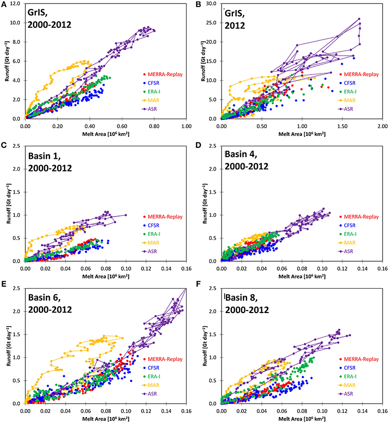
Figure 10. Daily runoff in Gt day−1 vs. melt area in 106 km2 from five data sets for (A) the total GrIS, averaged for 2000-2012; (B) the total GrIS for the year 2012; and (C) drainage basin 1, (D) basin 4, (E) basin 6, and (F) basin 8 averaged for 2000-2012, in Gt day−1. Connecting lines for MAR and ASR values indicate the progression of the seasonal cycle.
The scatter of averaged daily values of runoff and melt area for each model is shown in Figure 11. The models exhibit remarkably different relations between runoff and melt area. For example, the CFSR indicates substantial continuity in the ratio, while individual basins are more clearly discernible for the MERRA-replay and the ERA I. The ERA-I in particular suggests a separation of basins with a higher ratio of runoff to melt area in the southern GrIS (basins 4, 5, 6) from basins in the north with a lower ratio. Basin 4, which is located in the southeastern GrIS, is seen to have a larger ratio of runoff to melt area as compared to other drainage basins for the MERRA-replay. For other models such as the ASR, the ratio of runoff to melt area for basin 5 is less than that found for other models. For MAR, the hysteresis in the ratio as described earlier is apparent in all basins.
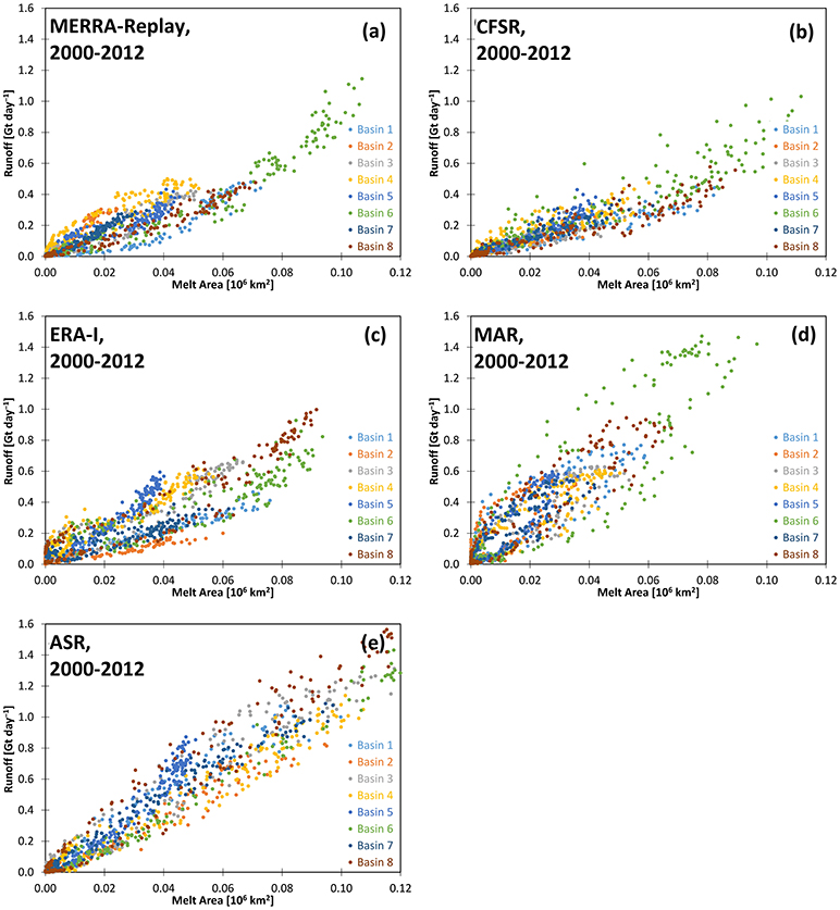
Figure 11. Daily runoff in Gt day−1 vs. melt area in 106 km2, averaged for the period 2000-2012 from (A) MERRA-replay (B) CFSR (C) ERA-I, (D) MAR, and (E) ASR.
Discussion
Historical GrIS melt area and runoff volume produced from three global reanalyses, a RCM, and a regional reanalysis have been analyzed for the period 2000-2012. Derived melt area compares favorably with two satellite-derived products, with notable exceptions in the interior regions of the southern part of the ice sheet and in the northeastern GrIS, and for the ASR. The models differ markedly on the average number of melt days at higher elevations of the southern part of the GrIS. The models also vary in the number melt days along the northeastern periphery, and are commonly less than suggested by satellite data. The models generally agree with satellite observations in the extent of the persistent melt area elsewhere on the GrIS, and there is good correlation with the daily time series of melt area. In contrast to this relative agreement in melt area, the mean values of runoff vary markedly from 204 Gt yr−1 in the CFSR to 613 Gt yr−1 for the ASR. Notably, the seasonality of runoff differs among the models. Global reanalyses suggest a symmetrical runoff season while the ASR tends to show more runoff in the earlier part of the year, and MAR indicates more runoff in the second half of the melt season. The MAR daily runoff generally shows less day-to-day variability and a lower temporal correlation with melt area than for the other models. The reasons for this difference in the temporal character are unclear. It is difficult to ascertain the differences in the surface configuration among the models from available documentation. However, it may be speculated that the overall depth of the surface representation in MAR may be considerably greater than that for other models—for example, the 0.07 m snow depth used in the ERA-I. This may result in a different amount of energy storage within the snow pack that would allow for a more extended runoff period. Differences in the represented energy conductivity of the snow pack as well as the initial conditions of deeper layers may also play a role. An examination of the relation between runoff volume and melt area indicates considerable complexity. For this relation, the surveyed models differ for the whole of the GrIS and from basin to basin. The asymmetric nature of the melt season in the ASR and MAR produces hysteresis in the runoff-to-melt area relation both on the basin scale and for the GrIS average. The direction of the hysteresis for the ASR is opposite to that for MAR.
The analysis indicates substantial uncertainty in recent, historical runoff on a variety of time scales and for different basins. As noted above, the range of mean values of runoff for the GrIS among the available sources is 389 Gt yr−1. A detailed understanding of this range of values is hindered by a lack of complete documentation of the various model configurations. Aspects that may play a role include the method of initialization for the snow pack, the complexity of snow hydrological processes represented including refreezing and meltwater percolation, and snow pack energetics including conductivity and the representation of surface albedo.
The temporal evolution of albedo may significantly contribute to uncertainty due to its important influence on melt processes. For example—early season melt, subsequent surface metamorphism, and the positive albedo feedback mechanism have been identified as critical components in GrIS melt events (e.g., Tedesco et al., 2011). The prognostic albedo scheme in the MAR RCM differs considerably from CFSR and ERA-I reanalysis parameterizations that were designed for terrestrial surfaces (Wang and Zeng, 2010). An assessment of the albedo feedback mechanism strength in each of the models is a topic for additional investigation. However, common use of the Greuell and Konzelmann (1994) albedo parameterization in MERRA-replay and in RCMs widely used for GrIS analysis (e.g., Ettema et al., 2010) suggests the added importance of interactions between the simulated albedo and other model components, such as snow hydrology or horizontal resolution. Comparisons with observed albedo records are also susceptible to difficulty (e.g., Polashenski et al., 2015).
Additional factors in runoff uncertainty include differences in atmospheric forcing conditions. This includes the amount and phase of precipitation, and the amount of cloud cover. The amount and phase of cloudiness affects surface temperatures through the partitioning of solar and terrestrial surface radiative fluxes. Differences in solar forcing may significantly affect surface melt through the albedo feedback mechanism. Mixed and liquid-phase clouds, which are difficult to correctly model (Sotiropoulou et al., 2015), also play a role in surface melt through the enhancement of downwelling longwave radiation (Bennartz et al., 2013).
The three global reanalyses considered in this study show a sizeable range in mean values of runoff, but also show relative similarity in the temporal variability for selected basins and in the relation between runoff and melt area as compared to MAR and ASR. The global reanalyses differ markedly in spatial resolution and in the representation of surface processes, including albedo. Albedo for the MERRA-replay is related to evolving snow density and fractional snow cover, while the CFSR and ERA-I are related to snow age. These configuration differences mostly cancel in order to produce similarities in temporal variability and in the runoff-to-melt area relation. This is indicative of non-linearity in the contributions of the differing model components to uncertainty.
In recent years, RCMs have frequently been applied to the examination of GrIS SMB components. RCMs are thought to provide necessary spatial resolution, and are able to incorporate locally-specific physical parameterizations to represent advanced snow hydrology and firn processes (Rae et al., 2012; Church et al., 2013). RCMs are forced with global reanalyses at lateral boundaries but are allowed to integrate freely. Careful consideration in the selection of a limited domain size and the orientation of lateral boundaries with respect to forcing circulation may allow for the RCM to provide an historical time series of surface properties (Seth and Rojas, 2003; Leduc and Laprise, 2009). MAR has been widely used for studies of the GrIS climate (Tedesco et al., 2011, 2013). Due to the constraints of the model configurations and available output fields, a meltwater threshold was applied in determining melt area for MAR as compared with the maximum daily surface temperature in the reanalyses. Fettweis et al. (2011) previously examined various methods for determining melt area from MAR output. Fettweis et al. (2011) found that while the threshold value has considerable influence on the determined melt area, the trend and variability are similar. Spatial resolution, differences in the surface representation, and the free integration mode associated with the RCM approach may all play a role in the temporal character of the daily runoff time series. A relevant question is with regards to the sensitivity of the RCM to the given global reanalysis boundary conditions. Some insight may be obtained in Franco et al. (2013), in which MAR was forced by various global models to assess projected twenty-first century changes to the GrIS. Franco et al. (2013) found the ability of global models to reproduce the surface climate constituted the largest uncertainty in future simulations of the GrIS. A similar conclusion is suggested for reanalyses, indicating the importance of global reanalysis development for RCM simulations.
The study suggests several areas of further investigation. In general, the satellite data sets agree reasonably well despite differences in the retrieval method and sampling. But differences remain in regions of steep topography and persistent cloud cover, which require resolution. The surveyed models differ substantially in physical complexity, but some conclusions may be inferred. Early season runoff as shown in the ASR suggests a relation between the accumulated snowpack and runoff. As noted previously, the NOAH land surface model used in the ASR does not have a contingency for meltwater percolation or refreezing. The late-season runoff found in MAR suggests a seasonal retention in meltwater or melt energy within the snowpack, and is perhaps related to the additional complexity of the CROCUS land surface model. Different surface forcing, such as through the prognostic surface albedo, or enhanced energy conduction may lead to a preconditioning of the snowpack to enhanced runoff in the second half of the season. It remains unclear whether hysteresis is a realistic feature of the surface runoff representation on the basin scale. Such a condition would invalidate any prescribed relation that does not account for seasonality. Reanalyses and regional models forced by reanalyses are constrained to represent historical melt events, while prognostic simulations of future GrIS melt and runoff are not similarly constrained. This points to a need to explore options for retrieving quantitative measures of surface runoff for the improvement of twenty-first century climate simulations.
Author Contributions
RC gathered and prepared all data, performed all calculations, and made all figures. BZ produced the MERRA-replay. All authors contributed to the discussion of results, and shared the writing of the paper.
Funding
This study was funded by grants from the NASA Interdisciplinary Research in Earth Science (IDS) program to the first and second authors, and the NASA Modeling Analysis and Prediction (MAP) program to the second author.
Conflict of Interest Statement
The authors declare that the research was conducted in the absence of any commercial or financial relationships that could be construed as a potential conflict of interest.
Acknowledgments
ERA-I fields were obtained from the online ordering system of the European Centre for Medium-Range Weather Forecasts. CFSR fields were obtained from the NOAA National Operational Model Archive and Distribution System. MAR fields were obtained from the Advanced Cooperative Arctic Data and Information Service (ACADIS) Gateway. ASR fields were obtained from the Research Data Archive at the National Center for Atmospheric Research (NCAR). MODIS GrIS melt area fields were obtained from Dorothy Hall. GrIS daily surface melt derived from passive microwave sensors was obtained from the National Snow and Ice Data Center (Mote, 2014). Bamber et al. (2001) topography was obtained from the National Snow and Ice Data Center. The authors thank Dorothy Hall, Patrick Alexander, and Christopher Shuman for their constructive input.
References
Abdalati, W., and Steffen, K. (2001). Greenland ice sheet melt extent. 1979-1999. J. Geophys. Res. 106, 33983–33988. doi: 10.1029/2001JD900181
Andersen, M. L., Stenseng, L., Skourup, H., Colgan, W., Khan, S. A., Kristensen, S. S., et al. (2015). Basin-scale partitioning of Greenland ice sheet mass balance components (2007–2011). Earth Planet. Sci. Lett. 409, 89–95. doi: 10.1016/j.epsl.2014.10.015
Ashcraft, I. S., and Long, D. G. (2006). Comparison of methods for melt detection over Greenland using active and passive microwave measurements. Int. J. Remote Sens. 27, 2469–2488. doi: 10.1080/01431160500534465
Bamber, J. L., Ekholm, S., and Krabill, W. B. (2001). A new, high-resolution digital elevation model of Greenland fully validated with airborne laser altimeter data. J. Geophys. Res. 106, 6733–6745. doi: 10.1029/2000JB900365
Bennartz, R., Shupe, M. D., Turner, D. D., Walden, V. P., Steffen, K., Cox, C. J., et al. (2013). July 2012 Greenland melt extent enhanced by low-level liquid clouds. Nature 496, 83–86. doi: 10.1038/nature12002
Bosilovich, M. G., Chen, J., Robertson, F. R., and Adler, R. F. (2008). Evaluation of global precipitation in reanalyses. J. Appl. Meteor. Climatol. 47, 2279–2299. doi: 10.1175/2008JAMC1921.1
Box, J. E., Cappelen, J., Chen, C., Decker, D., Fettweis, X., Mote, T., et al. (2013). “Greenland ice sheet,” in Arctic Report Card 2012, eds M. O. Jeffries, J. A. Richter-Menge, and J. E. Overland, (Available online at: http://www.arctic.noaa.gov/reportcard), 146–158.
Box, J. E., and Rinke, A. (2003). Evaluation of Greenland Ice Sheet surface climate in the HIRHAM regional climate model using automatic weather station data. J. Climate 16, 1302–1319. doi: 10.1175/1520-0442-16.9.1302
Box, J. E., and Steffen, K. (2001). Sublimation on the Greenland ice sheet from automated weather station observations. J. Geophys. Res. 106, 33965–33981. doi: 10.1029/2001JD900219
Brodzik, M. J., Billingsley, B., Haran, T., Raup, B., and Savoie, M. H. (2014). Correction: Brodzik, M. J. et al. EASE-Grid 2.0: incremental but Significant Improvements for Earth-Gridded Data Sets. ISPRS International Journal of Geo-Information 2012, 1, 32-45. ISPRS Int. J. Geoinf. 3, 1154–1156. doi: 10.3390/ijgi3031154
Bromwich, D. H., Wilson, A. B., Bai, L.-S., Moore, G. W., and Bauer, P. (2015). A comparison of the regional Arctic System Reanalysis and the global ERA-Interim Reanalysis for the Arctic. Q.J.R. Meteor. Soc. doi: 10.1002/qj.2527. [Epub ahead of print].
Brun, E., David, P., Sudul, M., and Brunot, G. (1992). A numerical model to simulate snowcover stratigraphy for operational avalanche forecasting. J. Glaciol. 38, 13–22.
Church, J. A., Clark, P. U., Cazenave, A., Gregory, J. M., Jevrejeva, S., Levermann, A., et al. (2013). “Sea level change,” in Climate Change 2013: The Physical Science Basis. Contribution of Working Group I to the Fifth Assessment Report of the Intergovernmental Panel on Climate Change, eds T. F. Stocker, D. Qin, G.-K. Plattner, M. Tignor, S. K. Allen, J. Boschung, et al. (Cambridge, UK; New York, NY: Cambridge University Press), 1137–1216.
Cogley, J. G., Hock, R., Rasmussen, L. A., Arendt, A. A., Bauder, A., Braithwaite, R. J., et al. (2011). Glossary of Glacier Mass Balance and Related Terms. IHP-VII Technical Documents in Hydrology No. 86, IACS Contrib. No. 2. Paris: UNESCO-IHP.
Cullather, R. I., and Bosilovich, M. G. (2011). The moisture budget of the polar atmosphere in MERRA. J. Climate 24, 2861–2879. doi: 10.1175/2010JCLI4090.1
Cullather, R. I., and Bosilovich, M. G. (2012). The energy budget of the polar atmosphere in MERRA. J. Climate 25, 5–24. doi: 10.1175/2011JCLI4138.1
Cullather, R. I., Nowicki, S. M. J., Zhao, B., and Suarez, M. J. (2014). Evaluation of the surface representation of the Greenland Ice Sheet in a general circulation model. J. Climate 27, 4835–4856. doi: 10.1175/jcli-d-13-00635.1
Dee, D. P., Uppala, S. M., Simmons, A. J., Berrisford, P., Poli, P., Kobayashi, S., et al. (2011). The ERA-Interim reanalysis. Configuration and performance of the data assimilation system. Q.J.R. Meteor. Soc. 137, 553–597. doi: 10.1002/qj.828
Douville, H., Royer, J.-F., and Mahfouf, J.-F. (1995). A new snow parameterization for the Météo-France climate model. Part I. Validation in stand-alone experiments. Climate Dyn. 12, 21–35. doi: 10.1007/BF00208760
Driesschaert, E., Fichefet, T., Goosse, H., Huybrechts, P., Janssens, I., Mouchet, A., et al. (2007). Modeling the influence of Greenland ice sheet melting on the Atlantic meridional overturning circulation during the next millennia. Geophys. Res. Lett. 34, L10707. doi: 10.1029/2007gl029516
ECMWF. (2007). “Part IV. Physical processes,” in IFS Documentation - Cy31r1. Operational Implementation 12 September 2006, ECMWF Technical Report. Reading, UK: European Centre for Medium-Range Weather Forecasts), 155.
Ek, M. B., Mitchell, K. E., Lin, Y., Rogers, E., Grunmann, P., Koren, V., et al. (2003). Implementation of Noah land surface model advances in the National Centers for Environmental Prediction operational mesoscale Eta model. J. Geophys. Res. 108, 8851. doi: 10.1029/2002jd003296
Enderlin, E. M., Howat, I. M., Jeong, S., Noh, M. J., Angelen, J. H., and van den Broeke, M. R. (2014). An improved mass budget for the Greenland ice sheet. Geophys. Res Lett. 41, 866–872. doi: 10.1002/2013GL059010
Ettema, J., van den Broeke, M. R., van Meijgaard, E., van de Berg, W., Bamber, J. L., Box, J. E., et al. (2009). Higher surface mass balance of the Greenland ice sheet revealed by high resolution climate modeling. Geophys. Res. Lett. 36, L12501. doi: 10.1029/2009gl038110
Ettema, J., van den Broeke, M. R., van Meijgaard, E., van de Berg, W. J., Box, J. E., and Steffen, K. (2010). Climate of the Greenland ice sheet using a high-resolution climate model. Part 1. Evaluation. Cryosphere 4, 511–527. doi: 10.5194/tc-4-511-2010
Fettweis, X. (2007). Reconstruction of the 1979-2006 Greenland ice sheet surface mas balance using the regional climate model MAR. Cryosphere 1, 21–40. doi: 10.5194/tc-1-21-2007
Fettweis, X., Tedesco, M., van den Broeke, M., and Ettema, J. (2011). Melting trends over the Greenland ice sheet (1958-2009) from spaceborne microwave data and regional climate models. Cryosphere 5, 359–375. doi: 10.5194/tc-5-359-2011
Frajka-Williams, E., and Rhines, P. B. (2010). Physical controls and interannual variability of the Labrador Sea spring phytoplankton bloom in distinct regions. Deep Sea Res. I 57, 541–552. doi: 10.1016/j.dsr.2010.01.003
Franco, B., Fettweis, X., and Erpicum, M. (2013). Future projections of the Greenland ice sheet energy balance driving the surface melt. Cryosphere 7, 1–18. doi: 10.5194/tc-7-1-2013
Fürst, J. J., Goelzer, H., and Huybrechts, P. (2015). Ice-dynamic projections of the Greenland ice sheet in response to atmospheric and oceanic warming. Cryosphere 9, 1039–1062. doi: 10.5194/tc-9-1039-2015
Gallée, H., and Schayes, G. (1994). Development of a three-dimensional meso-γ primitive equation model. Katabatic winds simulation in the area of Terra Nova Bay, Antarctica. Mon. Wea. Rev. 122, 671–685.
Greuell, W., and Konzelmann, T. (1994). Numerical modelling of the energy balance and englacial temperature of the Greenland Ice Sheet. Calculations for the ETH-Camp location (West Greenland, 1155m a.s.l.). Global Planet. Change 9, 91–114. doi: 10.1016/0921-8181(94)90010-8
Hall, D. K., Comiso, J. C., DiGirolamo, N. E., Shuman, C. A., Box, J. E., and Koenig, L. S. (2013). Variability in the surface temperature and melt extent of the Greenland ice sheet from MODIS. Geophys. Res. Lett. 40, 2114–2120. doi: 10.1002/grl.50240
Hall, D. K., Comiso, J. C., DiGirolamo, N. E., Shuman, C. A., Key, J. R., and Koenig, L. S. (2012). A satellite-derived climate-quality data record of the clear-sky surface temperature of the Greenland Ice Sheet. J. Climate 25, 4785–4798. doi: 10.1175/JCLI-D-11-00365.1
Hall, D. K., Nghiem, S. V., Schaaf, C. B., DiGirolamo, N. E., and Neumann, G. (2009). Evaluation of surface and near-surface melt characteristics on the Greenland ice sheet using MODIS and QuikSCAT data. J. Geophys. Res. 114, F04006. doi: 10.1029/2009jf001287
Hanna, E., Fettweis, X., Mernild, S. H., Cappelen, J., Ribergaard, M. H., Shuman, C. A., et al. (2014). Atmospheric and oceanic forcing of the exceptional Greenland ice sheet surface melt in summer 2012. Int. J. Climatol. 34, 1022–1037. doi: 10.1002/joc.3743
Hanna, E., Huybrechts, P., Janssens, I., Cappelen, J., Steffen, K., and Stephens, A. (2005). Runoff and mass balance of the Greenland ice sheet. 1958-2003. J. Geophys. Res. 110, D13108. doi: 10.1029/2004JD005641
Hanna, E., Navarro, F. J., Pattyn, F., Domingues, C. M., Fettweis, X., Ivins, E. R., et al. (2013). Ice-sheet mass balance and climate change. Nature 498, 51–59. doi: 10.1038/nature12238
Hines, K. M., and Bromwich, D. H. (2008). Development and testing of Polar Weather Research and Forecasting (WRF) Model. Part I. Greenland Ice Sheet meteorology. Mon. Wea. Rev. 136, 1971–1989. doi: 10.1175/2007MWR2112.1
Hines, K. M., Bromwich, D. H., Bai, L.-S., Barlage, M., and Slater, A. G. (2011). Development and testing of Polar WRF. Part III. Arctic land. J. Climate 24, 26–48. doi: 10.1175/2010JCLI3460.1
Hoskins, B. J. (1980). Representation of the earth topography using spherical harmonies. Mon. Wea. Rev. 108, 111–115.
Kalnay, E., Kanamitsu, M., Kistler, R., Collins, W., Deaven, D., Gandin, L., et al. (1996). The NCEP/NCAR 40-Year reanalysis project. Bull. Am. Meteor. Soc. 77, 437–471.
Koenig, L. S., Miège, C., Forster, R. R., and Brucker, L. (2014). Initial in situ measurements of perennial meltwater storage in the Greenland firn aquifer. Geophys. Res. Lett. 41, 81–85. doi: 10.1002/2013GL058083
Koren, V., Schaake, J. C., Mitchell, K. E., Duan, Q. Y., Chen, F., and Baker, J. (1999). A parameterization of snowpack and frozen ground intended for NCEP weather and climate models. J. Geophys. Res. 104, 19569–19585. doi: 10.1029/1999JD900232
Leduc, M., and Laprise, R. (2009). Regional climate model sensitivity to domain size. Clim. Dyn. 32, 833–854. doi: 10.1007/s00382-008-0400-z
Lenaerts, J. T. M., van den Broeke, M. R., van Angelen, J. H., van Meijgaard, E., and Déry, S. J. (2012). Drifting snow climate of the Greenland ice sheet. A study with a regional climate model. Cryosphere 6, 891–899. doi: 10.5194/tc-6-891-2012
Liston, G. E., and Mernild, S. H. (2012). Greenland freshwater runoff. Part I. A runoff routing model for glaciated and nonglaciated landscapes (HydroFlow). J. Climate 25, 5997–6014. doi: 10.1175/JCLI-D-11-00591.1
Loewe, F. (1970). “The transport of snow on ice sheets by wind,” in Studies on Drifting Snow, ed U. Radok (Melbourne, VIC: Department of Meteorology, University of Melbourne Publication 13), 1–69.
Mapes, B. E., and Bacmeister, J. T. (2012). Diagnosis of tropical biases and the MJO from patterns in the MERRA analysis tendency fields. J. Climate 25, 6202–6214. doi: 10.1175/JCLI-D-11-00424.1
Mernild, S. H., Mote, T. L., and Liston, G. E. (2011). Greenland ice sheet surface melt extent and trends. 1960-2010. J. Glaciol. 57, 621–628. doi: 10.3189/002214311797409712
Mote, T. E. (2007). Greenland surface melt trends 1973-2007. Evidence of a large increase in 2007. Geophys. Res. Lett. 34, L22507. doi: 10.1029/2007GL031976
Mote, T. L. (2014). MEaSUREs Greenland Surface Melt Daily 25km EASE-Grid 2.0. Boulder, CO: NASA National Snow and Ice Data Center Distributed Active Archive Center.
Neff, W., Compo, G. P., Ralph, F. M., and Shupe, M. D. (2014). Continental heat anomalies and the extreme melting of the Greenland ice surface in 2012 and 1889. J. Geophys. Res. 119, 6520–6536. doi: 10.1002/2014jd021470
Nghiem, S. V., Hall, D. K., Mote, T. L., Tedesco, M., Albert, M. R., Keegan, K., et al. (2012). The extreme melt across the Greenland ice sheet in 2012. Geophys. Res. Lett. 39, L20502. doi: 10.1029/2012GL053611
Nghiem, S. V., Steffen, K., Neumann, G., and Huff, R. (2005). Mapping of ice layer extent and snow accumulation in the percolation zone of the Greenland ice sheet. J. Geophys. Res. 110, F02017. doi: 10.1029/2004jf000234
Polashenski, C. M., Dibb, J. E., Flanner, M. G., Chen, J. Y., Courville, Z. R., Lai, A. M., et al. (2015). Neither dust nor black carbon causing apparent albedo decline in Greenland's dry snow zone. Implications for MODIS C5 surface reflectance. Geophys. Res. Lett. 42, 9319–9327. doi: 10.1002/2015GL065912
Rae, J., Ağalgeirsdóttir, G., Edwards, T., Fettweis, X., Gregory, J., Hewitt, H., et al. (2011). Twenty-first Century Climate Change in Greenland. A Comparative Analysis of Three Regional Climate Models. Exeter: Hadley Centre Tech. Note 90.
Rae, J. G. L., Ağalgeirsdóttir, G., Edwards, T. L., Fettweis, X., Gregory, J. M., Hewitt, H. T., et al. (2012). Greenland ice sheet surface mass balance. Evaluating simulations and making projections with regional climate models. Cryosphere 6, 1275–1294. doi: 10.5194/tc-6-1275-2012
Reeh, N. (1991). Parameterization of melt rate and surface temperature on the Greenland Ice Sheet. Polarforschung 59, 113–128.
Renka, R. J. (1997). Algorithm 773: SSRFPACK: interpolation of scattered data on the surface of a sphere with a surface under tension. ACM Trans. Math. Software 23, 435–442. doi: 10.1145/275323.275330
Rennermalm, A. K., Smith, L. C., Chu, V. W., Forster, R. R., Box, J. E., and Hagedorn, B. (2012). Proglacial river stage, discharge, and temperature datasets from Akuliarusiarsuup Kuua River northern tributary, Southwest Greenland, 2008–2011. Earth Syst. Sci. Data 4 1–12. doi: 10.5194/essd-4-1-2012
Rienecker, M. M., Suarez, M. J., Gelaro, R., Todling, R., Bacmeister, J., Liu, E., et al. (2011). MERRA. NASA's modern-era retrospective analysis for research and applications. J. Climate 24, 3624–3648. doi: 10.1175/JCLI-D-11-00015.1
Rignot, E., Box, J. E., Burgess, E., and Hanna, E. (2008). Mass balance of the Greenland ice sheet from 1958 to 2007. Geophys. Res. Lett. 35, L20502. doi: 10.1029/2008gl035417
Saha, S., Moorthi, S., Pan, H.-L., Wu, X., Wang, J., Nadiga, S., et al. (2010). The NCEP Climate Forecast System Reanlysis. Bull. Amer. Meteor. Soc. 91, 1015–1057. doi: 10.1175/2010BAMS3001.1
Seo, K.-W., Waliser, D. E., Lee, C.-K., Tian, B., Scambos, T., Kim, B.-M., et al. (2015). Accelerated mass loss from Greenland ice sheet. Links to atmospheric circulation in the North Atlantic. Global Planet. Change 128, 61–71. doi: 10.1016/j.gloplacha.2015.02.006
Seth, A., and Rojas, M. (2003). Simulation and sensitivity in a nested modeling system for South America. Part 1. Reanalyses boundary forcing. J. Climate 16, 2437–2453. doi: 10.1175/1520-0442(2003)016<2437:SASIAN>2.0.CO;2
Shepherd, A., Ivins, E. R., Geruo, A., Barletta, V. R., Bentley, M. J., Bettadpur, S., et al. (2012). A reconciled estimate of ice-sheet mass balance. Science 338, 1183–1189. doi: 10.1126/science.1228102
Shuman, C. A., Hall, D. K., DiGirolamo, N. E., Mefford, T. K., and Schnaubelt, M. J. (2014). Comparison of near-surface air temperatures and MODIS ice-surface temperatures at Summit, Greenland (2008-13). J. Appl. Meteor. Climatol. 53, 2171–2180. doi: 10.1175/JAMC-D-14-0023.1
Sotiropoulou, G., Sedlar, J., Forbes, R., and Tjernström, M. (2015). Summer Arctic clouds in the ECMWF forecast model. An evaluation of cloud parametrization schemes. Q.J.R. Meteorol. Soc. doi: 10.1002/qj.2658. [Epub ahead of print].
Steffen, K., Nghiem, S. V., Huff, R., and Neumann, G. (2004). The melt anomaly of 2002 on the Greenland Ice Sheet from active and passive microwave satellite observations. Geophys. Res. Lett. 31, L20402. doi: 10.1029/2004gl020444
Surdyk, S. (2002). Using microwave brightness temperature to detect short-term surface air temperature changes in Antarctica: an analytical approach. Remote Sens. Environ. 80, 256–271. doi: 10.1016/S0034-4257(01)00308-X
Taylor, K. E. (2001). Summarizing multiple aspects of model performance in a single diagram. J. Geophys. Res. 106, 7183–7192. doi: 10.1029/2000JD900719
Tedesco, M. (2007). Snowmelt detection over the Greenland ice sheet from SSM/I brightness temperature daily variations. Geophys. Res. Lett. 34:L02504. doi: 10.1029/2006gl028466
Tedesco, M., Fettweis, X., Mote, T., Wahr, J., Alexander, P., Box, J. E., et al. (2013). Evidence and analysis of 2012 Greenland records from spaceborne observations, a regional climate model and reanalysis data. Cryosphere 7, 615–630. doi: 10.5194/tc-7-615-2013
Tedesco, M., Fettweis, X., van den Broeke, M. R., van de Wal, R. S. W., Smeets, C. J. P. P., van de Berg, W. J., et al. (2011). The role of albedo and accumulation in the 2010 melting record in Greenland. Environ. Res. Lett. 6, 014005. doi: 10.1088/1748-9326/6/1/014005
Tedesco, M., Mote, T., Steffen, K., Hall, D. K., and Abdalati, W. (2015). “Remote sensing of melting snow and ice,” in Remote Sensing of the Cryosphere, ed M. Tedesco (Chichester, UK: John Wiley & Sons, Ltd.), 99–122.
Tedesco, M., Serreze, M., and Fettweis, X. (2008). Diagnosing the extreme surface melt event over southwestern Greenland in 2007. Cryosphere 2, 159–166. doi: 10.5194/tc-2-159-2008
Trenberth, K. E., Koike, T., and Onogi, K. (2008). Progress and prospects for reanalysis for weather and climate. Eos Trans. Amer. Geophys. Union 89, 234–235. doi: 10.1029/2008EO260002
van den Broeke, M., Bamber, J., Ettema, J., Rignot, E., Schrama, E., van de Berg, W. J., et al. (2009). Partitioning recent Greenland mass loss. Science 326, 984–986. doi: 10.1126/science.1178176
Vernon, C. L., Bamber, J. L., Box, J. E., van den Broeke, M. R., Fettweis, X., Hanna, E., et al. (2013). Surface mass balance model intercomparison for the Greenland ice sheet. Cryosphere 7, 599–614. doi: 10.5194/tc-7-599-2013
Wan, Z., Zhang, Y., Zhang, Q., and Li, Z. (2002). Validation of the land surface temperature products retrieved from Terra Moderate Resolution Imaging Spectroradiometer data. Remote Sens. Environ. 83, 163–180. doi: 10.1016/S0034-4257(02)00093-7
Wang, Z., and Zeng, X. (2010). Evaluation of snow albedo in land models for weather and climate studies. J. Appl. Meteor. Climatol. 49, 363–380. doi: 10.1175/2009JAMC2134.1
Zwally, H. J., Giovinetto, M. B., Beckley, M. A., and Saba, J. L. (2012). Data from: Antarctic and Greenland Drainage Systems. NASA GSFC Cryospheric Sciences Laboratory. Available online at: http://icesat4.gsfc.nasa.gov/cryo_data/ant_grn_drainage_systems.php
Keywords: Greenland, ice sheets, runoff, reanalyses, regional climate model, melt area
Citation: Cullather RI, Nowicki SMJ, Zhao B and Koenig LS (2016) A Characterization of Greenland Ice Sheet Surface Melt and Runoff in Contemporary Reanalyses and a Regional Climate Model. Front. Earth Sci. 4:10. doi: 10.3389/feart.2016.00010
Received: 07 October 2015; Accepted: 18 January 2016;
Published: 10 February 2016.
Edited by:
Michael Lehning, École Polytechnique Fédérale de Lausanne and WSL Institute for Snow and Avalanche Research SLF, SwitzerlandReviewed by:
Horst Machguth, University of Zurich, SwitzerlandJohn F. Burkhart, University of Oslo, Norway
Sebastian Schlögl, WSL Institute for Snow and Avalanche Research SLF, Switzerland
Copyright © 2016 Cullather, Nowicki, Zhao and Koenig. This is an open-access article distributed under the terms of the Creative Commons Attribution License (CC BY). The use, distribution or reproduction in other forums is permitted, provided the original author(s) or licensor are credited and that the original publication in this journal is cited, in accordance with accepted academic practice. No use, distribution or reproduction is permitted which does not comply with these terms.
*Correspondence: Richard I. Cullather, richard.cullather@nasa.gov