The South Atlantic Anomaly: The Key for a Possible Geomagnetic Reversal

Introduction

The dynamics of the Earth's core is a nowadays challenge for the geophysics community and detailed knowledge of the secular variation (SV) of the Earth's Magnetic field can shed light on this issue. The historical geomagnetic data (Jonkers et al., 2003) are available only since the sixteenth century. This is the case of the directional data (i.e., inclination and declination), but not intensity data because Carl-Friedrich Gauss performed the first absolute intensity measurements in 1832 (Gauss, 1833). The use of these historical data has allowed having a picture of the geomagnetic field behavior for the last four centuries as reflected by the first historical model published by Jackson et al. (2000): the GUFM1 model. At the end of the nineteenth century, the permanent geomagnetic observatories were established providing the continuous time-series of geomagnetic data. Only from the middle of the twentieth century the geomagnetic ground data have been complemented by satellite data at different altitudes above the Earth's surface. The era of the satellites measuring started with the earlier POGO series when the first satellite, the OGO-2, was launched in October 1965 to measure the total intensity of the geomagnetic field. The inclusion of the vector components from the satellite missions (Magsat, Ørsted, CHAMP, SAC-C) has provided the most accurate global models, such as the comprehensive geomagnetic field models (Sabaka et al., 2015 and reference therein, among others). Since the end of 2013 the effort to study the spatial and temporal evolution of the geomagnetic field undergoes a clear improvement thanks to a new European Space Agency (ESA) mission (Olsen and Haagmans, 2006 and references therein) dedicated specifically to monitor and study the complexity of the present geomagnetic field: the constellation Swarm. The mission is based on three twin satellites that provide high quality measurements of the geomagnetic field in three different orbital planes. It provides the possibility of obtaining “dynamic” models at real time of the geomagnetic field. These models are only possible when we have simultaneous measurements (at ground level and in space) at different emplacements, in order to accurately separate the spatial and temporal variations and to exploit the full potential of the precision with which the geomagnetic field can be measured at present. The last global models containing the Swarm data are the IGRF-12 (Thébault et al., 2015) or the CHAOS-5 (Finlay et al., 2015), among others.

Figure 1 shows a global map of the geomagnetic intensity element at 2015.0 according to the Swarm data (model provided by the product Level 2 Long-term of ESA). As it can be seen there is an anomalous outstanding feature dominating the characteristics of the total field at the Earth's surface: the so-called South Atlantic Anomaly (SAA). This large anomaly of the geomagnetic field strength (here operationally delimited by the white line of 32,000 nT) is extended from the East Pacific to South Africa covering latitudes between 15 and 45°S with a minimum value around 22,500 nT located close to Asunción city (Paraguay). This feature is not only characteristic of the present geomagnetic field but it has been presented almost during the geomagnetic historical-instrumental era, i.e., the last 400 years (Jackson et al., 2000). A very recent study (Tarduno et al., 2015) analyses the antiquity of this anomaly by means of paleomagnetic data (from 1000 to 1600 AD) inferring the persistence of the anomaly also during those old epochs.

FIGURE 1

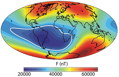
Figure 1. Intensity geomagnetic field map at 2015.0. The intensity values were generated by using the Gauss coefficients of the Swarm Level2 product (MCO—L2 DCO Core field model).

The region over the SAA (see Figure 1) is characterized by a high radiation close to the Earth's surface due to the very weak local geomagnetic field and, consequently, it represents the favorite entrance of high-energy particles in the magnetosphere, together with the polar regions (Vernov et al., 1967; Heirtzler, 2002). This effect is not only problematic at high altitude, where the satellites or other objects orbiting around the Earth are affected by a high density of cosmic ray particles, but also at surface level, where the communications can be disturbed due to the induced currents in transmission lines during geomagnetic storms (Trivedi et al., 2005). As an example, the International Space Station does require extra shielding to deal with this problem (McFee, 1999) and the Hubble Space Telescope interrupts data acquisition while passing through the SAA. Moreover, astronaut health is also affected by the augmented radiation in this region that is thought to be responsible for the peculiar “shooting stars” happening in their visual field (Casolino, 2003).

Thanks to the present high resolution geomagnetic models we know the inner origin of the SAA. The SAA at the Earth's surface is the response of an inverse flux path at the core-mantle boundary (CMB) of the radial component of the geomagnetic field located approximately under the South Atlantic Ocean generating the hemisphere asymmetry of the geomagnetic field (e.g., Heirtzler, 2002). The SAA behavior seems to indicate that this asymmetry could be connected to the general decrease of the dipolar field and to the significant increase of the non-dipolar field in the Southern Atlantic region (e.g., Gubbins et al., 2006; Aubert, 2015; Finlay et al., 2016, among others).

Since the geomagnetic field changes on space and time and its magnetic dipole strength is continuously decreasing (Thébault et al., 2015), the future of this large anomaly is a challenge of theoretical and practical importance due to the high influence effects on human health and the impact on instrumental efficiency. In fact, the decreasing of the intensity values of the SAA is far from a regional effect, and the depressed values of the SAA cover a large area in the South Atlantic Ocean and adjacent areas (Figure 1). In addition, very recent studies (De Santis et al., 2013) indicate that the area extent of the SAA follows a log-periodic acceleration that resembles the behavior of a critical system moving toward a critical transition. This behavior of the geomagnetic field seems present since there are available historical or instrumental measurements of the geomagnetic field. Another interesting feature is that this low value of the geomagnetic field strength at low latitudes is complemented by an increase in the polar regions (as the case of the so-called Siberia High) and this is the classical scenario for a geomagnetic field excursion or reversal.

The main goal of this paper is to analyse in details the evolution of the SAA not only at the Earth's surface but also at the CMB using the most recent data and models, to provide some clues about a possible impending excursion or reversal of the geomagnetic field. We first analyse the past evolution of the SAA at the Earth's surface during the last ~200 years (1840–2015) using two different geomagnetic field models (Section The SAA During the Last 200 years). Then, the Section The Origin of the SAA: A Case Study for the Last 200 years contains a detailed study about its origin at the CMB and finally, the connection to a possible upcoming transition of the Earth's magnetic field is discussed along with the main results in the Section Discussion.

The SAA During the Last 200 Years

In order to have a better understanding about the current behavior of the SAA we have carried out a study of the spatial and temporal evolution of this geomagnetic feature for the last two centuries.

For the oldest period, we use the historical geomagnetic model GUFM1 (Jackson et al., 2000). This global model was developed by using the Spherical Harmonic (SH) functions in space up to degree 14 and cubic splines in time, covering the period from 1590 to 1990. Jackson et al. (2000) solved the lack of intensity information before 1832 assuming a linear extrapolation of the first Gauss coefficient ${\text{g}}_1^0$ before 1840 according to its evolution during the most recent epochs, i.e., 1840–1990. This coefficient is an important key to study the behavior of the SAA since the intensity element strongly depends on it. In other words, the intensities of the GUFM1 model are not well constrained before ~1840 and this must be taken into account when the SAA area extent is calculated. In fact, if we calculate the SAA area extent following the new versions provided by Gubbins et al. (2006) and Finlay (2008) a clear difference is found before 1840 (see Figure 2) among the different models. These latter authors developed the new models using all the available intensity paleomagnetic data (Korte et al., 2005) from 1590 to 1840 following different approaches and provided a new value for the first Gauss coefficient for this period. However, no definitive answer can be given presently about which model is the best. For this reason, we prefer to start our study after 1840 where the ${\text{g}}_1^0$ coefficient is well-constrained by historical/instrumental intensity data.

FIGURE 2

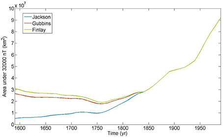
Figure 2. SAA extent area according to different historical global models (see legend).

From 1900 to 2015, we use the last generation of the International Geomagnetic Reference Field, i.e., the IGRF-12 (Thébault et al., 2015). This model, proposed every 5 years by the International Association of Geomagnetism and Aeronomy (IAGA), provides a global description of the geomagnetic main field up to harmonic degree of 13 using data from satellites and from observatories and surveys around the world. The IGRF-12 also contains the new high-quality satellite data from the Swarm mission since November 2013.

The use of global models to analyse the behavior of the SAA is not innovative and some studies have been already carried out using the GUFM1 model, such as the work of Hartmann and Pacca (2009). They applied the GUFM1 model along with observatory data from four geomagnetic observatories located in South America (Argentina and Brazil). The results show that the SAA at the Earth's surface is characterized by a west-southward drift with variable rates for the last 400 years. They defined the SAA region by the intensity isoline of 28,000 nT and according to that, the intensity within this region is decreasing as also corroborated by the observatory data. Finally, these authors analyzed at the Earth's surface the non-dipolar contribution of the GUFM1 model indicating that the SAA is governed by the quadrupolar and octupolar terms. A more recent study (De Santis and Qamili, 2010) modeled the SAA as the superposition of the axial geomagnetic field and a local equivalent monopolar sourced at the proximity of the CMB by using the GUFM1 model predictions. Using this approximation they characterized the SAA by an “equivalent monopole” which is moving close to the CMB with a mean drift of 10–20 km/year in an anticyclonic rotation centered at 55°S latitude and 0°E longitude. De Santis et al. (2013) defined the SAA at the Earth's surface as the region limited by the intensity isoline of 32,000 nT and they calculated the area extent using the GUFM1 model. Results from that work indicate that the area extent of the SAA has been continuously growing since there are available historical or instrumental geomagnetic data (see Figure 2).

In this study, we revisit the use of the model GUFM1 and, for the first time, we use the IGRF-12, both to analyse different characteristics of the SAA during the last 200 years:

(a) Minimum intensity of the SAA at the Earth's surface. In order to locate the position and the value of the minimum intensity inside the SAA region, we have performed an iterative approach based on the intensity gradient field using both global models in steps of 5 year from 1840 to 2015. Figures 3A, B show the movement and the value of the intensity minimum, respectively. The minimum intensity curve is characterized by a continuous decrease with a mean SV of −30 nT/year. On the other hand, as indicated by Hartmann and Pacca (2009), the movement of the SAA is directly linked with the westward drift of the geomagnetic field due to the non-dipolar field evolution. In fact, the velocity of the intensity minimum for the last decades agrees pretty well with the rate of the present westward drift, i.e., ~0.18°/year (Dumberry and Finlay, 2007).

(b) SAA area extent at the Earth's surface. We have calculated the area extent of the SAA using both models. The area has been calculated by interpolation in a regular grid over the Earth's surface with 4 × 10⁴ points. The SAA region was delimited by the intensity contour line of 32,000 nT. Our results (see Figure 4A) agree with those of De Santis et al. (2013) showing how the SAA area extent has been continuously growing. However, our results reveal more details (see Figure 4B): the SAA area extent is increasing with periods of accelerations (1840–1875 and 1900–1960) and decelerations (1975–1900 and 1960–2015). To complement this study, an animation showing the evolution of the SAA (every 5 years) in terms of intensity maps is given as Supplementary Material (Figure S1).

FIGURE 3

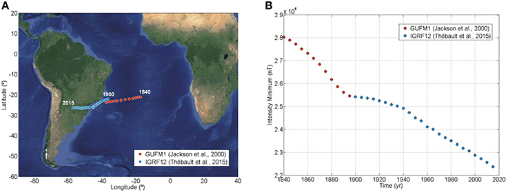
Figure 3. Location (A) and values (B) of the minimum intensity from 1840 to 2015 given by the GUFM1 (red points) and the IGRF-12 (blue points) models.

FIGURE 4

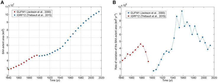
Figure 4. SAA extent area (A) and its first time derivative (B) given by the GUFM1 (red points) and IGRF-12 (blue points) models.

The Origin of the SAA: a Case Study for the Last 200 Years

According to Gubbins et al. (2006) the present decay of the dipole geomagnetic field is related to the extent area of the SAA. However, this effect must be considered at global scale because the dipole field, which is defined by the harmonic degree n = 1, takes into account the largest spatial wavelengths. In other words, the decay of the dipolar field increases the extent area of the SAA and decreases the averaged total intensity field at global scale. On the other hand, according to other studies (Hartmann and Pacca, 2009; De Santis et al., 2013), the behavior of the SAA during the last centuries is related to the higher harmonic degrees n = 2 and 3, i.e., the quadrupole and octupole fields. This is an important issue because these non-dipolar contributions play an important role during the geomagnetic reversals that are characterized by high ratios between the non-dipolar over dipolar contribution (e.g., Valet et al., 1999).

In this paper we have analyzed in more details how these both contributions, i.e., the dipolar (n = 1) and non-dipolar (n > 1), affect to the evolution of the SAA during the last two centuries. To do that, we first study the origin of the SAA using the radial component of the geomagnetic field provided by the GUM1 and IGRF-12 models. The Figure 5 shows different maps of this geomagnetic element at the CMB for four separated epochs from 1840 to 2015. As expected, when the dipolar field is only considered (maps A, B, C, D) the element B_r presents a clear symmetry at the CMB with positive/negative values in the Southern/Northern geomagnetic Hemisphere. However, the addition of the quadrupole (n = 2) to the previous one breaks this symmetry just under the South Atlantic Ocean showing a clear anomaly in this area at the CMB (maps E, F, G, H). Finally, when one includes the octupole (n = 3) the symmetry totally disappears (maps I, J, K, L) and a region of reversal flux polarity appears and expands in time under the South Atlantic Ocean becoming a clear and isolated reversal flux polarity at 2015 (Map L). To complement these maps, we have also plotted the intensity maps at the Earth's surface to highlight the effect in the SAA using the same harmonic contributions and epochs (see Figure S2 of the Supplementary Material). As shown by the different maps, the dipole affects the intensity values at global scale showing low values in the most recent times (decay of the dipolar field, maps A, B, C, D in Figure S2). On the contrary, the quadrupolar and octupolar fields create a clear reversal path at the CMB that generates the low intensity values at the Earth's surface centered over the Southern Atlantic Ocean and adjacent areas.

FIGURE 5

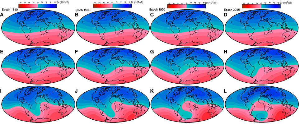
Figure 5. Maps of the radial element of the geomagnetic field, Br, at the CMB for different epochs and different harmonic contributions (values given by the GUFM1 and IGRF-12 geomagnetic global models). (A–D) Dipole field; (E–H) Dipole + Quadrupole field; and (I–L) Dipole + Quadrupole + Octupole field.

The next step is to calculate the SAA extent area using the different harmonic contributions. The procedure to calculate the SAA extent area is that detailed in the previous Section SAA Area Extent at the Earth's Surface. The difference lies in the values of the Gauss coefficients involved in the first three harmonic degrees. We have kept constant the value of the Gauss coefficient at the beginning of the temporal windows, i.e., at 1840. Figure 6 shows the results of the different SAA extent areas according to the different constant harmonic contributions. The black line is the original SAA extent area when any Gauss coefficient is modified (equal to that of the Figure 4A). The quantitative effect on the SAA extent area due to a constant dipole (red line) or quadrupole (blue line) is approximately the same with a reduction of the area around 50% smaller than the original one for the total temporal window. This percentage increases up to 85% when we consider both contributions together (yellow line). Finally, a constant octupolar contribution does not significantly affect the extent area (green line), but when this is added to the previous constant dipole and quadrupole, the SAA extent area does not present important changes during the last 200 years (violet line).

FIGURE 6

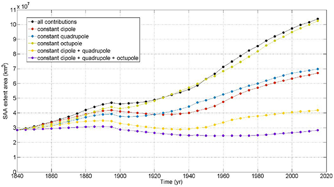
Figure 6. SAA extent area keeping constant some harmonic contributions at 1840, i.e., the initial epoch of the instrumental intensity measurement. The extent area is provided by the intensity isoline of 32,000 nT at the Earth's surface by the GUFM1 and IGRF-12 models.

Discussion

The last complete reversal of the Earth's magnetic field occurred 780.000 years ago: the Matuyama–Bruhnes (M–B) polarity reversal, where the north magnetic pole moved toward the Southern geographic pole reaching the present normal polarity. This feature has been deeply studied becoming the best documented past geomagnetic event in the basis of the huge density of paleomagnetic data recording this polarity transition (see Valet et al., 1999 for a review). During the last decade, these paleomagnetic data have been used to model the behavior of the geomagnetic field during this transition (Leonhardt and Fabian, 2007) or to constrain the geodynamo numerical simulations (e.g., Aubert et al., 2008) pointing out different scenarios for the precedent phase of a geomagnetic reversal.

One of the most accepted hypothesis is that the geomagnetic transitions are preceded by the apparition of flux patches of reversed polarity at low or mid latitude that then migrate poleward reducing the axial dipolar field (Aubert et al., 2008; Wicht and Christensen, 2010; among others). In fact, during a reversal the dipolar strength (geomagnetic dipolar moment, DM) decays up to values around 10–20% lower than those characteristic for a geomagnetic chron (see the DM curves provide by Valet et al., 2005; or Channel et al., 2009). At the same time, the non-dipolar contributions take an important role as highlighted by the diversity on the virtual geomagnetic pole tracks found in paleomagnetic studies focused on the same geomagnetic event (see, for example, Laj et al., 2006 where the Laschamp geomagnetic excursion is analyzed).

According to the above-mentioned patterns, one could think that the present geomagnetic field is going to a transition because: (a) an increasing of the non-dipolar contributions and a well-known decay of the dipole field characterize it; (b) two prominent patches of reversal polarity are located at the CMB in the south part of America and Africa; (c) simple statistical calculations show that the average time between reversals is 400 kyear and the last reversal occurred 780 kyear ago.

In order to analyse in more details at least the first two above patterns, we have used the GUFM1 and IGRF-12 geomagnetic models from 1840 to 2015.

Figure 7 contains the energy of the dipolar and the non-dipolar fields, in terms of the power spectra of the Gauss coefficients at the Earth's surface, for both models since the beginning of the instrumental measurements of the intensity element, i.e., 1840. Results show that the dipolar filed is decreasing with a rate of −12% per century and this rate is faster than expected for geomagnetic diffusion and agrees with the found decay rates in geomagnetic transitions (Laj and Kissel, 2015). In addition, the energy of the non-dipolar field is increasing in time with a pronounced rate of +70% per century.

FIGURE 7

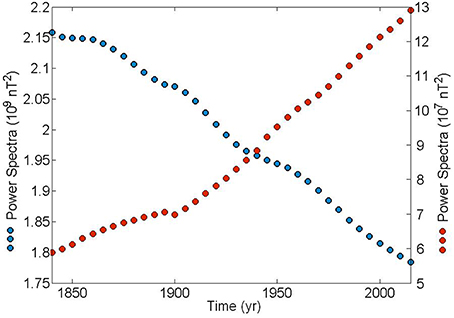
Figure 7. Energy, in term of the power spatial spectra, of the mean square value, of the dipole field (left vertical axis and blue dots) and non-dipole field (right vertical axis and red dots) at the Earth's surface for the last 200 years according to the models GUFM1 and IGRF-12. The non-dipole field is given by the harmonic contributions from 2 to 6.

However, the previous scenario seems to be far from those that characterize a geomagnetic transition, because the present value of the DM seems to be not anomalous if we compare it with the DM during the Holocene (last 12 ka) and the complete Brunhes polarity chron (last 0.78 ka). For the first case, i.e., the Holocene, we have used the global model SHA.DIF.14k (Pavón-Carrasco et al., 2014). As indicated in the Figure 8A, during the Holocene the DM oscillates between 4 and 11 × 10²²A·m² with a mean value equal to 8.1 ± 1.6 × 10²²A·m². For older times, we used the SINT800 (Guyodo and Valet, 1999) and the PISO-1500 (Channel et al., 2009) curves that provide the DM (in this case is the virtual axial dipole moment) for the last 800 ka and 1.5 Ma, respectively. Both curves show the values of the DM during geomagnetic transitions: 7 excursions (pink arrows in Figure 8B) and the B–M reversal (green arrow in Figure 8B). As shown, the values of the DM for these events are low with values around 3 × 10²²A·m² for the excursion and lower than 1 × 10²²A·m² for the B-M reversal. The average DM for the entire chron is 6.0 ± 1.5 × 10²² and 7.1 ± 2.7 × 10²² A·m² considering SIN800 and PISO-1500, respectively.

FIGURE 8

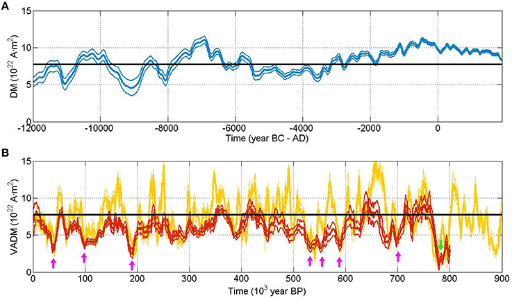
Figure 8. (A) Dipolar moment and error at 2σ (blue curve) according to the SHA.DIF.14k model for the last 12 ka. (B) Virtual axial dipole moment given by the SINT800 (red curve with error at 1σ) and PISO-1500 (yellow curve with error at 1σ) paleomagnetic curves for the last 900 ka. Pink arrows correspond to geomagnetic excursions and the green arrow to the B–M transition. The black horizontal lines show the value of the dipolar moment at 2015.0 given by the Level2 product of Swarm.

The comparison with the present value of the DM (7.7 10²² A·m², provided by the Swarm Level2 products at 2015.0) shows that even if the dipole field is decaying during the last centuries, the value of the DM agrees with the mean value of the DM during the Holocene and is higher than the typical values of DM during excursions (~3 × 10²² A·m²) and the B-M reversal (lower than 1 × 10²² A·m²).

In terms of reversal polarity patches at the CMB, we have analyzed the radial component at the CMB (only up to harmonic degree 6) using the geomagnetic models from 1840 to 2015 (see Figure 9). At the beginning of our temporal windows, there is only a reversal polarity patch at the CMB covering the major part of the South Atlantic Ocean (Figure 9A). This patch moved westward, growing in extension and then around 1900 split up in two different patches (Figures 9B–D; see the series of maps every 5 year in the Figure S3 of the Supplementary Material). From this time, the extent area of the reversal flux patch located in the south America (with center which is close to the Falkland islands) remains constant during the last 115 years, however the other patch located in the Atlantic ocean between Africa and Antarctica becomes more accentuated and with a clear western drift. However, we want to warn that this behavior before 1900 (i.e., one reversal patch) could not be real due to the lower resolution of the GUFM1 model in comparison with the IGRF-12 model. This study is complemented by the behavior of the minimum values of the geomagnetic radial element B_r for both reversal patches (see Figure 9E). The minimum value of B_r for the African patch is decreasing with a rate of −2.54·10⁵ nT per century causing the growth of the area of this patch at the CMB. On the contrary, the American patch seems to be vanishing since the minimum value of B_r presents a positive rate of change: +0.67·10⁵ nT per century.

FIGURE 9

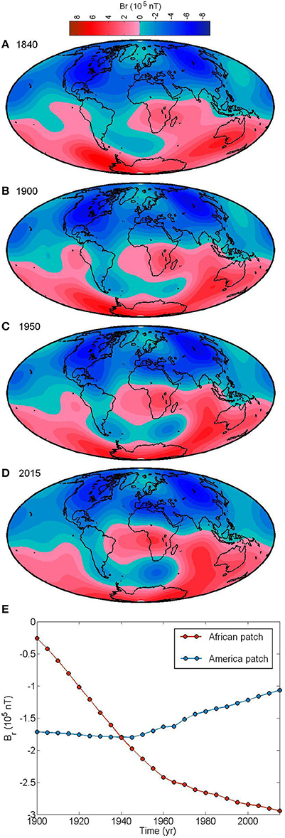
Figure 9. Radial element Br of the geomagnetic field at the CMB at (A) 1840, (B) 1900, (C) 1950, and (D) 2015. (E) Temporal evolution of the minimum of the radial field at the CMB for each reversal patch from 1900 to 2015.

The found patches seems to be in agreement with the hypothesis recently revisited by Tarduno et al. (2015) where the authors suggest that the appearance of these patches of reversal polarity are linked with the boundaries of the African large low shear velocity province (LLSVP). The LLSVP is an abrupt area at the CMB under South Africa characterized by a low seismic wave anomaly. Tarduno et al. (2015) propose that the core flow in areas close to the African LLSVP develops upward component at small scales allowing reversed polarity flux bundles to leak upward, but they also admit that more detailed theoretical and numerical simulations are needed to confirm their hypothesis.

Finally, in terms of statistics, the average occurrence of geomagnetic transition for the last 83 Ma is 400 kyear (De Santis et al., 2013). They calculated the average value only for the last 83 Ma to avoid the Cretaceous Normal Superchron (from 83 to 121 Ma) where the geomagnetic field kept the same normal polarity for 38 Myear. If we take into account that the last reversal occurred 780 ka, this simple statistical study suggests that the geomagnetic field is taking a very long time to reach a new reversal, higher than the mean value of 400 kyear. However, we also point out that Constable and Korte (2006) have shown that the probability of observing a chron as long as the present Brunhes chron is not improbable.

To come back to the three features for having a reversal, i.e., (a) decay dipole field, (b) reversal patches at the CMB in middle latitudes, and (c) a mean rate of 400 kyear for reversals, we can conclude that the patterns (b) and (c) agree with an upcoming transition of the Earth's magnetic field. Nevertheless, the first one (a) is not clear: although the dipole field decays faster than expected for geomagnetic diffusion, the present value of the DM is not comparable with those given by the geomagnetic transitions recorded in rocks. However, it is interesting to note that the present rate of decay is comparable with that occurred during previous reversals (Laj and Kissel, 2015).

Conclusions

In this work we have analyzed in details the cons and pros of a possible upcoming geomagnetic transition, paying special attention to the continuous increase of the SAA extent area. Our results carried out during the last 200 year, reveals that the geomagnetic field presents two patches of reversal polarity at the CMB that are growing and moving toward west. Both patches are characterized by negative values of the radial component of the geomagnetic field and the African patch is growing with a rate of −2.54·10⁵ nT per century. In addition, we have demonstrated that the quadrupole field mainly controls these reversal patches at the CMB and this agrees with the previous phase of a geomagnetic transition. However, the obtained DM is not so low when compared with recent paleomagnetic data for the Holocene and with the mean DM value for the entire Brunhes geomagnetic polarity (last ~0.8 Ma), and this is an important key in the preparation phase of an imminent geomagnetic transition. The new Swarm mission is providing more new and high-quality geomagnetic data that can shed light on this challenge, because the continuous monitoring of the recent SAA is fundamental to understand the next directions of the geomagnetic field.

Author Contributions

FP established the original idea, carried out the calculations, and wrote the manuscript with the contribution of AD.

Conflict of Interest Statement

The authors declare that the research was conducted in the absence of any commercial or financial relationships that could be construed as a potential conflict of interest.

Acknowledgments

FP and AD thank L.M. Alva and C. Laj for their comments on this manuscript. FP is grateful to the ESA-funded Project TEMPO (contract N° 4000112784/14/I-SBo, The Living Planet Fellowship) and to the postdoctoral Marie Skłodowska-Curie Individual Fellowship 659901-CLIMAGNET. AD thanks the ESA-funded Project SAFE (contract n° 4000113862/15/NL/MP-Swarm+Innovation) and the INGV-funded LAIC-U Project, for providing financial support to this research. All algorithms have been developed in Matlab codec (Matlab 7.11.0, R2010b) along with the figures. The models and data used are listed in the references, tables and in the main manuscript.

Supplementary Material

The Supplementary Material for this article can be found online at: https://www.frontiersin.org/article/10.3389/feart.2016.00040

References

Aubert, J. (2015). Geomagnetic forecasts driven by thermal wind dynamics in Earth's core. Geophys. J. Int. 203, 1738–1751. doi: 10.1093/gji/ggv394

CrossRef Full Text | Google Scholar

Aubert, J., Aurnou, J., and Wicht, J. (2008). The magnetic structure of convection-driven numerical dynamos. Geophys. J. Int. 172, 945–956. doi: 10.1111/j.1365-246X.2007.03693.x

CrossRef Full Text | Google Scholar

Casolino, M., Bidoli, V., Morselli, A., Narici, L., De Pascale, M. P., Picozza, P., et al. (2003). Space travel: Dual origins of light flashes seen in space. Nature 422, 680. doi: 10.1038/422680a

CrossRef Full Text | Google Scholar

Channel, J. E. T., Xuan, C., and Hodell, D. A. (2009). Stacking paleointensity and oxygen isotope data for the last 1.5 Myr (PISO-1500). Earth Planet. Sci. Lett. 283, 14–23. doi: 10.1016/j.epsl.2009.03.012

CrossRef Full Text | Google Scholar

Constable, C., and Korte, M. (2006). Is the Earth's magnetic field reversing? Earth Planet. Sci. Lett. 246, 1–16. doi: 10.1016/j.epsl.2006.03.038

CrossRef Full Text | Google Scholar

De Santis, A., and Qamili, E. (2010). Equivalent monopole source of the geomagnetic South Atlantic Anomaly. Pure Appl. Geophys. 167, 339–347. doi: 10.1007/s00024-009-0020-5

CrossRef Full Text | Google Scholar

De Santis, A., Qamili, E., and Wu, L. (2013). Toward a possible next geomagnetic transition? Nat. Hazards Earth Syst. Sci. 13, 3395–3403. doi: 10.5194/nhess-13-3395-2013

CrossRef Full Text | Google Scholar

Dumberry, M., and Finlay, C. C. (2007). Eastward and westward drift of the Earth's magnetic field for the last three millennia. Earth Planet. Sci. Lett. 254, 146–157. doi: 10.1016/j.epsl.2006.11.026

CrossRef Full Text | Google Scholar

Finlay, C. C. (2008). Historical variation of the geomagnetic axial dipole. Phys. Earth Planet. Int. 170, 1–14. doi: 10.1016/j.pepi.2008.06.029

CrossRef Full Text | Google Scholar

Finlay, C. C., Aubert, J., and Gillet, N. (2016). Gyre-driven decay of the Earth's magnetic dipole. Nat. Commun. 7:10422. doi: 10.1038/ncomms10422

CrossRef Full Text | Google Scholar

Finlay, C. C., Olsen, N., and Tøffner-Clausen, L. (2015). DTU candidate field models for IGRF-12 and the CHAOS-5 geomagnetic field model. Earth Planets Space 67, 114. doi: 10.1186/s40623-015-0274-3

CrossRef Full Text | Google Scholar

Gauss, C. F. (1833). Intensitas vis magneticae terrestris ad mensuram absolutam revocata. R. Sci. Soc. 8, 3–44.

Google Scholar

Gubbins, D., Jones, A. L., and Finlay, C. C. (2006). Fall in Earth's magnetic field is erratic. Science 312, 900–902. doi: 10.1126/science.1124855

PubMed Abstract | CrossRef Full Text | Google Scholar

Guyodo, Y., and Valet, J. P. (1999). Global changes in intensity of the Earth's magnetic field during the past 800 kyr. Nature 399, 249–252. doi: 10.1038/20420

CrossRef Full Text | Google Scholar

Hartmann, G. A., and Pacca, I. G. (2009). Time evolution of the South Atlantic Magnetic Anomaly. Ann. Braz. Acad. Sci. 81, 243–255. doi: 10.1590/S0001-37652009000200010

CrossRef Full Text | Google Scholar

Heirtzler, J. R. (2002). The future of the South Atlantic anomaly and implications for radiation damage in space. J. Atmos. Solar Terr. Phys. 64, 1701–1708. doi: 10.1016/s1364-6826(02)00120-7

CrossRef Full Text | Google Scholar

Jackson, A., Jonkers, A. R. T., and Walker, M. R. (2000). Four centuries of geomagnetic secular variation from historical records. Philos. Trans. R. Soc. Lond. A 358, 957–990. doi: 10.1098/rsta.2000.0569

CrossRef Full Text | Google Scholar

Jonkers, A. R. T., Jackson, A., and Murray, A. (2003). Four centuries of geomagnetic data from historical records. Rev. Geophys. 41, 1006. doi: 10.1029/2002rg000115

CrossRef Full Text | Google Scholar

Korte, M., Genevey, A., Constable, C. G., Frank, U., and Schnepp, E. (2005). Continuous geomagnetic field models for the past 7 millennia: 1. A new global data compilation. Geochem. Geophys. Geosyst. 6, Q02H15. doi: 10.1029/2004gc000800

CrossRef Full Text | Google Scholar

Laj, C., and Kissel, C. (2015). An impending geomagnetic transition? Hints from the past. Front. Earth Sci. 3:61. doi: 10.3389/feart.2015.00061

CrossRef Full Text | Google Scholar

Laj, C., Kissel, C., and Roberts, A. P. (2006). Geomagnetic field behavior during the Icelandic basin and Laschamp geomagnetic excursions: a simple transitional field geometry? Geochem. Geophys. Geosyst. 7, Q03004. doi: 10.1029/2005GC001122

CrossRef Full Text | Google Scholar

Leonhardt, R., and Fabian, K. (2007). Paleomagnetic reconstruction of the global geomagnetic field evolution during the Matuyama/Brunhes transition: iterative Bayesian inversion and independent verification, Earth Planet. Sci. Lett. 253, 172–195. doi: 10.1016/j.epsl.2006.10.025

CrossRef Full Text | Google Scholar

McFee, C. (1999). Radiation Shielding Considerations for the Solar-B EIS CCDs – Initial Discussion. EIS-CCD-desnote-003 in Solar-B, EIS. EUV Imaging Spectrometer.

Olsen, N., and Haagmans, R. (eds.). (2006). Swarm—the earth's magnetic field and environment explorers. Earth Planets Space 58, 349–496. doi: 10.1186/BF03351932

CrossRef Full Text | Google Scholar

Pavón-Carrasco, F. J., Osete, M. L., Torta, J. M., and De Santis, A. (2014). A geomagnetic field model for the Holocene based on archaeomagnetic and lava flow data. Earth Planet. Sci. Lett. 388, 98–109. doi: 10.1016/j.epsl.2013.11.046

CrossRef Full Text | Google Scholar

Sabaka, T. J., Olsen, N., Tyler, R. H., and Kuvshinov, A. (2015). CM5, a pre-Swarm comprehensive geomagnetic field model derived from over 12 yr of CHAMP, Ørsted, SAC-C and observatory data. Geophys. J. Int. 200, 1596–1626. doi: 10.1093/gji/ggu493

CrossRef Full Text | Google Scholar

Tarduno, J. A., Watkeys, M. K., Huffman, T. N., Cottrell, R. D., Blackman, E. G., Wendt, A., et al. (2015). Antiquity of the South Atlantic Anomaly and evidence for top-down control on the geodynamo. Nat. Commun. 6, 7865. doi: 10.1038/ncomms8865

PubMed Abstract | CrossRef Full Text | Google Scholar

Thébault, E., Finlay, C. C., Beggan, C. D., Alken, P., Aubert, J., Barrois, O., et al. (2015). International Geomagnetic Reference Field: the 12th generation. Earth Planets Space 67, 79. doi: 10.1186/s40623-015-0228-9

CrossRef Full Text | Google Scholar

Trivedi, N. B., Pathan, B. M., Schuch, N. J., Barreto, L. M., and Dutra, L. G. (2005). Geomagnetic phenomena in the South Atlantic Anomaly region in Brazil. Adv. Space Res. 36, 2021–2024. doi: 10.1016/j.asr.2004.09.020

CrossRef Full Text | Google Scholar

Valet, J.-P., Brassart, J., Quidelleur, X., Soler, V., Gillot, P. Y., and Hongre, L. (1999). Paleointensity variations across the last geomagnetic reversal at La Palma, Canary Islands, Spain. J. Geophys. Res. 104, 7577–7598. doi: 10.1029/1998JB900099

CrossRef Full Text | Google Scholar

Valet, J.-P., Meynadier, L., and Guyodo, Y. (2005). Geomagnetic dipole strength and reversal rate over the past two million years. Nature 435, 802–805. doi: 10.1038/nature03674

PubMed Abstract | CrossRef Full Text | Google Scholar

Vernov, S. N., Gorchakov, E. V., Shavrin, P. I., and Sharvina, K. N. (1967). Terrestrial corpuscular radiation and cosmic rays. Space Sci. Rev. 7, 490–533.

Google Scholar

Wicht, J., and Christensen, U. R. (2010). Torsional oscillations in dynamo simulations. Geophys. J. Int. 181, 1367–1380. doi: 10.1111/j.1365-246x.2010.04581.x

CrossRef Full Text | Google Scholar