Energetics of Slope Flows: Linear and Weakly Nonlinear Solutions of the Extended Prandtl Model

Introduction

Katabatic and anabatic winds are downslope and upslope flows that form when a density difference between the air near the slope and the nearby atmosphere develops at the same height. This type of flow is often observed in regions of complex orography and substantially affects the weather and climate in these regions (e.g., Poulos and Zhong, 2008). The topic of katabatic and anabatic wind is being actively explored and the work on its understanding includes the application of numerical models (direct numerical simulations (DNS): (e.g., Shapiro and Fedorovich, 2008); large eddy simulations (LES): e.g., Skyllingstad, 2003; Smith and Porté-Agel, 2013); mesoscale models: (e.g., Smith and Skyllingstad, 2005; Zammett and Fowler, 2007); and analytical models (e.g., Prandtl, 1942; Defant, 1949; Grisogono and Oerlemans, 2001; Zardi and Serafin, 2014). Continued interest in katabatic and anabatic winds stems from the important effects of this type of orographic flows on visibility and fog formation, air pollutant dispersion, agriculture and energy use, fire-fighting operations, sea-ice formation, etc. (e.g., Shapiro and Fedorovich, 2014, and references therein). Katabatic winds develop in stably stratified planetary boundary layers (PBLs), adding an additional level of complexity to the problem of understanding and modeling this specific type of PBLs (e.g., Mahrt, 1998; Holtslag et al., 2013; Sandu et al., 2013; Mahrt, 2014; Sun et al., 2015). In reality, a strong surface heat surplus may contribute to a high Rayleigh number and initiation of free convection over the horizontal plane (e.g., Princevac and Fernando, 2007). This condition may limit the general applicability of the Prandtl model and its extensions to the case of anabatic flow for a large surface temperature surplus. However, Defant (1949) and Fedorovich and Shapiro (2009a,b) as well as several other authors, show clearly that the Prandtl model is applicable, at least qualitatively, to anabatic flow. Although the latter authors state that turbulent anabatic flows differ more, in a mean qualitative sense, from its Prandtl model version for katabatic flows, they still show and claim the overall applicability of the Prandtl model (at least qualitatively) to both flow types. In parallel to current theoretical and numerical modeling efforts, large observational campaigns and programs over complex orography should be of a high priority in order to better understand the nature of thermally driven slope flows (e.g., Poulos and Zhong, 2008; Fernando et al., 2015; Grachev et al., 2015).

In the model of Prandtl (1942), katabatic flow is the result of a balance between the along-slope buoyancy force and adiabatic warming/cooling, and normal-to-slope turbulent fluxes of momentum (i.e., friction) and heat (i.e., diffusion), respectively, in an otherwise motionless and statically stable background atmosphere. This paper starts with the classical theoretical model of slope flows developed by Prandtl (1942), somewhat modified and verified by Defant (1949), who deployed it specifically for anabatic flow (see also Zardi and Whiteman, 2013), and an extended Prandtl model that includes weakly nonlinear effects as done in Grisogono et al. (2015). It includes the standard concepts of potential, kinetic and total energy, now for katabatic and anabatic flows. In the energetics framework, wind speed and temperature perturbations are linked in one equation (i.e., the total energy equation) and the conservation and conversion properties of energy components are of special concern in various research problems (e.g., the effect of turbulent mixing may be parameterized in terms of kinetic energy). The energy approach applied here is motivated by the total turbulent energy concept developed by e.g., Mauritsen et al. (2007), where kinetic energy is related to turbulent wind perturbations, while potential energy is related to turbulent potential temperature perturbations. In our case, we focus only on mean katabatic and anabatic flows that are present over sloped surfaces. The difference, when compared to Mauritsen et al. (2007), is in our focus not being on the turbulent part of the flow but on the wind and temperature finite amplitude deviations from the background state coming from katabatic/anabatic flows. In this sense, our approach is similar to the energy framework of katabatic winds applied by Smith and Skyllingstad (2005). While, Smith and Skyllingstad (2005) define kinetic energy in the same way as Mauritsen et al. (2007), their potential energy is defined as a linear function of both temperature perturbations and the height above the slope. Although there are some differences in the literature concerning the definition of potential energy, it is typically a function of potential temperature perturbations. Potential temperature perturbations, under the assumptions of hydrostatic and adiabatic motion, include the effects of absolute temperature perturbations and changes in the distance from the surface (e.g., DeCaria, 2007). The total energy is then the sum of kinetic and potential contributions.

We limit ourselves only to the linear and weakly nonlinear solution of the (extended) Prandtl model. A detailed description of the extended Prandtl model is presented in Grisogono et al. (2015; their Section 2). The new term that extends the original Prandtl model is presumably weak and regulated by the nonlinearity parameter ε. Our approach is relatively simple and general, and may be applied to solutions of Prandtl-type models that include 3D effects (e.g., Burkholder et al., 2009; Shapiro et al., 2012), effects of the Coriolis force (e.g., Stiperski et al., 2007), time-dependent types of solutions (e.g., Zardi and Serafin, 2014), effects of vertically varying turbulent mixing coefficients (e.g., Grisogono and Oerlemans, 2001; Grisogono et al., 2015), etc. To sum up, this study combines the work of Mauritsen et al. (2007) and Grisogono et al. (2015), i.e., the energy concept and weak nonlinearity, respectively, to shed more light on the physics of simple slope flows.

This study is independent but based on the work of Grisogono et al. (2015). There it was shown that with the weakly nonlinear Prandtl model one obtains solutions with stronger near-surface stratification and weaker katabatic wind speed (with both constant and variable eddy heat conductivity). However, although more realistic, the solutions of the weakly nonlinear model were not superior to the linear solutions when compared to limited observations. The nonlinearity affected low-level jet strength and elevation in katabatic, but also anabatic, flows. In anabatic flow, in contrast to katabatic flow, it enhanced the low-level jet. The consequences of the introduced nonlinearity on the model energetics will be explored in this paper.

The goal of this study is to evaluate an ensemble of linear and weakly nonlinear solutions of the (extended) Prandtl model for katabatic and anabatic flows, and to examine the model energetics related to these solutions. In order to explore the sensitivity of our results to several model assumptions, we present a set of solutions where three governing parameters are perturbed: (1) the turbulent Prandtl number Pr, (2) the slope angle α, and (3) the so-called nonlinearity parameter ε as defined in Grisogono et al. (2015). We will present certain characteristics of the solutions of the Prandtl model, the vertical profiles of kinetic KE, potential PE and total energy TE, and the governing terms in the total energy TE equation.

The structure of the paper is as follows. In Section Methodology, we present the governing equations of our model and define the ensemble of solutions. In Section Results, the solutions of the (extended) Prandtl model are described, with a specific focus on the variability in the ensemble of solutions and impacts on the model energetics. Some specific differences between the nonlinear and linear solutions, as well as the limitations of our extended Prandtl model are discussed in Section Discussion. The paper is finalized in Section Summary and Conclusions, where the summary and outlook are presented.

Methodology

We first present the governing equations of the Prandtl model and develop a simple, basic energy framework where wind and potential temperature are linked with the concepts of kinetic, potential and total energy. The full description of the system would include the energy components of not only the mean slope flow, but of the background atmosphere and the turbulent part of the slope flow, and their interactions. We limit our analysis only to the part of the slope flow described by the Prandtl model, i.e., the mean slope flow with relatively large eddy diffusivity and conductivity; hence, the model may emulate a simple turbulent slope flow (Defant, 1949; Stiperski et al., 2007; Grisogono et al., 2015).

Governing Equations

Potential temperature and wind can be decomposed into $\theta ={\theta }_r+\overline{\theta }+\theta \prime$ and $u=u_r+\overline{u}+u\prime$, where θ_r = θ₀ + γz is the potential temperature of the background atmosphere having the vertical gradient γ (in true vertical coordinate Z), and θ₀ is the surface potential temperature in a statically stable background atmosphere (e.g., Zardi and Serafin, 2014). The background atmosphere is motionless: u_r = 0. Next, u′ and θ′ are turbulent perturbations of the wind speed and potential temperature of the slope flow, while $\overline{u}$ and $\overline{\theta }$ represent the mean finite-amplitude wind speed and potential temperature (here, averaging is defined in the Reynolds sense).

The governing equations of the Prandtl model, including the weak nonlinearity extension (without invoking the steady-state assumption for the moment) are:

$\begin{array}{ll}\frac{\partial \overline{u}}{\partial t}=g\frac{\overline{\theta }}{{\theta }_0}sin\left(\alpha \right)+KPr\frac{{\partial }^2\overline{u}}{\partial z^2}& (1)\end{array}$

$\begin{array}{ll}\frac{\partial \overline{\theta }}{\partial t}=-\left(\gamma +\epsilon \frac{\partial \overline{\theta }}{\partial z}\right)\overline{u}sin\left(\alpha \right)+K\frac{{\partial }^2\overline{\theta }}{\partial z^2}& (2)\end{array}$

where g is acceleration due to gravity, K is the eddy heat conductivity, Pr is the turbulent Prandtl number (all assumed constant in this study), and z is the coordinate perpendicular to the constant slope surface with the slope angle α. Parameter ε controls the feedback of the flow-induced potential temperature gradient on to the corresponding background gradient, γ, because the former, below the low-level jet, can be 20–50 times stronger (in the absolute sense) than the latter (e.g., Grisogono and Oerlemans, 2001; Grisogono et al., 2015). ε is an external parameter, roughly limited by the model input parameters, not by the model dynamics, and it pertains to the regular perturbation analysis used here [(Bender and Orszag, 1978; Grisogono et al., 2015); see also Supplementary Materials 1 in this study]. After multiplying Equation (1) by $\overline{u}$, multiplying Equation (2) by $\overline{\theta }g∕\left({\theta }_0\gamma \right)$ or $\overline{\theta }a$, and adding the resulting two equations, the energy equation of the extended Prandtl model is attained:

$\begin{array}{l}\frac{\partial }{\partial t}\left(\frac{{\overline{u}}^2+a{\overline{\theta }}^2}{2}\right)=\\ {\displaystyle \underset{DIF}{{\displaystyle \underbrace{K\frac{{\partial }^2}{\partial z^2}\left(\frac{Pr{\overline{u}}^2+a{\overline{\theta }}^2}{2}\right)}}}}-{\displaystyle \underset{DIS}{{\displaystyle \underbrace{K\left[Pr{\left(\frac{\partial \overline{u}}{\partial z}\right)}^2+a{\left(\frac{\partial \overline{\theta }}{\partial z}\right)}^2\right]}}}}\\ -{\displaystyle \underset{INT}{{\displaystyle \underbrace{a\epsilon sin\left(\alpha \right)\left(\overline{u}\overline{\theta }\frac{\partial \overline{\theta }}{\partial z}\right)}}}}& (3)\end{array}$

where the left side term is the local storage term of TE of the mean slope flow defined as the sum of kinetic KE = $\overline{u^2}∕2$ and potential energy PE = $a{\overline{\theta }}^2$/2 per unit mass (cf. Smith and Skyllingstad, 2005; Mauritsen et al., 2007). The three terms on the right side are described as diffusion (DIF), dissipation (DIS), and interaction (INT) terms: DIF represents the diffusion of TE by the turbulent flow, DIS represents the dissipation of TE, and INT represents the interaction of the slope flow with the background atmosphere in the case of the weakly nonlinear model. Note that INT is equal to $\epsilon sin\left(\alpha \right)\left(\overline{u}\frac{\partial PE}{\partial z}\right)$, which can be interpreted as the slope-normal (i.e., nearly vertical) transport of potential energy. This term does not exist in the linear model.

Four types of steady-state solutions of Equations (1) and (2) are analyzed in Grisogono et al. (2015). They include linear and weakly nonlinear solutions with turbulent mixing coefficients either constant or vertically varying. In this paper, a subset of these solutions is analyzed (from now on, the overbar is removed from potential temperature $\overline{\theta }$ and wind speed $\overline{u}$ of katabatic/anabatic flow): (1) the linear solution with the constant turbulent diffusivity profile θ_LIN and u_LIN, and (2) the nonlinear solution with the constant turbulent diffusivity profile θ_NOLIN and u_NOLIN. Initial results concerning the vertical variability of K and its impact on energy distribution show sensitivity to the formulation of K(z) and strong non-stationarity even in the linear case; thus, a detailed analysis of this subset of solutions is left for future study. For simplicity, here we show only the classical solutions of the Prandtl model θ_LIN and u_LIN [for the nonlinear solutions please refer to Grisogono et al. (2015)]:

$\begin{array}{ll}{\theta }_{LIN}=Cexp\left(\frac{-z}{h_P}\right)cos\left(\frac{z}{h_P}\right)& (4)\end{array}$

$\begin{array}{ll}{u}_{LIN}=-\mu Cexp\left(\frac{-z}{h_P}\right)sin\left(\frac{z}{h_P}\right)& (5)\end{array}$

Following, e.g., Grisogono et al. (2015), C is the surface potential temperature deficit θ_LIN(z = 0) = C < 0 for the katabatic flow (or the corresponding temperature surplus in anabatic flow θ_LIN(z = 0) = C > 0), μ = [g/(γθ₀Pr)]^1/2, h_P = 2^1/2/σ (h_P can be interpreted as a characteristic depth of the Prandtl layer), σ = [N sin(α)/(KPr^1/2)]^1/2 (σ can be interpreted as a characteristic inverse length scale), N² = γg/θ_o is background buoyancy frequency squared, and K is the average eddy heat conductivity [in our case K = const in Equations (1) and (2)]. The slope flow is assumed to be no-slip (i.e., u_LIN(z = 0) = 0).

In the case of linear and stationary flow, Equation (3) simplifies to:

$\begin{array}{ll}0=\frac{{\partial }^2}{\partial z^2}\left(\frac{Pr{u}_{LIN}^2+a{\theta }_{LIN}^2}{2}\right)-\left[Pr{\left(\frac{\partial u_{LIN}}{\partial z}\right)}^2+a{\left(\frac{\partial {\theta }_{LIN}}{\partial z}\right)}^2\right]& (6)\end{array}$

and one can easily check the equality by inserting Equations (4) and (5) into Equation (6). In the rest of the paper, we determine vertical derivatives using finite differences in the case of both linear and weakly nonlinear types of solution.

Ensemble of Solutions

We evaluate the sensitivity of our solutions to the slope angle α, the value of the Prandtl number Pr and the nonlinearity parameter ε. Based on Grisogono et al. (2015), the basic values of these model parameters are α = −0.1 rad, Pr = 2 and ε = 0.005/0.03 (katabatic/anabatic flow) where the justification of these parameter choices is discussed in more detail by Grisogono et al. (2015). The starting values of all three parameters are taken from Grisogono et al. (2015), where linear and nonlinear solutions reproduced well the observations from the PASTEX-94 experiment (van den Broeke, 1997a,b; Oerlemans and Grisogono, 2002). An ensemble of solutions is generated by evaluating them for this basic set of parameters and also when they change in amplitude by ±25% (this adds up to 27 solutions in the case of nonlinear katabatic and anabatic flows, and 9 solutions in the case of linear katabatic and anabatic flows). This ensemble will be used to examine the sensitivity of our solutions to moderate variations in the basic model assumptions. Other model parameters follow those from Grisogono et al. (2015): γ = 3 K/km, θ_o = 273.2 K, C = −6 K (+6 K) in katabatic (anabatic) flow, and K = 0.06 m²/s (3.0 m²/s) in katabatic (anabatic) flow.

Results

Katabatic Flow

(a) Linear case

The vertical profiles of θ_LIN and u_LIN for katabatic flow are shown in Figure 1A. The potential temperature profile reveals a statically stable profile, with θ_LIN increasing in the first 30 m above the slope. At the same time, u_LIN starts from the no-slip condition at the sloped surface, attains a local maximum (i.e., a low-level jet is formed at the height h_j) and slows progressively upwards. The corresponding vertical profiles of kinetic KE, potential PE and total TE = KE + PE energy for the katabatic flow in the case of the linear solution are shown in Figure 1B. Near the surface, TE is dominated by PE and surface forcing (quantified through the surface temperature deficit C). There is a perfect balance between DIF and DIS in the energy budget, Figure 1C. The wind speed u_LIN profile leads to a corresponding kinetic energy profile with its maximum in the first 15 m. We proceed next with the evaluation of the sensitivity of the ensemble of solutions for the katabatic flow described by the linear model.

FIGURE 1

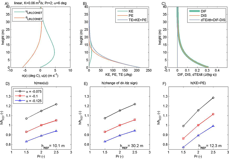
Figure 1. Vertical profiles of potential temperature θ and wind speed u in the linear solution of the Prandtl model for the katabatic flow (A), corresponding kinetic energy KE, potential energy PE and total energy TE (B), and diffusion DIF, dissipation DIS and storage terms ∂TE/∂t (C). The height of the low-level jet h_j (D), height of the stability change (E) and height at which KE becomes larger than PE (F) as function of Prandtl number Pr (x axis) and slope angle α (different color). Heights in (D–F) are relative to the reference heights h_REF from the solutions when Pr = 2 and α = −0.1 rad.

The following three heights are of interest to us:

(1) The height of the low-level jet h_j. This is the maximum of u(z) which occurs at h_j = π/4 h_P in the linear solutions, i.e., it increases with increasing Pr and decreases with an increasing slope (see also, Figure 1D). At the same time, the maximum u_LIN is insensitive to the slope angle and decreases with increasing Pr (this can be shown by inserting h_j in Equation 5) as is confirmed in Figure S3.1A (please note that lines are shifted by the amount ±0.5 from the reference slope angle for presentation purposes).

(2) The depth of the stable (in the anabatic case, unstable) layer. At the top of the stable layer dθ/dz = 0, and this height equals 3 h_P. It also increases with increasing Pr and decreases with an increasing slope in the linear solution (Figure 1E).

(3) The level where KE starts to dominate over PE (TE is primarily governed by PE close to the surface, while KE becomes larger than PE somewhere above h_j). For the linear solutions of katabatic (and anabatic) flow, one can show (by setting the condition KE/PE = 1) that the height where KE starts to dominate equals h_P cos⁻¹([1/(1 + Pr)]^1∕2); i.e., it also increases with increasing Pr and decreases with an increasing slope angle (Figure 1F). This level is directly linked, though in a nonlinear way, to the gradient Richardson number, which is significantly smaller than 1, and the consequent onset of dynamic flow instabilities (e.g., Grisogono 2003). At the same time, the amplitude at which KE starts to dominate is insensitive to the choice of slope (Figure S3.1E; lines are shifted by the amount ±0.5 from the reference slope angle for presentation purposes). This behavior of the KE is by definition directly linked to the behavior of u_LIN. More details about this measure are presented in Supplementary Materials 2.

(b) Nonlinear case

The deviation of the nonlinear from the linear solution for katabatic flow is presented in Figure 2. The general characteristics of θ_NOLIN and u_NOLIN profiles are equivalent to θ_LIN and u_LIN, and their corresponding KE, PE, and TE profiles are also similar. The nonlinear solution has slightly lower wind speeds and higher potential temperature (i.e., lower potential temperature anomalies; Figure 2A) and this leads to lower KE, PE, and TE (Figure 2B). However, the vertical profiles of DIS and DIF do not overlap as in linear cases and are slightly larger in the nonlinear case (Figure 2C). Also, in the nonlinear case, the interaction term INT is present. Its amplitude is much lower than the other two governing terms in the energy equation. More importantly, the TE storage term is nonzero and this will be discussed later, in Section Discussion.

FIGURE 2

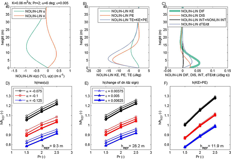
Figure 2. (A–C) Differences between nonlinear and linear (Figure 1) solutions of the (extended) Prandtl model (cf. Grisogono et al., 2015). (D–F) are equivalent to (D–F) in Figure 1. Also, sensitivity to the nonlinearity parameter ε (with increasing line thickness as ε is increased) is included in (D–F), while (C) includes the vertical profile of the interaction term INT that is equal to zero in the linear case. The reference heights h_REF are based on the solutions when Pr = 2, α = −0.1 rad and ε = 0.005.

We also examine the sensitivity of the nonlinear solution to the choices of Pr and α. Additionally, we examine the impact of the nonlinearity term ε, starting with ε = 0.005 and modifying this value by ±25%. Nonlinear effects have the lowest impact on variability in the ensemble of 27 solutions of the weakly nonlinear Prandtl model when compared to the other two governing parameters (Figures 2D–F). The general behavior of the nonlinear solution is similar to that of the linear solution, except that the maximum u_NOLIN (and the corresponding maximum KE) is moderately reduced for larger slopes (while the maximum u_LIN is constant; cf. Figures S3.1A,E vs. Figures S3.1B,F). This aspect of the low-level jet in the nonlinear solution is shared by LES simulations in e.g., Grisogono and Axelsen (2012) and will be explored in future studies. The increase in ε reduces all three heights (Figures 2D–F) and amplitudes of the maximum wind speed and KE (Figures S3.1B,F).

Anabatic Flow

In this subsection we present a general overview of anabatic flow solutions from the linear and weakly nonlinear Prandtl model. The main difference when compared to katabatic flow is the existence of the surface temperature surplus that induces the anabatic flow (now +6 K; cf. Defant, 1949). This change in the surface boundary condition is related to the corresponding increase in eddy heat conductivity from K = 0.06 m²/s to K = 3.0 m²/s and the increase of the nonlinearity parameter from ε = 0.005 to ε = 0.03, as explained in Grisogono et al. (2015): since max(ε)~γ h_P/ |C|, then ε_Anabatic/ε_Katabatic ~ (K_Anabatic/K_Katabatic)^1/2. With this choice of ε, perturbations to the linear solution are present, but the general structure of the solution does not change. Although anabatic upslope winds are generally deeper than typical katabatic flows, in our comparisons the same amplitude of potential temperature deviations at the surface is set so that the same potential energy of the slope flow PE is found at the surface. This is also reflected in the similar range of amplitudes of the analyzed measures in subsections Katabatic Flow and Anabatic Flow, but for anabatic flow the maximum values of the analyzed heights are typically an order of magnitude larger.

(a) Linear case

The vertical profiles of the upslope wind u_LIN, potential temperature deviations θ_LIN, KE, PE, and TE, and, finally, the terms in the total energy equation related to diffusion DIF, dissipation DIS and local storage ∂TE/∂t of TE are shown in Figures 3A–C. All vertical profiles are equivalent to their katabatic counterpart in terms of the general structure (cf. Figure 1). The sensitivity of the low-level jet height, the level where the change in the local static stability occurs, and the level where KE starts to dominate over PE are equivalent to those in the linear katabatic case (cf. Figures 1D–F vs. Figures 3D–F).

FIGURE 3

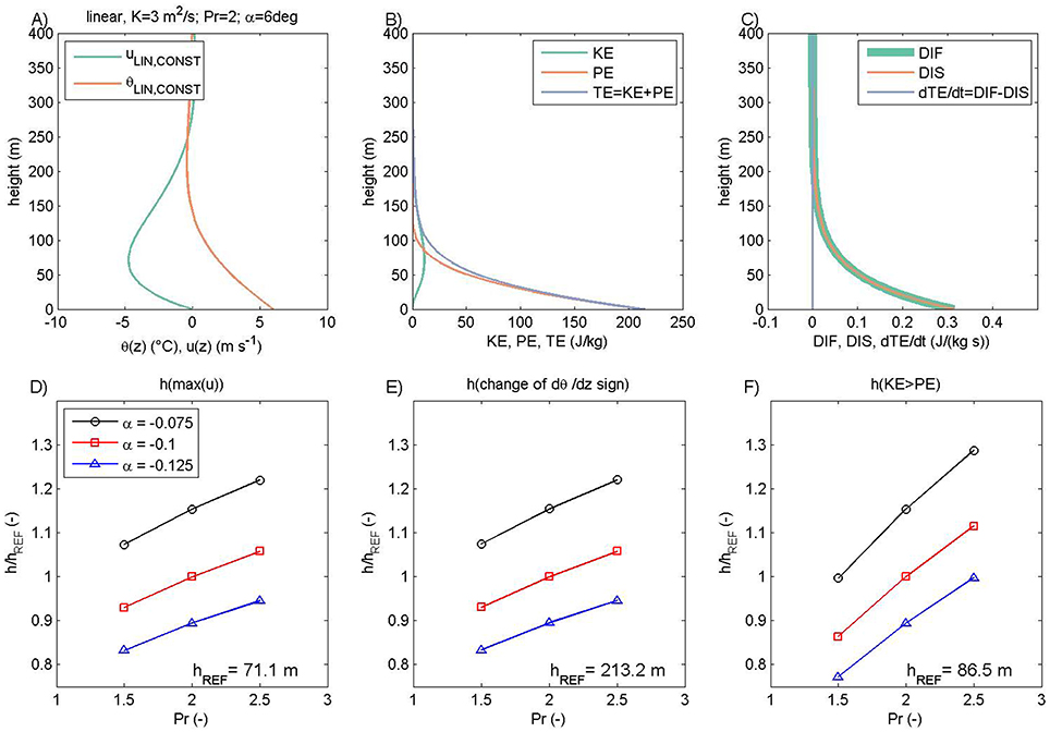
Figure 3. Same as Figure 1 but for anabatic flow.

(b) Nonlinear case

The nonlinear solution of anabatic flow is described in this subsection. When compared to its katabatic counterpart, the vertical profiles of along-the-slope wind speed and potential temperature have the same general structure and this is also the case for kinetic, potential and total energy of the nonlinear vs. linear solution. However, all three energy components (KE, PE, and TE) are increased in the nonlinear anabatic solution, when compared to the linear solution (Figure 4B). This is a consequence of the increased wind speeds (in absolute terms) and increased potential temperature of anabatic flow (Figure 4A). As for the linear case of anabatic flow, the nonlinear anabatic flow is extended over a deeper layer, so both the low-level jet and inversion height are higher than in the corresponding katabatic flow. As discussed later, the increase in the basic ε up to ε = 0.03 is the reason for the substantial rise in the magnitude of the interaction INT and total energy TE local storage terms ∂TE/∂t (Figure 4C). In contrast to katabatic flow, the TE diffusion DIF now departs from the dissipation DIS toward lower values. Also, while in katabatic flow the small amplitude of INT and the imbalance between DIF and DIS makes ∂TE/∂t become nonzero, in anabatic flow it is the sign and amplitude of the interaction term INT that dominates the production of TE.

FIGURE 4

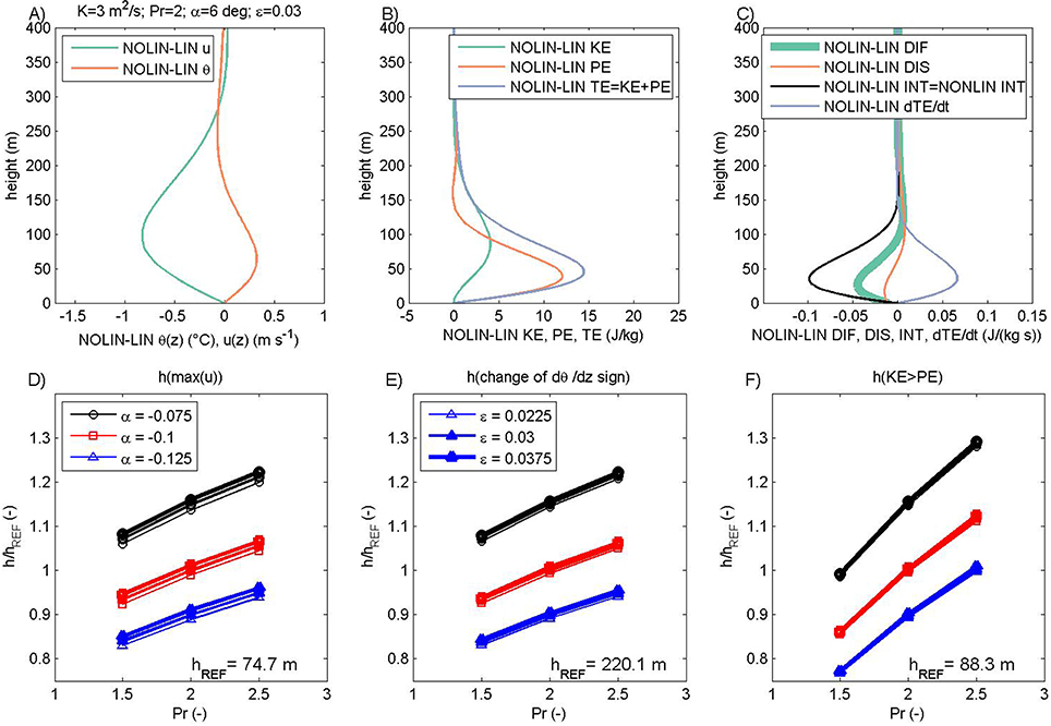
Figure 4. Same as Figure 2 but for anabatic flow and ε = 0.03.

The sensitivity of the selected height measures to Pr and slope angle is the same as for the linear anabatic case (and also for both katabatic types of solutions; Figures 4D–F). The main difference is found concerning the selection of ε. In contrast to the katabatic nonlinear case, in the anabatic nonlinear case the increase in ε leads to: (1) a rise in the low-level jet height and speed (Figure 4D), (2) a rise in the inversion height (in anabatic flow a transition occurs from statically unstable to stable conditions) that is not substantial for the selected range of control parameters (Figure 4E), (3) low sensitivity of the height where KE dominates over PE to the nonlinearity parameter ε (which can be neglected for the purposes of this study; Figure 4F).

Common to all previous solutions, while the maximum in KE is attained at levels of maximum along-the-slope wind speed, KE becomes larger than PE above this level of maximum KE (cf. Figure 4F vs. Figure 5D). At the same time, the amplitude at which KE starts to dominate increases slightly as the slope increases (Figure S3.1H). The increase in ε also increases the amplitude of KE where it becomes larger than PE (in contrast to katabatic nonlinear flow), and this sensitivity to ε is comparable to the sensitivity to the slope angle α (Figure S3.1H). In summary, KE dominates over PE above h_pcos⁻¹[1/(1+Pr)^1∕2] and this height is usually between h_j and 2 h_j. It is related to the corresponding gradient Richardson number, which compares the vertical gradients of PE vs. KE. When the Richardson number falls substantially below 1, dynamic instabilities might occur in the corresponding sublayer (see also Supplementary Materials 2).

FIGURE 5

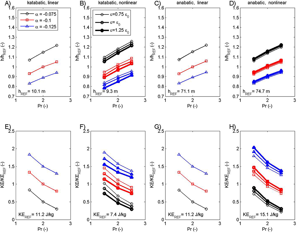
Figure 5. The height of the maximum of kinetic energy KE (A–D) and the maximum KE value (E–H) for katabatic (A,B,E,F) and anabatic (C,D,G,H), linear (A,C,E,G), and nonlinear (B,D,F,H) cases. Selected measures are determined as functions of the Prandtl number Pr (x axis), slope angle α (different line color) and nonlinearity parameter ε (different line thickness) in the case of nonlinear solutions. Heights in (A–D) are relative to the corresponding h_REF. For presentation purposes, the lines in (E–H) are shifted ±0.5 from the referentce α = −0.1 line (otherwise, exact overlap is present in (E,G), and approximate overlap is present in (F,H).

Energetics: Katabatic and Anabatic Flows

The potential energy maximum (PEmax) and total energy maximum (TEmax) are found at the lowest level in linear and nonlinear solutions for both anabatic and katabatic flows (insensitive to the choice of α, Pr, and ε). Also, the amplitude of PEmax and TEmax equals 215.4 J/kg in all cases (Figures 1–4, panel B). The same amplitude of PEmax and TEmax in both katabatic and anabatic flows is a result of the same temperature anomaly at the surface (but with a different sign, i.e., ± 6 K in this study).

At the same time, the kinetic energy maximum (KEmax) is sensitive to choices in our parameter space and set of solutions (Figure 5). The height of KEmax (equivalent to the low-level jet height h_j) increases when Pr varies from Pr = 1.5 to Pr = 2.5, and it decreases when |α| is increased (Figures 5A–D). In the case of katabatic flow, the height of KEmax is within a similar range for both the linear (Figure 5A) and nonlinear case (the solutions are only slightly sensitive to ε; Figure 5B). In the case of anabatic flows, a similar structure of solutions is found, only over deeper layers than for katabatic flows (Figure 5C). While all solutions behave in a consistent way with respect to Pr and α, there is a contrasting response to the increase in ε in nonlinear solutions: as ε is increased, the height and amplitude of KEmax reduce in katabatic flow (Figures 5B,F), while they rise in anabatic flow (Figures 5D,H). The latter contrast occurs because the low-level jet height and amplitude, i.e., h_j and u_max, show a similar sensitivity to ε. Grisogono et al. (2015) showed that an ε increase leads to an h_j and u_max decrease in the nonlinear katabatic solution, and an h_j and u_max increase in the nonlinear anabatic solution.

The amplitude of KEmax in linear solutions (both katabatic and anabatic) is the only function of the Pr (it collapses to approximately the same values for different slopes and, more interestingly, the same structure is present for both katabatic and anabatic solutions; Figures 5E,G for presentation purposes the lines are shifted ±0.5 from the reference slope angle). However, in the nonlinear case, sensitivity to all three parameters is present: (1) the reduction of KEmax with increasing Pr, which is classical Prandtl model behavior, (2) the reduction of KEmax when increasing α and ε in katabatic flow (Figure 5F), as explained just above, but (3) an increase in KEmax when increasing the nonlinearity in anabatic flow (Figure 5H). The sensitivity of KEmax to Pr and α is expected from the formulation of KEmax in the linear solution (Equation 5) and the similarity of the linear and nonlinear vertical profiles.

The diffusion maximum (DIFmax) and dissipation maximum (DISmax) are found at the surface level in linear and nonlinear solutions for both anabatic and katabatic flows (insensitive to the choice of α, Pr, and ε). This is the simple consequence of the more intense wind and temperature vertical changes near the slope surface. In contrast to PEmax and TEmax, and similar to KEmax, the amplitude of both DIFmax and DISmax is sensitive to the Prandtl number Pr, slope angle α and the nonlinearity parameter ε: DIFmax and DISmax (1) reduce when Pr increases, (2) increase when the slope increases, and (3) are only slightly sensitive to increasing ε. DIFmax and DISmax vary in a common range in the linear and nonlinear solutions for both anabatic and katabatic flows (Figure S3.2).

In the case of nonlinear solutions for anabatic and katabatic flow, the additional interaction term is present. Both the amplitude and height of the interaction term maximum INTmax are functions of all three parameters (see Figures 6A,B for INTmax height and Figures 6E,F for INTmax amplitude). The sensitivity of the amplitude and height of INTmax shows a behavior similar to KEmax: in katabatic flow, the height of INTmax varies from ~3 m to ~5 m, while in anabatic flow from ~28 m to ~43 m. Also, INTmax varies from ~1·10⁻³ J/kg/s to ~4·10⁻³ J/kg/s in katabatic flow, while it is negative and varies from ~ −0.22 J/kg/s to ~ -0.04 J/kg/s in anabatic flow. Also, by examining the maximum of the triple product in INT (Equation 3), one can estimate the height where INTmax occurs: this is approximately 4/9 h_j (this result can be derived by using the linear solutions to find numerically the local maximum of the triple product; a more precise estimation would include the use of the nonlinear solutions u_NOLIN and θ_NOLIN). This means that INTmax, i.e., the maximum of the slope-normal transport of potential energy, occurs at about ½ h_j, which is one of the new results of this study.

FIGURE 6

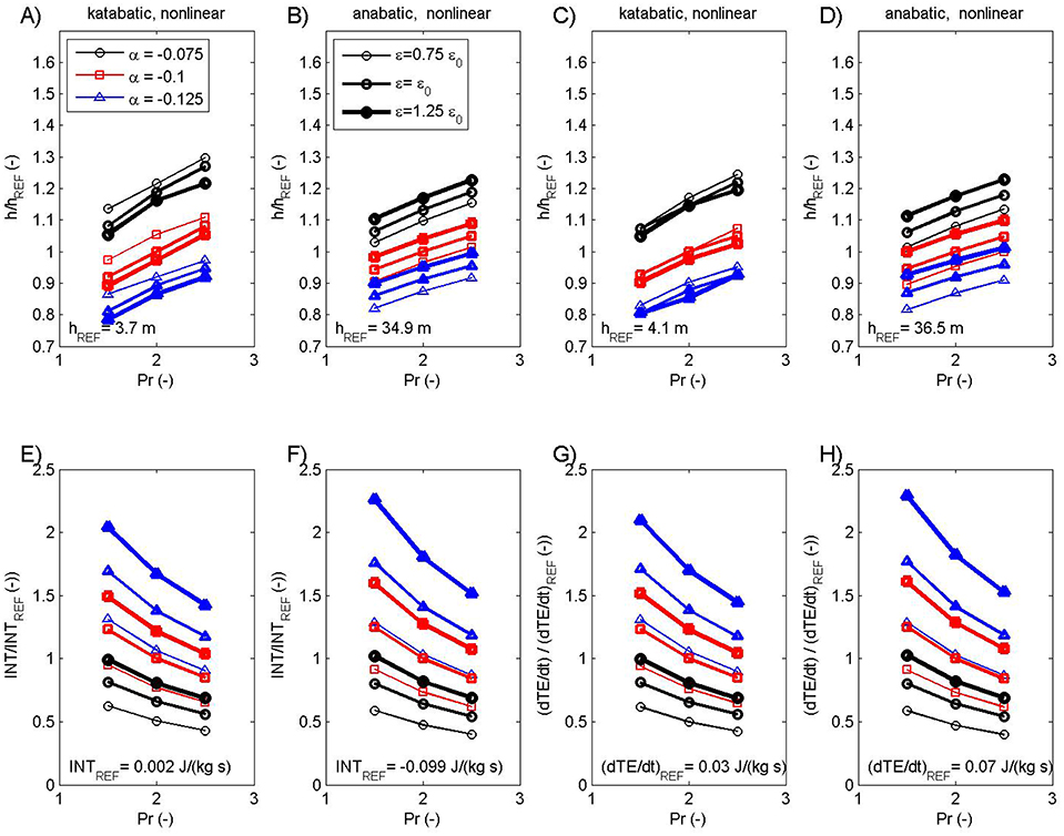
Figure 6. The height of the maximum of the interaction term INT (A,B), the height of the maximum of the storage term ∂TE/∂t (C,D), the maximum INT value (E,F) and the maximum ∂TE/∂t value (G,H) for katabatic (A,C,E,G) and anabatic (B,D,F,H) nonlinear cases. Selected measures are determined as functions of Prandtl number Pr (x axis), slope angle α (different color) and nonlinearity parameter ε (different line thickness). Values in panels are relative to the corresponding h_REF (A–D), INT_REF (E,F) and ∂TE/∂t_REF(G,H).

The last quantity examined in this subsection is the tendency of total energy ∂TE/∂t. In linear solutions for anabatic and katabatic flow, this quantity is zero, reflecting the stationarity of our solutions by definition. However, in nonlinear solutions, the diffusion, dissipation and interaction terms do not balance, so ∂TE/∂t can attain nonzero values. For nonlinear katabatic flow, and based on the specific selection of model parameters, maximum values of ∂TE/ ∂t range from ~0.01 J/kg/s to ~0.07 J/kg/s at heights reaching from ~3 m to ~5 m (Figures 6C,G). The amplitude/height of maximum ∂TE/ ∂t in the katabatic solution decreases/increases with increasing Pr, increases/decreases with increasing α (because | INT | ~|α|), and increases/decreases with increasing ε (Figures 6C,G). For the nonlinear anabatic flow, maximum values of ∂TE/∂t range from ~0.03 J/kg/s to ~0.15 J/kg/s at heights ranging from ~30 m to ~45 m (Figures 6D,H). The amplitude and height of maximum ∂TE/∂t in the anabatic solution behave in a similar manner as in their katabatic counterpart (Figures 6D,H). The only difference is found for the case of the height of maximum ∂TE/∂t, where now an ε increase is linked with a ∂TE/∂t increase. Again, nonzero profiles of ∂TE/∂t, due to nonlinearity, imply that the stationarity of solutions is not satisfied, and depends on the joint effect of DIF, DIS, and INT terms.

Discussion

In this section, we briefly discuss some of the results where references to LES studies and the issue of the non-stationarity present in our weakly nonlinear solutions are addressed.

The reduction of h_j with an increasing slope is a well-known feature of katabatic flows (in both LES results and the Prandtl model, see e.g., Grisogono and Axelsen, 2012). Also, with increasing Pr, katabatic flow is characterized by an increase in the momentum mixing when compared to the heat mixing, pushing and spreading the low-level jet upwards. At the same time, the maximum u_LIN is insensitive to the choice of slope angle but reduces for increasing Pr (Figure S3.1A; cf. Grisogono and Axelsen, 2012). However, in LES simulations (in contrast to the classical Prandtl model) the maximum u reduces with an increasing slope angle. This is also found in the nonlinear solution of our extended Prandtl model. Future studies may explore the behavior of the LES and nonlinear solutions in detail.

Conceptually, there are no crucial differences (besides the vertical extent) in KE, PE, and TE in anabatic and katabatic flows, since all energy measures are quadratic quantities and the same amplitude of the temperature deficit/surplus is set as a lower boundary condition. For both the anabatic and katabatic nonlinear solutions, variability due to perturbations in ε is lower than variability due to the Pr and α. The actual range of ε is discussed in detail in Grisogono et al. (2015; their subsection 2.3). In short, the value of ε should not introduce first-order corrections that modify the general structure of the zero-order solutions, and this is also confirmed by our study in terms of TE, PE, and TE.

Another important difference between the linear and nonlinear katabatic (and anabatic) solutions is the nonzero ∂TE/∂t in the nonlinear case. In terms of the interaction between wind speed and potential temperature with the background atmosphere, the absolute value of the interaction term, i.e., |INT| decreases with increasing Pr. This indicates a weaker coupling between the turbulent mixing of momentum and heat, i.e., a decrease of the slope-normal transport of potential energy; hence, the covariance between wind speed and temperature in INT weakens (note that the latter term is made of a triplet product). At the same time, as |INT| decreases with increasing Pr, ∂TE/∂t also weakens with increasing Pr. The existence of nonzero ∂TE/∂t in the nonlinear solution indicates deviations from stationarity of the total energy in the system, and reflects a leakage of energy from the background atmosphere to slope flows. It may be expected that in a more realistic flow there would be interplay among the energy terms, yielding a quasi-periodic behavior and generation of waves (most jets are unstable to small perturbations). In a more realistic model, which would allow not only for time dependency but also for vertical velocity—pressure covariance, the kind of imbalance that we found in this study would immediately generate wave-like perturbations (e.g., Stiperski et al., 2007; Zhong and Whiteman, 2008; Axelsen, 2010; Largeron et al., 2010; Sun et al., 2015). Furthermore, this suggests that an extended and more comprehensive model than that presented in Grisogono et al. (2015) should allow for time dependency and/or velocity—pressure covariance. Also, slight to moderate imbalance among the energy terms in this nonlinear model may suggest that there is perhaps no real steady-state nonlinear slope flow; thus, excursions from pure steadiness could occur in nonlinear thermally driven flows. To add a point, Axelsen (2010; his Figures 3.5, 3.6) shows with an LES that pure katabatic flow is unsteady even under idealized conditions (constant slope, etc.). In his idealized simulation, internal and external gravity-wave modes are launched from the low-level katabatic jet. In short, the existence of non-stationarity in the nonlinear solution may reflect real non-stationarity in nonlinear models, LES simulations and observations, and/or limitations in the extended Prandtl model, where for the latter an inclusion of the additional nonlinear term in the momentum equation might close the energy budget. Again, this will require future study.

Lastly, the question is how the results of this study are comparable to the real atmosphere. While high-resolution observations over long gentle slopes and specific background atmospheric conditions are hard to acquire, we estimate KE, PE, and TE from the PASTEX-94 observations of glacier wind (van den Broeke, 1997a,b; Oerlemans and Grisogono, 2002; Figure S3.3). These results should only be considered indicative, but they do show the dominance of PE near the sloped surface, and the elevated maximum of KE, followed by the level where KE starts to dominate over PE (Figure S3.3B): all in accordance with our analysis of linear and nonlinear energetics of the (extended) Prandtl model. Interestingly, for this observation case DIF and DIS do not balance either, so nonzero ∂TE/∂t is found (Figure S3.3C). The latter result suggests the existence of either nonlinear effects or other important processes in the real atmosphere, which are not taken into account in our model. However, for stronger claims and conclusions, much larger observational datasets need to be analyzed and a more comprehensive evaluation must be performed.

Summary and Conclusions

In this study, we have evaluated the energetics of the linear and weakly nonlinear solutions of the (extended) Prandtl model from Grisogono et al. (2015). From an ensemble of solutions where three controlling parameters were perturbed (i.e., the Prandtl number Pr, the slope angle α and the nonlinearity parameter ε), KE, PE, and TE profiles were estimated for both katabatic and anabatic flows. Also, the governing terms in the prognostic total energy equation were examined in four groups of solutions (linear/nonlinear, katabatic/anabatic).

The nonlinearity effect induced small to moderate variations in the total energy TE. These variations caused the non-stationarity of TE, which is in conflict with the initially assumed stationarity of along-the-slope wind speed and potential temperature. This suggests the need for joining nonlinear and time-dependent effects in katabatic/anabatic flow as a way of circumventing the limitations of the weakly nonlinear Prandtl model as developed by Grisogono et al. (2015). At the same time, the maximum of the wind speed (and kinetic energy) in the nonlinear solution is found to be sensitive to the slope angle (this is not present in the linear solution), and is in this way comparable to LES simulations in e.g., Grisogono and Axelsen (2012). Since the time-dependent solution to the linear Prandtl model is already quite complicated (e.g., Grisogono, 2003; Zardi and Serafin, 2014), it seems unlikely that a corresponding weakly nonlinear time-dependent analytic solution to the problem could be found in an elegant form. Yet, there are indications that there might be no steady-state nonlinear solution to thermally driven slope flows (Axelsen, 2010), which agrees with our findings.

We have limited our analysis to the energy terms and prognostic total energy equation of the mean slope flow only. It is shown that the strongest interaction between the θ- and u- profiles occurs at a height of around 4/9 h_j, with h_j = π/4 h_p, i.e., about half the height of the low-level jet. Moreover, kinetic energy dominates over potential energy above h_pcos⁻¹[1/(1 + Pr)^1∕2], which is typically between h_j and 2 h_j. Thus, this is the sublayer where dynamic instabilities might occur. It is directly, although nonlinearly, related to the corresponding gradient Richardson number, which compares the differential change of potential energy vs. kinetic energy of the flow. This number falls significantly below 1 in that sublayer. However, the height where KE starts to dominate over PE is not the height of the maximum KE. The latter is trivially the same as the height of the low-level jet, and always below the height where KE>PE.

A more complete energy framework would include an estimation of the potential and kinetic energy contributions from the basic state, turbulence and possibly mesoscale components (e.g., waves) in the system. Since there is still no satisfactory approach that would include the effects of sub-grid slope flows in the form of parameterizations in mesoscale and large-scale weather and climate models, greater effort should be made in order to increase the applicability of these types of models in complex orography regions (e.g., Bornemann et al., 2010).

Finally, the results of our simple small-ensemble exercise may be compared with observations (where care is needed to ensure high-resolution measurements in order to correctly estimate the first and second vertical derivatives in the total energy equation). A second approach to an independent evaluation of our analytical model includes the construction of the total energy budget from an ensemble of LES simulations (e.g., Grisogono and Axelsen, 2012), where non-stationarity and energetics of katabatic and anabatic flows can be further explored.

Author Contributions

All authors listed, have made substantial, direct and intellectual contribution to the work, and approved it for publication.

Funding

IG was supported by the Croatian Science Foundation, CARE project, No. 2831; IM, ŽV, and BG were supported by the Grant Agency of the Czech Science Foundation under the GAČR project 14-12892S and by the Croatian Science Foundation, CATURBO project, No. 09/151.

Conflict of Interest Statement

The authors declare that the research was conducted in the absence of any commercial or financial relationships that could be construed as a potential conflict of interest.

Acknowledgments

The authors wish to thank the reviewers and the editor for providing detailed and constructive comments that have substantially improved the initial versions of the paper.

Supplementary Material

The Supplementary Material for this article can be found online at: https://www.frontiersin.org/article/10.3389/feart.2016.00072

References

Axelsen, S. L. (2010). Large-Eddy Simulation and Analytical Modeling of Katabatic Winds. Ph.D., dissertation, IMAU, Utrecht University, the Netherlands, 164.

Bender, C. M., and Orszag, S. A. (1978). Advanced Mathematical Methods for Scientists and Engineers. New York, NY: McGraw-Hill Book Company.

Google Scholar

Bornemann, J., Lock, A., Webster, S., Edwards, J., Weeks, M., Vosper, S., et al. (2010). “Understanding cold valleys in convective scale models,” in 32nd EWGLAM and 17th SRNWP Meetings. Available online at: srnwp.met.hu/Annual_Meetings/2010/ (Accessed 07-01-2016)

Burkholder, B. A., Shapiro, A., and Fedorovich, E. (2009). Katabatic flow induced by a cross-slope band of surface cooling. Acta Geophys. 57, 923–949. doi: 10.2478/s11600-009-0025-6

CrossRef Full Text | Google Scholar

DeCaria, A. J. (2007). Relating static energy to potential temperature: a caution. J. Atmos. Sci. 64, 1410–1412. doi: 10.1175/JAS3906.1

CrossRef Full Text | Google Scholar

Defant, F. (1949). Zur theorie der Hangwinde, nebst bemerkungen zur Theorie der Berg- und Talwinde. Arch. Meteor. Geophys. Biokl. Ser. A1, 421–450. doi: 10.1007/BF02247634

CrossRef Full Text | Google Scholar

Fedorovich, E., and Shapiro, A. (2009a). Structure of numerically simulated katabatic and anabatic flows along steep slopes. Acta Geophys. 57, 981–1010. doi: 10.2478/s11600-009-0027-4

CrossRef Full Text | Google Scholar

Fedorovich, E., and Shapiro, A. (2009b). Turbulent natural convection along a vertical plate immersed in a stably stratified fluid. J. Fluid Mech. 636, 41–57. doi: 10.1017/S0022112009007757

CrossRef Full Text | Google Scholar

Fernando, H., Pardyjak, E., Di Sabatino, S., Chow, F., De Wekker, S., Hoch, S., et al (2015). THE MATERHORN - unraveling the intricacies of mountain weather. Bull. Am. Meteorol. Soc. 96, 1945–1967. doi: 10.1175/BAMS-D-13-00131.1

CrossRef Full Text | Google Scholar

Grachev, A. A., Leo, L. S., Di Sabatino, S., Fernando, H. J. S., Pardyjak, E. R., and Fairall, C. W. (2015). Structure of turbulence in katabatic flows below and above the wind-speed maximum. Boundary Layer Meteorol. 159, 469–494. doi: 10.1007/s10546-015-0034-8

CrossRef Full Text | Google Scholar

Grisogono, B. (2003). Post-onset behaviour of the pure katabatic flow. Boundary Layer Meteorol. 107, 157–175. doi: 10.1023/A:1021511105871

CrossRef Full Text | Google Scholar

Grisogono, B., and Axelsen, S. L. (2012). A note on the pure katabatic wind maximum over gentle slopes. Boundary Layer Meteorol. 145, 527–538. doi: 10.1007/s10546-012-9746-1

CrossRef Full Text | Google Scholar

Grisogono, B., Jurlina, T., Večenaj, Ž., and Güttler, I. (2015). Weakly nonlinear Prandtl model for simple slope flows. Q. J. R. Meteorol. Soc. 141, 883–892. doi: 10.1002/qj.2406

CrossRef Full Text | Google Scholar

Grisogono, B., and Oerlemans, J. (2001). A theory for the estimation of surface fluxes in simple katabatic flows. Q. J. R. Meteorol. Soc. 127, 2725–2739. doi: 10.1002/qj.49712757811

CrossRef Full Text | Google Scholar

Holtslag, A. A. M., Svensson, G., Baas, P., Basu, S., Beare, B., Beljaars, A. C. M., et al. (2013). Stable atmospheric boundary layers and diurnal cycles: challenges for weather and climate models. Bull. Am. Meteorol. Soc. 94, 1691–1706. doi: 10.1175/BAMS-D-11-00187.1

CrossRef Full Text | Google Scholar

Largeron, Y., Staquet, C., and Chemel, C. (2010). Turbulent mixing in a katabatic wind under stable conditions. Meteorol. Z. 19, 467–480. doi: 10.1127/0941-2948/2010/0346

CrossRef Full Text | Google Scholar

Mahrt, L. (1998). Stratified atmospheric boundary layers and breakdown of models. Theoret. Comput. Fluid Dyn. 11, 263–279. doi: 10.1007/s001620050093

CrossRef Full Text | Google Scholar

Mahrt, L. (2014). Stably stratified atmospheric boundary layers. Annu. Rev. Fluid Mech. 46, 23–45. doi: 10.1146/annurev-fluid-010313-141354

CrossRef Full Text | Google Scholar

Mauritsen, M., Svensson, G., Zilitinkevich, S. S., Esau, I., Enger, L., and Grisogono, B. (2007). A total turbulent energy closure model for neutrally and stably stratified atmospheric boundary layers. J. Atmos. Sci. 64, 4113–4126. doi: 10.1175/2007JAS2294.1

CrossRef Full Text | Google Scholar

Oerlemans, J., and Grisogono, B. (2002). Glacier wind and parameterization of the related surface heat flux. Tellus 54A, 440–452. doi: 10.1034/j.1600-0870.2002.201398.x

CrossRef Full Text | Google Scholar

Poulos, G., and Zhong, S. (2008). An observational history of small-scale katabatic winds in mid-latitudes. Geogr. Compass 2, 1798–1821. doi: 10.1111/j.1749-8198.2008.00166.x

CrossRef Full Text | Google Scholar

Prandtl, L. (1942). Führer durch die Strömungslehre. Braunschweig: Vieweg and Sohn, 648.

Google Scholar

Princevac, M., and Fernando, H. J. S. (2007). A criterion for the generation of turbulent anabatic flows. Phys. Fluids. 19, 105102. doi: 10.1063/1.2775932

CrossRef Full Text | Google Scholar

Sandu, I., Beljaars, A., Bechtold, P., Mauritsen, T., and Balsamo, G. (2013). Why is it so difficult to represent stably stratified conditions in numerical weather prediction (NWP) models? J. Adv. Model. Earth Syst. 5, 117–133. doi: 10.1002/jame.20013

CrossRef Full Text | Google Scholar

Shapiro, A., Burkholder, B., and Fedorovich, E. (2012). Analytical and numerical investigation of two-dimensional katabatic flow resulting from local surface cooling. Boundary Layer Meteorol. 145, 249–272. doi: 10.1007/s10546-011-9685-2

CrossRef Full Text | Google Scholar

Shapiro, A., and Fedorovich, E. (2008). Coriolis effects in homogeneous and inhomogeneous katabatic flows. Q. J. R. Meteorol. Soc. 134, 353–370. doi: 10.1002/qj.217

CrossRef Full Text | Google Scholar

Shapiro, A., and Fedorovich, E. (2014). A boundary-layer scaling for turbulent katabatic flow. Boundary Layer Meteorol. 153, 1–17. doi: 10.1007/s10546-014-9933-3

CrossRef Full Text | Google Scholar

Skyllingstad, E. D. (2003). Large-eddy simulation of katabatic flows. Boundary Layer Meteorol. 106, 217–243. doi: 10.1023/A:1021142828676

CrossRef Full Text | Google Scholar

Smith, C. M., and Porté-Agel, F. (2013). An intercomparison of subgrid models for large eddy simulation of katabatic flows. Q. J. R. Meteorol. Soc. 140, 1294–1303. doi: 10.1002/qj.2212

CrossRef Full Text | Google Scholar

Smith, C. M., and Skyllingstad, E. D. (2005). Numerical simulation of katabatic flow with changing slope angle. Monthly Weather Rev. 133, 3065–3080. doi: 10.1175/MWR2982.1

CrossRef Full Text | Google Scholar

Stiperski, I., Kavčič, I., Grisogono, B., and Durran, D. R. (2007). Including Coriolis effects in the Prandtl model for katabatic flows. Q. J. R. Meteorol. Soc. 133, 101–106. doi: 10.1002/qj.19

CrossRef Full Text | Google Scholar

Sun, J., Nappo, C. J., Mahrt, L., Belušić, D., Grisogono, B., Stauffer, D. R., et al. (2015). Review of wave-turbulence interactions in the stable atmospheric boundary layer. Rev. Geophys. 53, 956–993. doi: 10.1002/2015RG000487

CrossRef Full Text | Google Scholar

van den Broeke, M. R. (1997a). Structure and diurnal variation of the atmospheric boundary layer over amid-latitude glacier in summer. Boundary Layer. Meteorol. 83, 183–205.

Google Scholar

van den Broeke, M. R. (1997b). Momentum, heat and moisture budgets of the katabatic wind layer over amid-latitude glacier in summer. J. Appl. Meteorol. 36, 763–774.

Google Scholar

Zammett, R. J., and Fowler, A. C. (2007). Katabatic winds on ice sheets: a refinement of the Prandtl model. J. Atmos. Sci. 64, 2707–2716. doi: 10.1175/JAS3960.1

CrossRef Full Text | Google Scholar

Zardi, D., and Serafin, S. (2014). An analytic solution for time-periodic thermally driven slope flows. Q. J. R. Meteorol. Soc. 141, 1968–1974. doi: 10.1002/qj.2485

CrossRef Full Text | Google Scholar

Zardi, D., and Whiteman, C. D. (2013). “Diurnal mountain wind systems,” in Mountain Weather Research and Forecasting, eds F. K. Chow, S. F. J. de Wekker, and B.-J. Snyder (Dordrecht: Springer), 35–119.

Zhong, S., and Whiteman, C. D. (2008). Downslope flows on a low-angle slope and their interactions with valley inversions. Part II: numerical modeling. J. Appl. Meteorol. Climatol. 47, 2039–2057. doi: 10.1175/2007JAMC1670.1

CrossRef Full Text | Google Scholar