Accumulation Rates during 1311–2011 CE in North-Central Greenland Derived from Air-Borne Radar Data

1. Introduction

Knowledge of past accumulation is essential for studying the evolution of ice sheets and their response to climate change. Estimates of past accumulation rates are often based on ice-core records that represent point measurements rather than spatially distributed observations. Unfortunately, ice core measurements of accumulation rates remain sparse, especially in remote areas such as central Greenland. Here, we present the accumulation pattern over the last seven centuries for an area encompassing two deep ice-core locations: the NEEM (North Greenland Eemian Ice Drilling, 77.45°N, 51.06°W) and the NGRIP (North Greenland Ice Core Project, 75.1°N, 42.32°W) ice-core drill sites.

The specific surface mass balance (SMB) and its spatial distribution is a key parameter for elucidating total ice sheet mass balance. In order to retrieve the SMB, studies have employed various approaches such as firn cores and/or snow pit studies at times combined with weather station data (e.g., Ohmura and Reeh, 1991; Bales et al., 2001, 2009), and climate models (e.g., Ettema et al., 2009; Burgess et al., 2010; Hanna et al., 2011; Box et al., 2013). Regardless of the approach, the estimated accumulation rates of the Greenland Ice Sheet (GrIS) display the same overall pattern: high rates on the coast and low rates in the interior. The location of the ice divide influences the SMB, especially in central northern Greenland, since it marks the highest points in the interior of the ice sheet (see Figure 1, inset). For this region, Ohmura and Reeh (1991) showed that the ice divide acts as a topographic barrier for water vapor transported from the west coast. Numerous studies have confirmed that this topographic barrier results in high accumulation rates on the west coast, decreasing rates as the elevation rises toward the interior, and very low accumulation rates east of the ice divide (e.g., Bales et al., 2001; Ettema et al., 2009; Burgess et al., 2010; Box et al., 2013). Similar gradients in accumulation rates have been observed across ice divides in Antarctica (Neumann et al., 2008; Koutnik et al., 2016). Another example of elevation-controlled SMB is the ice rises in coastal East Antarctica (Lenaerts et al., 2014), although they are of a substantially smaller spatial scale (a few tens of kilometers).

FIGURE 1

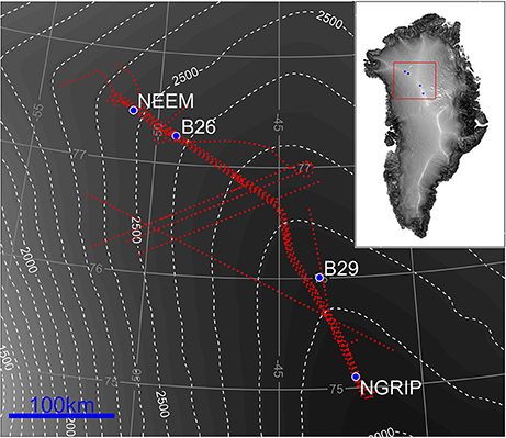
Figure 1. Location of radar data used in this study (red lines) and the locations of deep ice-core drill sites NEEM and NGRIP and shallow ice-core drill sites B26 and B29. Note the four closely spaced survey lines along the ice divide. The background colors and white contours show surface elevation from Bamber et al. (2001). The inset shows the gradient of the surface topography, where the flat ice divides are visible as bright areas.

Sound interpretation of ice-core measurements for the history of regional accumulation rates requires knowledge of the SMB distribution around the core site. Otherwise, a shift in a spatially-uniform SMB pattern could be interpreted as an apparent change in accumulation rate history, in other words, a spatial signal can cloud or corrupt a temporal signal. A critical question is therefore whether the spatial pattern of accumulation has been stationary or varying in the past. This question is difficult to address by considering ice-core measurements alone since they only provide information at singular locations. Ice core sites positioned at ice divides that are transient sites or known to migrate, or positioned on the flank close to ice divides, are susceptible to this problem. This is a known issue for both the NEEM and NGRIP ice cores (North Greenland Ice Core Project members, 2004; Dahl-Jensen et al., 2013), which were retrieved from locations at the ice divide in the north-eastern and central parts of Greenland, respectively (Figure 1).

Our study employs the identification, tracing and modeling of internal radar reflectors, also termed internal reflection horizons or internal layers. In the following, we will use the term “(internal) layer” to emphasize that we are working with the radar reflectors that are visible to the human eye in the L1B product available on the CReSIS website (Center for Remote Sensing of Ice Sheets, University of Kansas: www.cresis.ku.edu). The L1B product contains geolocated radar echo strength profiles with corresponding information on time, longitude, latitude, elevation and flight path. We refer readers to the CReSIS data documentation (available on the CReSIS website) for more details. We note in a sense a layer is not an absolute horizon, but rather an average of the power reflected by the family of reflectors that occur within that radar resolution bin. In other words, multiple layers that are closely spaced can appear as a single layer in the radar data. The frequency of the radar system determines how close the layers need to be in order to appear as one layer. Most internal layers detected by radar originate from physical properties imprinted at the past ice surface quasi-simultaneously over large areas. Consequently, such layers are commonly considered to be isochrones (Eisen et al., 2008) and represent spatially distributed time markers.

Approaches using radar observations to derive spatial patterns of accumulation have previously been applied at NGRIP (Dahl-Jensen et al., 1997; Steinhage et al., 2004), and at other ice-core sites such as the European Project for Ice Coring in Antarctica in Dronning Maud Land (Eisen et al., 2005), Siple Dome in Central West Antarctica (Nereson et al., 2000) and around the West Antarctic Ice Sheet Divide ice-core site (Neumann et al., 2008; Koutnik et al., 2016). Fine-resolution (i.e., ground-based) radars have been employed to derive accumulation patterns over larger distances along ice divides in both Antarctica (Richardson and Holmlund, 1999; Frezzotti et al., 2005; Fujita et al., 2011) and Greenland (Hawley et al., 2014). Such radars typically only penetrate a few hundred meters into the ice sheet. Layers at these depths are close enough to the surface that the dynamic influence of ice flow (such as layer thinning) is usually small, given typical ice thicknesses of more than 2000 m (e.g., Bamber et al., 2013). Air-borne radars operating at similar frequencies allow for even larger spatial coverage and air-borne radar datasets have recently been exploited to derive accumulation rates from 2009 to 2012 over parts of the GrIS (Koenig et al., 2016). In all cases, the depth distribution of shallow layers depends primarily on surface accumulation and densification rates. They in turn depend on the overall climate setting, e.g., temperature and radiation, additionally the densification also depends on accumulation rate, seasonal distribution of accumulation, and potentially impurity content (Freitag et al., 2013). Several studies have applied formal inverse approaches that take into account the spatio-temporal variability of accumulation and other factors when analysing radar layer stratigraphy to derive accumulation rates (e.g., Leysinger-Vieli et al., 2007; Waddington et al., 2007; Eisen, 2008; Simonsen et al., 2013; Koutnik et al., 2016). With the recent publication of an extensive radar layer data set for GrIS (MacGregor et al., 2015) such approaches will become increasingly important.

Here we apply the inverse method developed by Nielsen et al. (2015) to a radar dataset obtained by aircraft in the area between the NEEM drill site and the NGRIP drill site. We apply an electromagnetic wave propagation model of radar wave propagation to replicate reflection signatures in order to reliably convert age–depth functions from a firn core to an age–traveltime distribution and thereby assign ages to individual layers. The inverse approach returns centennially averaged accumulation rates and provides a robust estimate of uncertainties for the output accumulation fields.

2. Data

This study uses multiple data sets. Our primary dataset is the internal layers imaged by radar. The layers provide the isochronous stratigraphy needed to infer accumulation rates. In addition, we rely on measurements made on an ice core retrieved at the NEEM drill site, specifically density and conductivity measurements, in order to date the internal radar layers. We first describe the acquisition and assembling of the necessary data sets. We present the methodology used for processing and interpreting the data sets in later sections.

2.1. Airborne Radar Data and Internal Layer Dataset

The airborne RES (radio-echo sounding) data (Gogineni, 2012) were collected using the most recent versions of the accumulation radar (Lewis et al., 2015) and are part of an extensive data set acquired by CReSIS during the last several decades (Kanagaratnam et al., 2004; Lewis et al., 2015). The accumulation radar has a bandwidth of 300 MHz or more, which provides 0.45 m resolution of internal layers in ice when accounting for the frequency domain windowing that is applied during data processing and an ice dielectric permittivity of 3.15 (we refer to Lewis et al., 2015 for more details on the data processing).

The data have been post-processed and time-synchronized to high precision GPS locations. Here, we use data collected in the campaigns conducted over Greenland in 2011 and 2012 (see Figure 1). In 2011, the bandwidth spans 565–885 MHz and in 2012, the bandwidth spans 600–900 MHz. We selected four flight lines that follow the ice divide with a distance of ~1 km between them and seven flight lines that intersect the ice divide at different angles. The data acquisition took place in March–May 2011 and April–May 2012 but in the following we assume that all data were acquired in spring 2011. The investigated time periods therefore cover from spring to spring, i.e., the first period is spring 1311–spring 1411. This imposes an uncertainty in the age assignment of less than 1% (for the 2012 data, since the youngest layer is more than 100 year old) which is substantially less than other uncertainties in our method (see below for an in-depth treatment of uncertainty assignment).

The internal layers were traced manually, and all overlapping flight lines were checked at crossover points to ensure consistency in the layer data set. Prior to the tracing, the radar frames were combined into radargrams of an approximate horizontal length of 50–80 km using Matlab software developed by MacGregor et al. (2015).

2.2. Density Data

We use two types of firn density data: From 13.2 m to 184.8 m density is available from the shallow core NEEM11S1 (NEEM 2011 shallow core 1) in 1.1 m resolution from conventional core weighing. From 6.0 m to 70.4 m the density has been derived from the NEEM11S1 core by means of radioscopic imaging yielding density at sub-cm resolution (Freitag et al., 2013). We use the high resolution density where available. Below 184.8 m, we use a constant density of 905 kg m⁻³, which corresponds to the average density in the sections above. Following Gfeller et al. (2014) we set the surface density to 340 kg m⁻³ and missing densities in the uppermost part have been replaced by linearly interpolated values between the surface density and the first measured density value from the firn core.

2.3. Conductivity Data

Dielectric profiling (DEP) was carried out along the NEEM11S1 core in the field using a conventional DEP bench as described by Wilhelms (1996) to obtain dielectric properties at a 5 mm sample interval from 6.0 m to 175.0 m depth. Although the bench records the complex conductance and capacitance, for the purpose investigated here, we use only the conductance measured by the DEP bench at 250 kHz, as a proxy for the conductivity as encountered by a radar wave. The conductivity is inversely scaled with the center frequency of radar operation of 750 MHz. To obtain a complete record, the DEP record is extended to the surface by assuming a constant conductivity between the surface and the first data point. Gaps in the record are linearly interpolated.

3. Methods

Our study is based on the assumption that the depth of radar layers directly inform on accumulation rates if the age of the layers is known. The first step toward obtaining these two pieces of information is to link the observed layers with the NEEM ice core. This allows us to transfer the ice-core ages to our traced layers. We use the density and dielectric properties of the ice core as input for a model of electromagnetic wave propagation in ice (“emice,” Section 3.1). The model converts the depth-scale of the ice core to a two-way travel time (TWT) scale, and, importantly it calculates a synthetic radargram that can be directly compared to the observed radargram (Figure 2). The traced layers can then be dated by matching them with the synthetic layers whose ages are known (Section 3.2). The next step is to convert the vertical positions of the layers in TWT to depth. In order to do this we need information on the firn density. Since direct observations of firn density are sparse in our study area, we use a 1D firn densification model that calculates the density at each data point (Section 3.3). This densification model contains a number of unknown parameters (including the accumulation rate) that vary spatially. We cannot therefore directly calculate the depth or the accumulation rate, but instead we construct an inverse method (Section 3.4) that uses our observations (dated and traced radar layers) to obtain the most likely range of each model parameter for every data point. In fact, the easiest approach is to let the inverse method operate in the TWT-domain and then convert back to depth once the best parameters are found. Evidently, several factors contribute to the uncertainty in the final age-TWT distribution, which we use to infer accumulation rates: the conversion of the DEP data on a depth-scale to a simulated radargram in TWT, the dating (i.e., the age–depth distribution) of the firn core, the identification and dating of the layers in the simulated radargram and the matching of the simulated radargram with the observed CReSIS radar data. Estimating the total uncertainty of the age of the layers is a fundamental input to the inverse approach. We will further discuss the uncertainties and their relevance for the results in detail below.

FIGURE 2

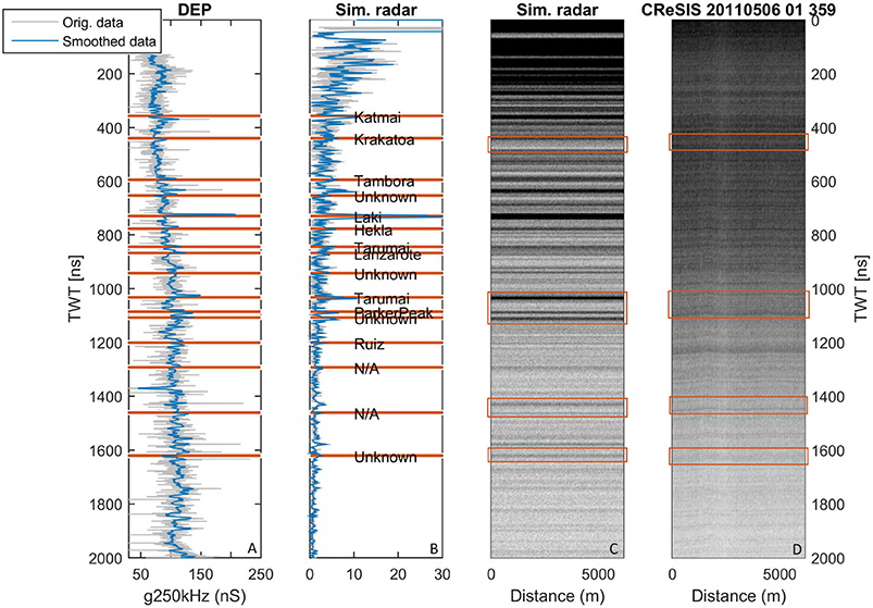
Figure 2. (A) DEP profile and (B) the corresponding simulated radar response (in arbitrary units). Gray lines are the original data, blue lines show the data smoothed with a moving average using a windowsize of 100 and 180 samples for (A,B), respectively. The orange lines indicate the volcanic horizons identified in the ice core and named in Sigl et al. (2013). (C) The simulated radar response as a Z-scope radargram, multiply plotting the same synthetic trace and with random noise added; (D) the CReSIS flight line 20110506_01_359 that were acquired a few kilometers from NEEM (colors indicate relative dB).

3.1. Electromagnetic Wave Propagation Model

The conversion of DEP data in the depth domain to radar data in the TWT–domain requires the ordinary relative permittivity of firn ε′(z), which determines radar wave speed V as a function of depth z as

$\begin{array}{ll}V(z)=c_0/\sqrt{\epsilon \prime (z)},& (1)\end{array}$

where c₀ is the speed of light in a vacuum. Permittivity of firn depends on the firn density and the permittivity of pure ice. The application of permittivity mixing formulae as well as the uncertainty in density data yield an effective uncertainty in the employed conversion from depth to TWT (Eisen et al., 2006). To reduce its impact, we employ radar-wave numerical modeling as established by Eisen et al. (2003) to optimize the uncertainty in the final conversion by matching synthetic radar signatures with the ones recorded by the radar data in the field. This can be considered as a calibration of the depth-TWT conversion.

Missing values of density and conductivity were linearly interpolated and the combined series resampled at a 5 mm sample interval. The DEP operations in the field did not provide sufficiently accurate calibration to determine absolute values of permittivity and conductivity to apply the complex-valued DECOMP equation (Eisen et al., 2006), which considers mixing of the real and imaginary parts of the permittivity in the two-phase firn system. The missing calibration of the DEP data is insignificant when obtaining reflections in synthetic radargrams, as these mainly depend on the relative changes in permittivity and conductivity. Ultimately, to obtain a reliable permittivity which determines the location of reflections at depth, we apply the real-valued Looyenga (1965) mixing model

$\begin{array}{ll}\epsilon \prime ={(\frac{\rho }{{\rho }_i}[\sqrt[3]{{\epsilon }_i^{\prime }}-1]+1)}^3,& (2)\end{array}$

using the available density records ρ with pure-ice values ρ_i = 917 kg m⁻³ and ${\epsilon }_i^{\prime }=3.15$. The latter value has commonly been derived from field measurements (e.g., Eisen et al., 2006) and confirmed by laboratory studies (Bohleber et al., 2012).

Conductivity and density serve as input data in the electromagnetic wave propagation model “emice,” a numerical representation of the Maxwell equations. We operated the model in one vertical dimension at 2 cm resolution, with conductivity accordingly averaged to that scale (cf., Eisen et al., 2006). In the upper part of the firn column, a number of synthetic radar reflections are generated by changes in the density data. As the footprint covered by the radar systems is more than an order of magnitude larger than the area covered by the firn core, considering the density at full resolution causes a higher level of ambiguities when connecting synthetic and real radar records. We therefore smoothed the density record with a running mean of 20 m. The smoothing preserved the average density but reduced the signal variability in the synthetic radar trace. The final synthetic trace is shown in Figures 2B,C.

3.2. Layer Matching

In order to assign an age to the observed layers in the CReSIS dataset, we construct a synthetic radargram using data from the NEEM11S1 shallow core as described above. This synthetic radargram is then compared to CReSIS data records that were acquired a few kilometers from NEEM. We calculated the correlation coefficient between the radargrams using offsets from −200 ns to 200 ns in increments of 5 ns. Correlation coefficients range from 0.42 to 0.6, with higher values (>0.54) for offsets larger than 10 ns. The best match, however, was found by manually comparing the two radargrams from observed and modeled data. Figure 2 shows the DEP profile, the simulated radargram and the CReSIS radargram. The matching volcanic signals are included in Table 1.

TABLE 1

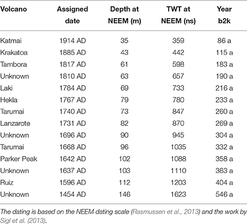
Table 1. Volcanoes used to construct the age-TWT relationship at NEEM.

We note that a strong signal in the DEP record (and consequently in the modeled data) is not necessarily reflected in the observed data as a distinct layer. For example, the Laki eruption of 1782–1784 is one of the five strongest DEP signals for the entire Holocene in the NEEM core (Sigl et al., 2013), but there is no obvious candidate for this single strong reflection in the observed radar data. This is likely because the radar layers represent the average of the power reflected by potentially several horizons. We therefore base our matching not only on the existence of a layer but also on layer sequences, i.e., distinctive patterns of layers, rather than using reflection magnitudes.

The best match between modeled and observed radar data is obtained by shifting the simulated radargram upwards by approximately 55 ns which corresponds to a few meters of firn. This offset could be explained by several causes. One is probably due to the uncertainty in reconstructing the density and thereby the TWT in the upper few meters, since good density measurements are missing here. Another reason for the offset is undulations in the observed layers caused by the presence of the camp site, and we see a slight dip downwards in layer depths close to NEEM. This was also observed during the 2015 ground-based radar campaign. Finally, the shallow core was drilled on a small snow mound made by several years of camp activities, and such an offset is therefore not surprising. Thus, the identification of distinct layer patterns rather than individual layers form the basis for the matching. One example of such a pattern match is the double peak at approx. ~1100 ns (where the first peak is the Parker Peak eruption, 1641–1643 at 102 m) and the single, strongly-reflecting layer above (from the Tarumai eruption, 1667–1668 at 96 m). The pattern with a doublet and a single layer above is also present in the CReSIS data.

The identification of the layers with volcanic horizons leads to an age–TWT relationship that we use to date the traced layers. We use ages published by Sigl et al. (2013) and in the cases where the volcanic event spans several years, we use the average age. Because we are only considering the top few hundred meters of firn, the change in TWT with age is linear, which is in agreement with the age–depth relationship constructed from the NEEM core (Rasmussen et al., 2013). Note that two of the layers in Figure 2 (annotated N/A in Figure 2B) do not match any identified volcanic horizons even though a strong reflection was visible in both the modeled and observed radar data. During the layer tracing, we picked the most strongly reflecting and easily identifiable layers, which in some cases were not the volcanic horizons themselves. The ages of the traced layers were therefore calculated from the age-TWT relationship, rather than directly dated from the ice-core record. An example of a traced radargram can be seen in the Supplementary Figure S2.

3.3. Firn Model

The propagation of radar waves in firn is highly dependent on the density of the firn column. Thus, in order to convert TWT to true depth, we need a firn densification model. Several different modeling approaches exist, but the most common approach is based on the theory set up by Herron and Langway (1980), that assumes an exponential increase of density with time. The Herron–Langway model can be described by

$\frac{\text{d}\rho }{\text{d}t}=\{\begin{array}{ll}{c}_0({\rho }_i-\rho ),\hfill & \rho \le {\rho }_c\hfill \\ c_1({\rho }_i-\rho ),\hfill & {\rho }_c<\rho <{\rho }_i\hfill & (3)\end{array}$

where ρ is the density as a function of time (and depth), ρ_i is the constant density of ice, ρ_i = 917 kg m⁻³, ρ_c is the threshold density of 550 kg m⁻³, and c₀, c₁ are compaction rate constants that depend on the SMB, surface density ρ_s and temperature. For a more complete introduction to firn models, we refer the reader to the original study by Herron and Langway (1980), or several new studies that have expanded on this model (e.g., Arthern et al., 2010; Ligtenberg et al., 2011; Simonsen et al., 2013).

Herron and Langway (1980) suggest values for the surface density and their compaction rate constants based on measurements of firn and ice cores from Greenland and Antarctica. To get a good estimate of ρ_s, c₀ and c₁ for our study area, we compare seven density records collected across central and northern Greenland. This comparison can be found in the Supplementary Table 1 and Supplementary Figure S1 along with full citation of the data (see also Bolzan and Strobel, 1994; Wilhelms, 1996; Schwager, 2000). The comparison clearly shows that the recommended parameter values in the Herron-Langway model overestimate the densification for all sites. We therefore fit an exponential function of the Herron-Langway type to the mean of the density records and obtain the best fitting values for ρ_s, c₀ and c₁. Equation (3) is then solved using a Crank-Nicolson finite-difference method (Crank and Nicolson, 1996). This density profile is used as a first guess in the inverse method (described below). The unknown precise values of the parameters c₀, c₁ and ρ_s are estimated by the inverse model.

3.4. Inverse Method

The depth of radar layers for a given (time-varying) accumulation rate can be approximated using a 1D flow model, where we assume that the layers thin with a constant thinning rate:

$\begin{array}{ll}w(z)=-\frac{a}{H}(H-z)& (4)\end{array}$

where w is vertical velocity, a is accumulation rate in meter ice equivalent, H is the local ice thickness and z is depth, also in meter ice equivalent. This flow model is coupled to the densification model to obtain true depths, which can then be converted to an age-TWT scale for a given accumulation rate and given density profile. If all variables were known: layer depth, layer age and density profile, we could immediately calculate the accumulation since the deposition of the layer, as that would simply equal the amount of snow above the layer. In this study, we know the age of the layers, while the depth is only known in the TWT domain, which depends on the wave speed and thus density, which in turn depends on the accumulation rate along with other parameters. Our problem is, in other words, underdetermined. The use of an inverse method together with a priori information is the most suitable way to obtain a reasonably accurate range of solutions to the problem.

All data are horizontally interpolated to a 5 km grid. For each data point, we use the depths and ages of the traced layers to infer centennially averaged accumulation rates for the last 700 years, and the three parameters of the Herron-Langway firn model, ρ_s, c₀, and c₁, along the flight lines. The inversion is performed using an iterative inverse method where the misfit between the observed and modeled layer depth is minimized using a gradient descent technique (cf., Waddington et al., 2007).

The misfit we seek to minimize consists of two terms. The first term is the data-model misfit, given by

$\begin{array}{ll}{J}_d={\displaystyle \sum {\left(\frac{t_d-t_m(p\{n\})}{{\sigma }_d}\right)}^2},& (5)\end{array}$

where the subscripts d and m indicate data and model respectively, σ is the standard deviation, t is layer depths in TWT, and p is the set of model parameters for n observations. The term J_d measures how well the solution of the forward model fits the traced layer depths converted to TWT t_d.

The second term is a set of regularization constraints on the model parameters, which are added to the cost function to prevent overfitting the data and to avoid unphysical model parameter values. For the three densification parameters, this term is estimated as the deviation from the expected value of the parameter by

$\begin{array}{ll}{J}_{reg}^{(1)}={{\displaystyle \sum \left(\frac{\left|c_i\right\{n\}-c_{ref}|}{{\sigma }_c}\right)}}^2.& (6)\end{array}$

For the accumulation parameters, the term measures the spatial consistency as the deviation of an accumulation rate from the surrounding accumulation rates, weighted according to the inverse distance r between the points, thus given as

$\begin{array}{ll}{J}_{reg}^{(2)}={{\displaystyle \sum _i\left(\frac{{\Sigma }_j{({\dot{b}}_i-{\dot{b}}_j)}^2}{\nu r_{i,j}}\right)}}^2,& (7)\end{array}$

where ḃ_i is the accumulation rate at point i, ḃ_j is the accumulation rate at point j, r_ij is the distance between them, and ν is a normalization constant based on the expected spatial variability of the data. We set ν = 2.5 × 10⁻⁴. The combined regularization constraint:

$\begin{array}{ll}{J}_{reg}=J_{reg}^{(1)}+J_{reg}^{(2)},& (8)\end{array}$

will tend to produce a smooth solution of the model parameters (Aster et al., 2013). If this regularization constraint were not included, we could have obtained a smaller data-model misfit but that would have led to unphysical values and/or unphysically large spatial variability for the densification parameters and accumulation rate parameters. We evaluate the optimal weight of the regularization constraints, determining the trade-off between data-model misfit and model “smoothness” by an L-curve analysis (Aster et al., 2013).

The L-curve is constructed by considering the total misfit J = J_d + ωJ_reg. Here, J_reg and the corresponding J_d is plotted against each other for different values of ω, showing how either contributes to the total misfit. The value of ω that is closest to where this curve bends is chosen as the optimal weight (e.g., Aster et al., 2013).

The Jacobian of the total misfit, J, is calculated by perturbing each model parameter in turn to obtain the corresponding change in the total misfit. The correction to the model parameters which should minimize this, Δp, is then obtained following the approach of Waddington et al. (2007) (see also Nielsen et al., 2015). To avoid potential overshooting of the minimum in the iteration process, the model parameters are updated by αΔp (Aster et al., 2013), where we use a value of α = 0.5. The decrease in misfit with increasing iteration number is shown in the Supplementary Figure S3.

3.5. Uncertainty Assignment

Several uncertainties are associated with the methods presented here. We first address the uncertainties pertaining to the matching of the radar layers with the ice-core record and the corresponding age determination. When modeling the radar response to the measured changes in permittivity and conductivity (see Section 3.1), we make several assumptions. We linearly interpolate missing values of density and conductivity (in the upper part of the core), the permittivity of pure ice is assumed to be ${\epsilon }_i^{\prime }=3.15$ and we smooth the density signal to a lower resolution to avoid high-frequency signals. The first leads to an unknown offset in the record, while the assumption of ${\epsilon }_i^{\prime }=3.15$ was found to cause shifts on the order of 5–10 ns compared to using a value of ${\epsilon }_i^{\prime }=3.20$ or ${\epsilon }_i^{\prime }=3.10$. The impact of smoothing the density signal is not likely to cause shifts in the radargram but might mask some layers.

The uncertainties mentioned above impact the forward modeling of radar signals, but a larger contributing factor of uncertainty is probably our manual tracing of radar layers. Although utmost care was taken to ensure that the same layer was followed between different flight tracks, as the flight lines enter low accumulation areas, seemingly bright and distinct layers may merge and become difficult to trace. Likewise, when the accumulation increases, some times a layer splits into two or more layers. When tracing layers, we consistently checked crossover points between different flight lines. Where discrepancies were identified, the layer tracing was rectified for consistency. Typically, the errors were 20 ns or less.

The assignment of ages to the layers is also associated with an error. The best match between the simulated radargram and the observed radargram, established by experienced radar data analysts, relies on their subjective decision. It is difficult to assign a specific error range to this uncertainty and the validity of the age assignment is discussed in more detail in sections below. In order to test the impact of erroneous age assignment to the layers, we perturb the assigned ages randomly by ±15 a and assess the resulting difference in accumulation rates. We also run the model with a different age-TWT relationship to investigate the impact of potential dating errors on the accumulation rate. The results of these tests will also be discussed in Section 5.1.

Based on the considerations above we assign an uncertainty of 50 ns to the observed layer depths, in order to ensure that we are not overfitting the layers. This uncertainty is used in Equation (5) when calculating the allowed misfit.

4. Results

The inversion scheme returns the average accumulation rates during the period 1311–2011 CE (Common Era) in averages of 100 a. The inversion was performed with five iterations and an uncertainty of 50 ns. The solution converged after a few iterations (see Supplementary Figure S3).

Figure 3 shows the average accumulation rates for the period 1311–2011 CE. We retrieve accumulation rates between 110 and 250 kg m⁻² a⁻¹, with a mean value of 187 kg m⁻² a⁻¹. The NEEM ice core site is situated between the 200 and 210 kg m⁻² a⁻¹ contours, while NGRIP is between the 170 and 180 kg m⁻² a⁻¹ contours. The uncertainty in the 700 a average is estimated to 6%, which translates to 10–12 kg m⁻² a⁻¹ at the two ice cores sites. See below for a full treatment of uncertainty estimation.

FIGURE 3

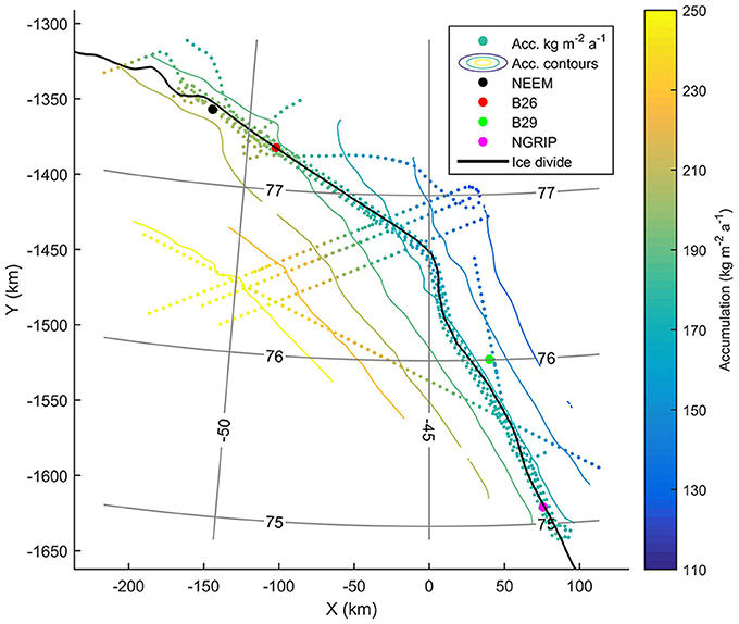
Figure 3. The average accumulation rate in kg m⁻² a⁻¹ for the period 1311–2011 CE (colored dots). Contour lines were constructed from interpolating the results to a smooth surface, where areas more than 30 km from observation points have been masked out. Ice core sites are as follows: NEEM (black), B26 (red), B29 (green) and NGRIP (pink). The present location of the ice divide is indicated with a black line.

Spatial variation in accumulation rates is clearly observed in Figure 3 and as expected, the accumulation rate increases as the elevation decreases. This manifests itself as a decrease in accumulation rates in the north-south direction. South of 76°N the ice divide lies approximately along the 170 kg m⁻² a⁻¹ contour. North of 76°N the ice divide bends into a lower accumulation area (between the 150 and 170 kg m⁻² a⁻¹ contours) but farther north it reenters a higher accumulation area. To further investigate this spatial variation, Figure 4 shows the results of the inversion on a section along the ice divide. The average accumulation rate (black line in Figure 4) decreases upstream from NEEM until approximately 170 km along the flight line, and after that the accumulation increases. From this point and upstream toward NGRIP, the accumulation rate is constant as the ice divide lies on an accumulation contour. We also recover a spatial gradient in the east-west direction: moving across the ice divide from west to east, there is a marked decrease in accumulation rates. The steep gradient in accumulation rates across the ice divide is evident from Figure 5, where the average accumulation rate for the period 1311–2011 CE drops from 270 kg m⁻² a⁻¹ to 120 kg m⁻² a⁻¹ over less than 200 km.

FIGURE 4

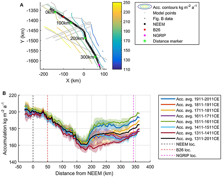
Figure 4. (A) Context map with the location of (B) shown as a black line and with accumulation contours corresponding to those shown in Figure 3. (B) Accumulation rates in kg m⁻² a⁻¹ during the period 1311–2011 CE along four flight lines following the ice divide. The thick lines represent the mean of the flight lines and the shading encompasses all values from the flight lines. The thick black line is the 1311–2011 CE average and the dashed lines mark the location closest to the ice-core sites.

FIGURE 5

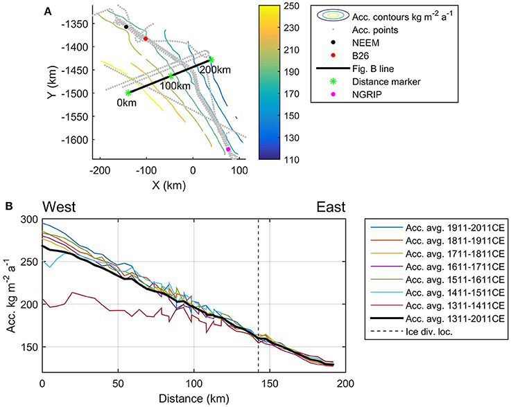
Figure 5. (A) Context map with the location of (B) shown as a black line and with accumulation contours corresponding to those shown in Figure 3. (B) Accumulation rates in kg m⁻² a⁻¹ during the period 1311–2011 CE following a flight line across the ice divide. The thick black line is the 1311–2011 CE average.

Finally, we consider the variation in the spatial pattern over time. Figure 4 shows the centennial accumulation rates vs. distance from NEEM. To ensure the robustness of the result, we combine all four flight lines along the ice divide to form the figure, and bin the accumulation rate results into bins of 5 km width, using the distance from NEEM as a distance scale. The thick colored lines show the mean of the centennial accumulation rate from each bin and the shading indicates the range of values in each bin (results from each flight line can be seen in the Supplementary Figures S5–S8). The shading pinches in the right-hand end of the plot because there is only one flight line represented in the last ~20 km. In Figure 4, a marked temporal variation is evident along the ice divide. The northern part of the section shows small variations in accumulation rate until approximately 170 km from NEEM. South of this point and to the NGRIP site the variation in accumulation is substantially larger, with the 1311–1411 CE average having the lowest accumulation rate and the 1911–2011 CE and 1511–1611 CE averages having the highest.

Figure 6 shows the accumulation rate anomalies for each 100 a period relative to the average accumulation rate for 1311–2011 CE (figures showing the absolute accumulation rates for the periods can be found in the Supplementary Figure S4). In the area around NEEM (all data points within 5 km of the camp) the accumulation rates for all periods are close to the 700 a average (within ±3%). This is in contrast to the southern half of the domain where anomalies occur. For example, the period 1511–1611 CE (Figure 6E) shows consistently high accumulation rates on both sides of the divide compared to the NEEM area, whereas the period 1711–1811 CE (Figure 6C) has higher accumulation in the southern part of the study area, but decreasing accumulation west of the ice divide. Most anomalies do not exceed ±10%.

FIGURE 6

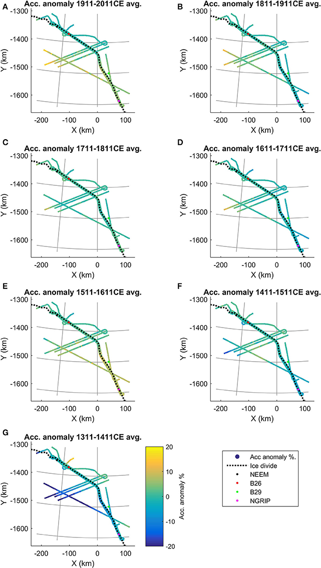
Figure 6. (A–G) Centennially averaged accumulation rates that have been normalized with respect to the accumulation rates for the period 1311–2011 CE. The gray grid lines indicate longitude–latitude. The periods shown are (A) 1311–1411 CE, (B) 1411–1511 CE, (C) 1511–1611 CE, (D) 1611–1711 CE, (E) 1711–1811 CE, (F) 1811–1911 CE, (G) 1911–2011 CE.

For the centennial averages the inverse scheme is not so well constrained, since each centennial average relies on fewer layers than for the 1311–2011 CE average. Particularly the end points are not as well resolved in these cases. The average accumulation pattern for the period 1911–2011 CE is especially uncertain since our youngest layer is 116 a old, and this accumulation pattern is therefore only constrained indirectly by the depth of the deeper layers.

5. Discussion

The NEEM and NGRIP ice-core sites are both located on the boundary between high and low accumulation areas in West and East Greenland. Our analysis indicates that the accumulation pattern at NEEM has been relatively stable for the period 1311–2011 CE. In contrast, we retrieve temporal variations in accumulation rate upstream from NEEM and around the NGRIP drill site. Below, we discuss the uncertainties that influence the confidence in our results and quantify the likely uncertainty range. We compare our results with accumulation rates estimated from ice-core records and outputs from regional climate models. Finally, we make a case for careful selection and interpretation of accumulation records from ice cores when elucidating a climate signal.

5.1. Uncertainties

The uncertainties in our study can be split into two groups: (i) uncertainties inherent in our applied method (i.e., the fact that we use a one-dimensional model that disregards horizontal ice flow, and the ability of the firn densification model to represent the density), and (ii) uncertainties introduced by errors in our procedure (for example, the errors associated with dating, matching, and tracing the layers).

We address the inherent uncertainties first. Using a one-dimensional model that only incorporates vertical advection (i.e., a local-layer approximation, Waddington et al., 2007; Nielsen et al., 2015) means that any horizontal transport of mass is not taken into account. West of the ice divide, a snow particle will travel through lower accumulation areas toward an area of high accumulation rates. In this case, our one-dimensional model underestimates the accumulation rate. The opposite is true east of the ice divide where particles travel from higher to lower accumulation areas. We therefore expect our findings to be a conservative estimate of spatial variations in accumulation rate. The application of a local layer approximation is justified partly because the study area is situated in a low ice-flow velocity region implying that the particles are not likely to have travelled far during the period of interest. Using balance velocities from the SeaRISE (Sea-level Response to Ice Sheet Evolution) project constructed by Johnson (2009), the estimated maximum distance that particles in our domain may have traveled in 700 a is 12 km. This is only a few grid points in our model resolution and not significant compared to the spatial variability of the expected accumulation pattern. By constructing the trajectories back in time, we can compare accumulation rates at the model grid with the accumulation rate at a point where the 700 a snow would have originated. In this way we find the largest discrepancy of 8%, but most points have a discrepancy of less than 5%. We therefore conclude that neglecting the horizontal advection is justified and is not significant for our results. This is in line with the findings of Nielsen et al. (2015). However, since the inverse scheme also imposes a degree of smoothness, it is likely that the accumulation rate gradient (e.g., across the divide) is more pronounced than our results suggest.

The densification model provides the input to convert depth to TWT. We assess this model by comparing the modeled density profile with two density profiles from shallow cores B26 and B29 (Figure 1), using the parameters obtained from the inverse method. The upper 20 m have a discrepancy between the observed density and the modeled density upwards of 40 kg m⁻³ (B26) and 60 kg m⁻³ (B29). Below 20 m the difference between model and observation is much smaller and does not exceed 20 kg m⁻³ for either core. When the modeled and observed density profiles are used in the depth–to–TWT conversion, the resulting difference is less than 10 ns for either core. This is well within our assigned data uncertainty of 50 ns. Thus, it seems unlikely that our densification model introduces significant uncertainties.

The second group of uncertainties is more difficult to assess. One uncertainty is introduced by the errors associated with matching, dating and tracing the radar layers. A mistake in dating would mean a shift in the accumulation rate for the whole traced layer dataset, while a mistake in the tracing (e.g., an erroneous jump from one layer to another) would impact the resulting accumulation pattern. We obtain a less than 3% difference between the NEEM accumulation record and our accumulation reconstruction (this is discussed below), and we are confident that the internal layers have been dated correctly. To test the impact of an incorrect layer dating further, we have run the model with an offset in the age-TWT relationship. The age-TWT relationship and the result of the test are included in the Supplementary Figures S9, S10. The offset causes the 1911–2011 CE accumulation rate to be substantially larger, and the corresponding 1311–2011 CE average accumulation rate is therefore increased. The overall pattern of decreasing accumulation rates until approximately 170 km from NEEM and then increasing accumulation rates persists. We also recover the same temporal variability of the accumulation rates (although not as clearly as in Figure 4), where the centennial averages seem to be more variable starting 170 km from NEEM. Thus, the variability is not strongly dependent on the dating of the layers, especially, the results based on the deeper (older) layers seem to be relatively robust.

It is also possible that errors were introduced in the process of tracing the layers. The main reason, however, why very few errors were introduced in the layer tracing, can be observed in Supplementary Figure S6. Here, there has been an error in one (or more) layers belonging to the 1711–1811 CE time period. The yellow line can be observed to suddenly decrease by ~10 kg m⁻² a⁻¹ at 260 km and then increase the same amount at 340 km. During the jumps the line fluctuates back and forth because all layers were traced with overlaps between neighboring flight lines, and the inverse method therefore received two conflicting TWT-values for the same locations This is the only place where we observe a jump in accumulation rate. To further test the impact of such an error, we have run the model while randomly assigning ±15 a (<2% offset) to the layer dating—corresponding to a jump in approximately 20 ns. This leads to discrepancies in accumulation rates upwards of 18% compared to ice core measurements. In other words, a small error in the age assignment (which is equivalent to tracing an incorrect layer) leads to discernible deterioration in the agreement between model results and observations. Therefore, we consider it likely that all errors in the layer tracing have been detected and corrected. Furthermore, the age–depth scale at NEEM forms the basis of our age assignment, and given the low misfit between the model results and the measurements at NEEM, it is unlikely that there have been significant errors when the layers were dated. Finally, we traced the layers starting at a high accumulation area and moving toward low accumulation areas. In this case, layers tend to pinch together thus picking the correct layer is less prone to errors than for areas where layers tend to split in two. Therefore, we argue that the spread in accumulation rates in Figure 4 reflects real changes in accumulation pattern in time. However, the exact value of the accumulation rate for the periods could be slightly higher or lower, and especially for the 1611–1711 CE period it is possible that there is a slow drift in our results leading to an overestimation in accumulation rate.

Figure 4 offers some insights into the uncertainty of our results. The figure shows a general trend of decreasing and then increasing accumulation over spatial scales of ≳10² km along the ice divide. In order to quantify the uncertainty, we consider any oscillation over a spatial scale smaller than ~10² km to be a result of the uncertainties in our method. Based on this consideration, we estimate that the centennially averaged accumulation rates have an uncertainty of ~12 kg m⁻² a⁻¹ and the 1311–2011 CE accumulation rate has an uncertainty of ~8 kg m⁻² a⁻¹. For the 1311–2011 CE accumulation rate, an uncertainty of ~8 kg m⁻² a⁻¹ corresponds at most to 6% of the reported accumulation rates. For the centennially averaged accumulation rates, an uncertainty of ~12 kg m⁻² a⁻¹ is translated into an 8% uncertainty based on the accumulation rates along the ice divide. As noted elsewhere, the centennially averaged accumulation rates are not well-behaved at end points in our domain and we therefore use the values along the ice divide to translate the ~12 kg m⁻² a⁻¹ uncertainty into a normalized uncertainty. Additionally, this kind of small scale variability in accumulation rate has been observed elsewhere in Greenland (Hawley et al., 2014). Thus, the oscillations might be correct and we therefore consider the normalized uncertainties mentioned above to be conservative estimates.

5.2. Comparison with Previous Records

Ice-core records, such as the deep ice cores NEEM and NGRIP (Andersen et al., 2006; Rasmussen et al., 2013) and the shallow cores B26 and B29 (Schwager, 2000; Weißbach et al., 2016), provide estimates of accumulation rates going back in time. We obtain a first insight into the spatial distribution of accumulation by comparing several cores with our model results. Additionally, we compare our findings with large-scale accumulation rates across Greenland estimated by regional climate models.

5.2.1. Spatial Distribution of Accumulation

Table 2 summarizes the comparisons between accumulation rates inferred from measurements of deep and shallow cores and our modeled results. With a few exceptions, differences between ice core measurements and model results fall within our stated uncertainty. For the B26 and B29 cores, the measurements only go back 500 a. Two studies have measured accumulation rates before; a study by Schwager (2000), and a more recent study by Weißbach et al. (2016). The latter constructed a new age–scale for the ice cores leading to slightly lower accumulation rates compared to the results by Schwager (2000). For the B26 core, the model results overestimate the accumulation rate compared to the measured rates. Potential reasons for this overestimation are discussed below. The difference between measured and modeled accumulation rates is smaller for the B29 core, where only the accumulation rates from Weißbach et al. (2016) fall outside our uncertainty range. This discrepancy is likely introduced by the difference in accumulation rates for the period 1911-2011 CE, where our results indicate anomalously high accumulation rates (174 ± 14 kg m⁻² a⁻¹), while the results from Weißbach et al. (2016) show low accumulation rates (138 kg m⁻² a⁻¹). This is also the period where our method is not well constrained. If instead the periods 1511-1911 CE are compared, the discrepancy decreases to 4% which is within our stated uncertainty.

TABLE 2

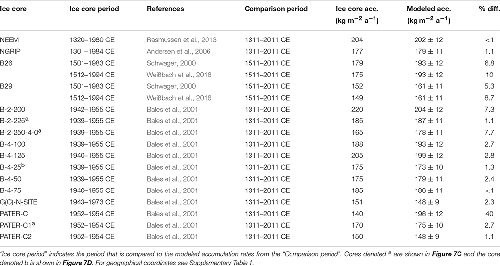
Table 2. Comparison between the modeled accumulation rates from this study and measured accumulation rates from ice and firn cores.

In Figures 7A,B we compare our findings with the output from two modeling studies by Ettema et al. (2009) and Burgess et al. (2010) respectively, which provide average SMB values for the period 1958–2007. Both studies use regional climate models (RCM) validated with in situ measurements from across the ice sheet. The models were run with a spatial resolution of 11 km (Ettema et al., 2009) and 24 km (Burgess et al., 2010) and the resulting accumulation rates are therefore smoother than our accumulation rates that are on a 5 km resolution. Note that we have regridded the RCM data to 5 km resolution for direct comparison with our results. In both studies, the accumulation pattern has a gradient across the ice divide, with contours approximately parallel to the ice divide. There is a notable difference in the value of the accumulation rate between the two studies. The accumulation rates at NEEM are 150 kg m⁻² a⁻¹ (Ettema et al., 2009) and 180 kg m⁻² a⁻¹ (Burgess et al., 2010), while at NGRIP the accumulation rates are 110 kg m⁻² a⁻¹ (Ettema et al., 2009) and 160 kg m⁻² a⁻¹ (Burgess et al., 2010). Our modeled accumulation rates display the same overall pattern but agree more strongly with the accumulation rates of Burgess et al. (2010). This is also evident from Figures 7C,D which show the accumulation rate along and across the ice divide. In contrast, the accumulation rates from Ettema et al. (2009) are on average 39 kg m⁻² a⁻¹ and 37 kg m⁻² a⁻¹ (along and across the ice divide, respectively) lower than our accumulation rates and those of Burgess et al. (2010). A study by Box et al. (2013) has shown that east of the ice divide, the model employed by Burgess et al. (2010) (Polar MM5) has the highest accumulation rates of the two RCMs. Interestingly, Vernon et al. (2013) found that Polar MM5 returns accumulation rates above observational values for areas with low accumulation rates. However, the Vernon et al. (2013) study does not include observations from our study region, so the discrepancy between observations and results might vary from region to region. For more in-depth discussions of SMB patterns from different RCMs, we refer the reader to the two studies referenced above. Here, we suggest that while the accumulation pattern presented in Ettema et al. (2009) is likely correct, the high–low accumulation boundary in Ettema et al. (2009) lies too far west, so that the accumulation rates at the ice divide are underestimated.

FIGURE 7

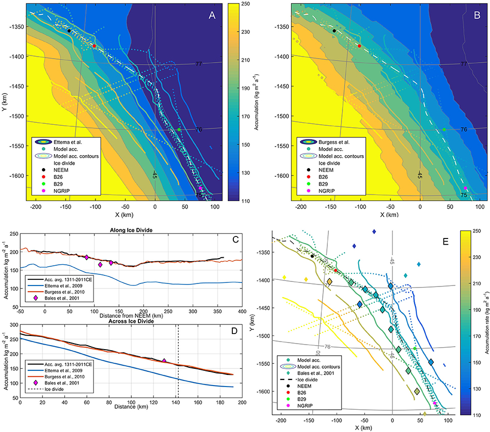
Figure 7. (A,B) Accumulation rates in kg m⁻² a⁻¹ (in colors) from (A) Ettema et al. (2009) and (B) Burgess et al. (2010) overlain with the accumulation rates from this study (colored dots and contour lines, see Figure 3). The ice divide location is indicated with a dashed white line and large circles mark the deep ice core sites NEEM and NGRIP, and shallow ice core sites B26 and B29. (C,D) Accumulation rates along and across the ice divide, respectively. The black lines correspond to the average 1311–2011 CE accumulation rate presented in Figures 4, 5. (E) Accumulation rate from the period 1311–2011 CE (colored dots and contours) and accumulation rates from shallow cores (Bales et al., 2001) as diamonds. The large diamonds outlined with black are within 30 km from our data points and have been used for comparison with our results (Table 2).

Our retrieved spatial pattern of accumulation can also be compared to results from studies of shallow ice-cores. In Figure 7E we show the results of Bales et al. (2001), who produced several short-term records of accumulation rates in our study area (see also Supplementary Table S1). The cores do not date further back than the 1930s but there is a clear agreement with our results (cf. Table 2). This agreement also indicates that the accumulation rates in the 1930s–1950s were similar to the 700 a average accumulation rate. The difference between the accumulation rates of Bales et al. (2001) and our results is 8% or less, with one exception: the PATER-C site located west of the ice divide at 76.72°N, −47.33°E (difference of 40%, see also Figure 7E). We do not have an immediate explanation for the large discrepancy at this site but it should be noted that the core in question only covers the period 1952–1954 CE. Thus, the discrepancy could either be an error in the dating of the core, or a localized accumulation phenomenon (in space and/or time).

5.2.2. Temporal Variation of Accumulation

We next compare the temporal variation of our modeled accumulation rates with the estimated temporal variation of accumulation rates from the ice cores (Figure 8). The model results from the last century are not discussed in the comparison because they are not well constrained due to the lack of layers in that age bracket. A comparison with the NEEM record (Figure 8A) shows minor discrepancies that are all well within our expected uncertainty. For the NGRIP record (Figure 8B), the difference between modeled accumulation rates and ice core measurements are larger than at NEEM. The largest difference occurs for the 1511–1611 CE period where the our model results are higher than the accumulation rates from the ice core. In contrast, the modeled accumulation rates are lower than the NGRIP record for the 1411–1511 CE and 1311–1411 CE period. With the exception of the 1511–1611 CE period, where modeled accumulation rates differ by 9% compared to the ice core measurements, the difference between the model results and the NGRIP record is less than 6%.

FIGURE 8

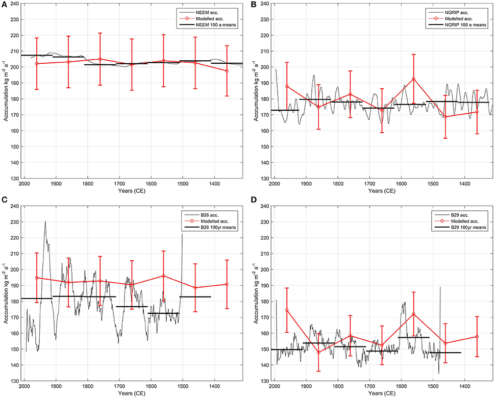
Figure 8. Comparison between accumulation rates from the inverse approach (red) with 8% errorbars and measured accumulation rates (black) with 100 a averages (thick black). The x–axis shows time in CE years with present day to the left. (A) The NEEM ice core (20 a resolution, Rasmussen et al., 2013). (B) NGRIP ice core (1 a resolution, smoothed over 20 a, Andersen et al., 2006), (C) B26 core (1 a resolution, smoothed over 20 a, Schwager, 2000) and (D) B29 core (1 a resolution, smoothed over 20 a, Schwager, 2000).

For the B26 core (Figure 8C), our centennially averaged accumulation rates all overestimate the accumulation rates compared to the ice core. The period 1511–1611 CE has the highest discrepancy (14%) while the other periods are within our uncertainty range of 8%. This is in contrast to the NEEM and NGRIP ice cores where the discrepancies between modeled and measured accumulation rates do not display a clear bias. Closer inspection of Figure 4B reveals that the model indicates a local accumulation minimum at this site, but the dip is probably obscured by the imposed smoothness of the inverse method and, the fact that upstream effects are not included in our one-dimensional model. This implies that the accumulation rates are overestimated by our model at this site. One factor contributing to the overestimated accumulation rates could be the location directly above a “unit of disrupted radiostratigraphy” identified by Panton and Karlsson (2015) (see Figure 4 in that study). These units of disrupted radiostratigraphy, although often originating from processes acting at the ice-bedrock interface, may cause disturbances all the way up to the ice surface. Thus, the depth of the layers may be influenced by processes other than accumulation, that are not included in our model. Similar to the results for the B26 core, the accumulation rates for the B29 core have the largest difference (9%) between model results and observations for the 1511–1611 CE period. All other periods have differences of less than 5%. For this core there is no clear bias in the modeled accumulation rates.

To summarize, our results agree well with ice core measurements. The period with the largest discrepancy is the 1511–1611 CE period. Considering that three out of four ice core sites indicate that our results for this period overestimate the accumulation rate, it is possible that an error was introduced either during our dating of (one of) the layers, or during our layer tracing. Results from the remaining periods (with the exception of the 1911–2011 CE period that we exclude) are robust and show consistent accumulation rate in the northern part of the model domain, and temporal variability in the southern part (e.g., Figure 4).

5.3. Representativeness of Ice-Core Accumulation Records

Our analysis indicates that in the area around NEEM the accumulation pattern has been stable for the period 1311–2011 CE. Changes in accumulation rates derived from this ice core can thus be reliably interpreted as changes in amount of precipitation on a regional scale in this part of Greenland. In contrast, we find changes in accumulation pattern starting approximately 170 km upstream from NEEM and around the NGRIP drill site. This implies that changes in accumulation rates from the NGRIP ice core might be influenced by, or even obscured by, changes in the accumulation pattern. Such changes can be triggered by a shift in the position of the ice divide. However, studies suggest that the relaxation time of the divide-position in response to changes in accumulation is 500–1000 years for the Greenland Ice Sheet (see Hindmarsh, 1996). We therefore consider it unlikely that the ice divide could have changed position to an extent that it affected the accumulation pattern. Instead, we attribute the changes in accumulation rates to migration of the accumulation pattern across the ice divide, and not ice divide displacement. In conclusion, care should be taken when interpreting variations in accumulation rate from the NGRIP ice core as an indicator of global or regional change in precipitation.

To summarize, there is overall agreement between our model results and measured accumulation rates from NEEM and NGRIP, and the shallow cores B26 and B29. Differences between our model and the observations for all periods (except for the period 1511–1611 CE) are less than 3% for NEEM, less than 6% for NGRIP, less than 8% for the B26 core, and less than 5% for B29 core. Although some uncertainties might have been introduced during the manual tracing of the layers, we find it likely that the variation in accumulation rate and thereby the implied shifts in accumulation pattern represent real climate events. This ultimately means that during the period 1311–2011 CE the NEEM ice core is more likely than the NGRIP ice core to have preserved a history of the past regional weather patterns that affected northern Greenland. Our assertion is based on the fact that the temporal accumulation signal is stable in the area around NEEM. In contrast, changes in accumulation rates deduced from the NGRIP core could reflect local shifts in accumulation patterns rather than a climate signal.

6. Conclusion

We used internal radar layers as input for a numerical model in order to retrieve accumulation rates. The crucial process of assigning correct ages to the layers was supported by the use of a model of electromagnetic wave propagation in ice, in conjunction with dielectric measurements and density data from the NEEM11S1 core. Using 16 dated and manually traced layers over an area encompassing the NEEM and NGRIP ice–core sites, and expanding 300 km across the ice divide, we retrieved accumulation rates in 100 a means for the period 1311–2011 CE. We used a gradient–descent inverse method that includes a 1D firn–densification model and solves for the best accumulation rates and densification parameters. Our modeled accumulation rates agree with spatially distributed model results from regional climate models. There is also good agreement between our centennial accumulation rate averages and measurements from the deep ice cores NEEM and NGRIP and the shallow cores B26 and B29. We find that while the NEEM ice-core site has stable accumulation rates during the study period, the NGRIP ice core is situated in a region that exhibits more temporal variability. The variability initiates approximately mid-way between NEEM and NGRIP. We interpret this variability as an indication of a locally varying accumulation pattern, specifically that the high–low accumulation boundary has migrated across the ice divide in the past. We consider it unlikely that the observed temporal variability is a result of ice divide migration, given the short time-scale in our study. Our study demonstrates the importance and value of acquiring radar data in the vicinity of ice core sites. It further underscores that mapping and interpretation of radar records may significantly contribute to reliable interpretation of accumulation rates derived from ice-core records on a regional scale, and provides insights into the weather patterns and thus the mass balance of polar ice sheets.

The traced layer depths and the centennial accumulation rates are available from the Centre for Ice and Climate website (http://www.iceandclimate.nbi.ku.dk/data/) or upon request from the corresponding author.

Author Contributions

NK and OE designed the study and wrote the manuscript. NK analyzed the radar data, traced the layers, constructed the firn model, did the layer matching and conducted the inverse model runs. OE constructed and calculated the synthetic radar trace. LN designed the inverse method. JF conducted the high resolution density measurements. SK did the DEP measurements and logged the NEEM11S1 core together with NK. JP and CL designed and operated the radar instrument and radar data processor. AW collected the 2015 radar data and contributed to the discussions. DD-J and FW secured the funding that made this study possible.

Funding

Funding for NK was provided by the European Research Council Advanced Grant no. 246815 WATERundertheICE. The Center for Ice and Climate is funded by the Danish National Research Foundation. Data and data products from CReSIS were generated with support from NSF grant ANT-0424589 and NASA grant NNX10AT68G, and NASA grant NNX10AT68G as a part of NASA Operation IceBridge.

Conflict of Interest Statement

The authors declare that the research was conducted in the absence of any commercial or financial relationships that could be construed as a potential conflict of interest.

Acknowledgments

This work initially started at the Karthaus summer school on Glaciers and Ice Sheets in 2013. We thank the long-term organizer Hans Oerlemans for his sustained efforts to bring together students and teaching scientists, enabling such spin-off results. The NEEM project is directed and organized by the Center of Ice and Climate at the Niels Bohr Institute and US NSF, Office of Polar Programs. It is supported by funding agencies and institutions in Belgium (FNRS-CFB and FWO), Canada (NRCan/GSC), China (CAS), Denmark (FIST), France (IPEV, CNRS/INSU, CEA, and ANR), Germany (AWI), Iceland (RannIs), Japan (NIPR), Korea (KOPRI), The Netherlands (NWO/ALW), Sweden (VR), Switzerland (SNF), United Kingdom (NERC) and the USA (US NSF, Office of Polar Programs). We acknowledge the use of data and data products from CReSIS. We acknowledge Prasad Gogineni for developing the concept of the airborne accumulation radar, Carl Leuschen for his work on the digital systems, and the CReSIS faculty, staff and students who contributed to the accumulation radar design, development, and deployment. The authors would like to thank J. MacGregor for use of his pickgui software. We thank our reviewers and editor, Felix Ng, for insightful and thorough comments that improved the manuscript.

Supplementary Material

The Supplementary Material for this article can be found online at: https://www.frontiersin.org/article/10.3389/feart.2016.00097/full#supplementary-material

References

Andersen, K. K., Ditlevsen, P. D., Rasmussen, S. O., Clausen, H. B., Vinther, B. M., Johnson, S. J., et al. (2006). Retrieving a common accumulation record from Greenland ice cores for the past 1800 years. J. Geophys. Res. 111:D15106. doi: 10.1029/2005JD006765

CrossRef Full Text | Google Scholar

Arthern, R. J., Vaughan, D. G., Rankin, A. M., Mulvaney, R., and Thomas, E. R. (2010). In situ measurements of Antarctic snow compaction compared with predictions of models. J. Geophys. Res. 115:F03011. doi: 10.1029/2009JF001306

CrossRef Full Text | Google Scholar

Aster, R. C., Borchers, B., and Thurber, C. H. (2013). Parameter Estimation and Inverse Problems. Cambridge, MA: Elsevier.

Bales, R. C., Guo, Q., Shen, D., McConnell, J. R., Du, G., Burkhart, J. F., et al. (2009). Annual accumulation for Greenland updated using ice core data developed during 2000–2006 and analysis of daily coastal meteorological data. J. Geophys. Res. 114:D06116. doi: 10.1029/2008JD011208

CrossRef Full Text | Google Scholar

Bales, R. C., McConnell, J. R., Mosley-Thompson, E., and Csatho, B. (2001). Accumulation over the Greenland ice sheet from historical and recent records. J. Geophys. Res. Atmos. 106, 33813–33825. doi: 10.1029/2001JD900153

CrossRef Full Text | Google Scholar

Bamber, J. L., Griggs, J. A., Hurkmans, R. T. W. L., Dowdeswell, J. A., Gogineni, S. P., I. Howat, J. M., et al. (2013). A new bed elevation dataset for Greenland. Cryosphere 7, 499–510. doi: 10.5194/tc-7-499-2013

CrossRef Full Text | Google Scholar

Bamber, J. L., Layberry, R. L., and Gogineni, S. P. (2001). A new ice thickness and bed data set for the Greenland ice sheet: 1. measurement, data reduction, and errors. J. Geophys. Res. Atmos. 106, 33773–33780. doi: 10.1029/2001JD900054

CrossRef Full Text | Google Scholar

Bohleber, P., Wagner, N., and Eisen, O. (2012). Permittivity of ice at radio frequencies: Part ii. artificial and natural polycrystalline ice. Cold Reg. Sci. Technol. 83,84, 13–19. doi: 10.1016/j.coldregions.2012.05.010

CrossRef Full Text | Google Scholar

Bolzan, J. F., and Strobel, M. (1994). Accumulation-rate variations around summit, Greenland. J. Glaciol. 40, 56–66. doi: 10.3198/1994JoG40-134-56-66

CrossRef Full Text | Google Scholar

Box, J. E., Cressie, N., Bromwich, D. H., Jung, J.-H., van den Broeke, M., van Angelen, J. H., et al. (2013). Greenland ice sheet mass balance reconstruction. Part I: net snow accumulation (1600962009). J. Clim. 26, 3919–3934. doi: 10.1175/JCLI-D-12-00373.1

CrossRef Full Text | Google Scholar

Burgess, E. W., Forster, R. R., Box, J. E., Mosley-Thompson, E., Bromwich, D. H., Bales, R. C., et al. (2010). A spatially calibrated model of annual accumulation rate on the Greenland Ice Sheet (1958-2007). J. Geophys. Res. 115:F02004. doi: 10.1029/2009JF001293

CrossRef Full Text | Google Scholar

Crank, J., and Nicolson, P. (1996). A practical method for numerical evaluation of solutions of partial differential equations of the heat-conduction type. Adv. Comput. Math. 6, 207–226. doi: 10.1007/BF02127704

CrossRef Full Text | Google Scholar

Dahl-Jensen, D., Albert, M. R., Aldahan, A., Azuma, N., Balslev-Clausen, D., Baumgartner, M., et al. (2013). Eemian interglacial reconstructed from a Greenland folded ice core. Nature 493, 489–494. doi: 10.1038/nature11789

PubMed Abstract | CrossRef Full Text | Google Scholar

Dahl-Jensen, D., Gundestrup, N. S., Keller, K., Johnsen, S. J., Gogineni, S. P., Allen, C. T., et al. (1997). A search in north Greenland for a new ice-core drill site. J. Glaciol. 43, 300–306.

Google Scholar

Eisen, O. (2008). Inference of velocity pattern from isochronous layers in firn, using an inverse method. J. Glaciol. 54, 613–630. doi: 10.3189/002214308786570818

CrossRef Full Text | Google Scholar

Eisen, O., Frezzotti, M., Genthon, C., van den Broeke, E., Dixon, D. A., Ekaykin, A., et al. (2008). Ground-based measurements of spatial and temporal variability of snow accumulation in East Antarctica. Rev. Geophys. 46:RG2001. doi: 10.1029/2006RG000218

CrossRef Full Text | Google Scholar

Eisen, O., Rack, W., Nixdorf, U., and Wilhelms, F. (2005). Characteristics of accumulation rate in the vicinity of the EPICA deep-drilling site in Dronning Maud Land, Antarctica. Ann. Glaciol. 41, 41–46. doi: 10.3189/172756405781813276

CrossRef Full Text | Google Scholar

Eisen, O., Wilhelms, F., Nixdorf, U., and Miller, H. (2003). Revealing the nature of radar reflections in ice: Dep-based fdtd forward modeling. Geophys. Res. Lett. 30:1218. doi: 10.1029/2002gl016403

CrossRef Full Text | Google Scholar

Eisen, O., Wilhelms, F., Steinhage, D., and Schwander, J. (2006). Instruments and Methods: Improved method to determine radio-echo sounding reflector depths from ice-core profiles of permittivity and conductivity. J. Glaciol. 52, 299–310. doi: 10.3189/172756506781828674

CrossRef Full Text | Google Scholar

Ettema, J., van den Broeke, M. R., van Meijgaard, E., van de Berg, W. J., Bamber, J. L., Box, J. E., et al. (2009). Higher surface mass balance of the Greenland ice sheet revealed by high-resolution climate modeling. Geophys. Res. Lett. 36:L12501. doi: 10.1029/2009GL038110

CrossRef Full Text | Google Scholar

Freitag, J., Kipfstuhl, S., and Laepple, T. (2013). Core-scale radioscopic imaging: a new method reveals density-calcium link in antarctic firn. J. Glaciol. 59, 1009–1014. doi: 10.3189/2013JoG13J028

CrossRef Full Text | Google Scholar

Frezzotti, M., Pourchet, M., Flora, O., Gandolfi, S., Gay, M., Urbini, S., et al. (2005). Spatial and temporal variability of snow accumulation in east Antarctica from traverse data. J. Glaciol. 51, 113–124. doi: 10.3189/172756505781829502

CrossRef Full Text | Google Scholar

Fujita, S., Holmlund, P., Andersson, I., Brown, I., Enomoto, H., Fujii, Y., et al. (2011). Spatial and temporal variability of snow accumulation rate on the east antarctic ice divide between dome fuji and EPICA DML. Cryosphere 5, 1057–1081. doi: 10.5194/tc-5-1057-2011

CrossRef Full Text | Google Scholar

Gfeller, G., Fischer, H., Bigler, M., Sch, S., Leuenberger, D., and Mini, O. (2014). Representativeness and seasonality of major ion records derived from neem firn cores. Cryosphere 8, 1855–1870. doi: 10.5194/tc-8-1855-2014

CrossRef Full Text | Google Scholar

Gogineni, P. (2012). Cresis Accumulation Radar Data. Lawrence: Digital Media.

Hanna, E., Huybrechts, P., Cappelen, J., Steffen, K., Bales, R. C., Burgess, E., et al. (2011). Greenland Ice Sheet surface mass balance 1870 to 2010 based on Twentieth Century Reanalysis, and links with global climate forcing. J. Geophys. Res. 116, 1–20. doi: 10.1029/2011JD016387

CrossRef Full Text | Google Scholar

Hawley, R. L., Courville, Z. R., Kehrl, L. M., Lutz, E. R., Osterberg, E. C., Overly, T. B., et al. (2014). Recent accumulation variability in northwest Greenland from ground-penetrating radar and shallow cores along the Greenland inland traverse. J. Glaciol. 60, 375–382. doi: 10.3189/2014JoG13J141

CrossRef Full Text | Google Scholar

Herron, M. M., and Langway, C. C. (1980). Firn densification: an empirical model. J. Glaciol. 25, 373–385.

Google Scholar

Hindmarsh, R. C. A. (1996). Stochastic perturbation of divide position. Ann. Glaciol. 23, 94–104.

Google Scholar

Johnson, J. (2009). Searise Master Data Set for Greenland. Missoula: University of Montana. Available online at: http://websrv.cs.umt.edu/isis/index.php/Present_Day_Greenland

Kanagaratnam, P., Gogineni, S. P., Ramasami, V., and Braaten, D. (2004). A wideband radar for high-resolution mapping of near-surface internal layers in glacial ice. IEEE Trans. Geosci. Remote Sens. 42, 483–490. doi: 10.1109/TGRS.2004.823451

CrossRef Full Text | Google Scholar

Koenig, L. S., Ivanoff, A., Alexander, P. M., MacGregor, J. A., Fettweis, X., Panzer, B., et al. (2016). Annual Greenland accumulation rates (2009–2012) from airborne snow radar. Cryosphere 10, 1739–1752. doi: 10.5194/tc-10-1739-2016

CrossRef Full Text | Google Scholar

Koutnik, M. R., Fudge, T. J., Conway, H., Waddington, E. D., Neumann, T. A., Cuffey, K. M., et al. (2016). Holocene accumulation and ice flow near the west antarctic ice sheet divide ice core site. J. Geophys. Res. Earth Surf. 121, 907–924. doi: 10.1002/2015jf003668

CrossRef Full Text | Google Scholar

Lenaerts, J. T. M., Brown, J., Broeke, M. R. v., Matsuoka, K., Drews, R., Callens, D., et al. (2014). High variability of climate and surface mass balance induced by Antarctic ice rises. J. Glaciol. 60, 1101–1110. doi: 10.3189/2014JoG14J040

CrossRef Full Text | Google Scholar

Lewis, C., Gogineni, S. P., Rodriguez-Morales, F., Panzer, B., Stumpf, T., and J. D. Paden, C. L. (2015). Airborne fine-resolution uhf radar: an approach to the study of englacial reflections, firn compaction and ice attenuation rates. J. Glaciol. 61, 89–100. doi: 10.3189/2015jog14j089

CrossRef Full Text | Google Scholar

Leysinger-Vieli, G., Hindmarsh, R., and Siegert, M. (2007). Three-dimensional flow influences on radar layer stratigraphy. Ann. Glaciol. 46, 22–28. doi: 10.3189/172756407782871729

CrossRef Full Text | Google Scholar

Ligtenberg, S. R. M., Helsen, M. M., and van den Broeke, M. R. (2011). An improved semi-empirical model for the densification of Antarctic firn. Cryosphere 5, 809–819. doi: 10.5194/tc-5-809-2011

CrossRef Full Text | Google Scholar

Looyenga, H. (1965). Dielectric constant of heterogeneous mixtures. Physica 31, 401–406. doi: 10.1016/0031-8914(65)90045-5

CrossRef Full Text | Google Scholar

MacGregor, J. A., Fahnestock, M. A., Catania, G. A., Paden, J. D., Gogineni, S. P., Young, S. K., et al. (2015). Radiostratigraphy and age structure of the Greenland Ice Sheet. J. Geophys. Res. Earth Surf. 120, 1–30. doi: 10.1002/2014JF003215

PubMed Abstract | CrossRef Full Text | Google Scholar

Nereson, N. A., Raymond, C. F., Jacobel, R. W., and Waddington, E. D. (2000). The accumulation pattern across siple dome, west antarctica, inferred from radar-detected internal layers. J. Glaciol. 46, 75–87. doi: 10.3189/172756500781833449

CrossRef Full Text | Google Scholar

Neumann, T. A., Conway, H., Price, S. F., Waddington, E. D., Catania, G. A., and Morse, D. L. (2008). Holocene accumulation and ice sheet dynamics in central west antarctica. J. Geophys. Res. 113:F02018. doi: 10.1029/2007JF000764

CrossRef Full Text | Google Scholar

Nielsen, L. T., Karlsson, N. B., and Hvidberg, C. S. (2015). Large-scale reconstruction of accumulation rates in northern Greenland from radar data. Ann. Glaciol. 56, 70–78. doi: 10.3189/2015AoG70A062

CrossRef Full Text | Google Scholar

North Greenland Ice Core Project members (2004). High-resolution record of Northern Hemisphere climate extending into the last interglacial period. Nature 431, 147–151. doi: 10.1038/nature02805

PubMed Abstract | CrossRef Full Text

Ohmura, A., and Reeh, N. (1991). New precipitation and accumulation maps for Greenland. J. Glaciol. 37, 140–148.

Google Scholar

Panton, C., and Karlsson, N. B. (2015). Automated mapping of near bed radio-echo layer disruptions in the Greenland Ice Sheet. Earth Planet. Sci. Lett. 432, 323–331. doi: 10.1016/j.epsl.2015.10.024

CrossRef Full Text | Google Scholar

Rasmussen, S. O., Abbott, P. M., Blunier, T., Bourne, A. J., Brook, E., Buchardt, S. L., Buizert, C., et al. (2013). A first chronology for the North Greenland Eemian Ice Drilling (NEEM) ice core. Climate Past 9, 2713–2730. doi: 10.5194/cp-9-2713-2013

CrossRef Full Text | Google Scholar

Richardson, C., and Holmlund, P. (1999). Spatial variability at shallow snow-layer depths in central Dronning Maud Land, East Antarctica. Ann. Glaciol. 29, 10–16. doi: 10.3189/172756499781820905

CrossRef Full Text | Google Scholar

Schwager, M. (2000). Ice core analysis on the spatial and temporal variability of temperature and precipitation during the late holocene in north Greenland. Rep. Polar Res. 362, 1–136. doi: 10.2312/BzP_0362_2000

CrossRef Full Text

Sigl, M., McConnell, J. R., Layman, L., Maselli, O., McGwire, K., Pasteris, D., et al. (2013). A new bipolar ice core record of volcanism from WAIS Divide and NEEM and implications for climate forcing of the last 2000 years. J. Geophys. Res. 118, 1151–1169. doi: 10.1029/2012JD018603

CrossRef Full Text | Google Scholar

Simonsen, S. S., Stenseng, L., Adalgeirsdóttir, G., Fausto, R. S., Hvidberg, C. S., and Lucas-Picher, P. (2013). Assessing a multilayered dynamic firn-compaction model for Greenland with asiras radar measurements. J. Glaciol. 59, 545–558. doi: 10.3189/2013JoG12J158

CrossRef Full Text | Google Scholar

Steinhage, D., Eisen, O., and Clausen, H. B. (2004). Regional and temporal variation of accumulation around North-GRIP derived from ground based ice-penetrating radar. Ann. Glaciol. 42, i326–i330. doi: 10.3189/172756405781812574

CrossRef Full Text

Vernon, C. L., Bamber, J. L., Box, J. E., Broeke, M. R. V. D., Fettweis, X., Hanna, E., et al. (2013). Surface mass balance model intercomparison for the Greenland ice sheet. Cryosphere 7, 599–614. doi: 10.5194/tc-7-599-2013

CrossRef Full Text | Google Scholar

Waddington, E. D., Neumann, T. A., Koutnik, M. R., Marshall, H.-P., and Morse, D. L. (2007). Inference of accumulation-rate patterns from deep layers in glaciers and ice sheets. J. Glaciol. 53, 694–712. doi: 10.3189/002214307784409351

CrossRef Full Text | Google Scholar

Weißbach, S., Wegner, A., Opel, T., Oerter, H., Vinther, B. M., and Kipfstuhl, S. (2016). Spatial and temporal oxygen isotope variability in northern Greenland – implications for a new climate record over the past millennium. Clim Past 12, 171–188. doi: 10.5194/cp-12-171-2016

CrossRef Full Text | Google Scholar

Wilhelms, F. (1996). Measuring the conductivity and density of ice cores. Rep. Polar Res. 191. Available online at: http://epic.awi.de/3394/