Evaluation of the Use of Moist Potential Vorticity and Moist Potential Vorticity Vector in Describing Annual Cycles of Rainfall over Different Regions in Tanzania

Introduction

The general circulation models (GCMs) represent the most satisfactory approach for predicting climate change (IPCC, 2013). They describe the relevant physical processes in the atmosphere, hydrosphere, and cryosphere that make up the climate system. However, GCMs have coarse spatial resolutions and cannot resolve small scale features such as orography, and land use land change that characterize the climate of many regions in the world. This makes their climate simulations of limited use in impact studies of climate change on for instance biodiversity, ecosystem services, agricultural systems, species distributions, conservation planning, and other landscape related matters (Villegas and Jarvis, 2010; Daniels et al., 2012; Tumbo et al., 2012; Xiaoduo et al., 2012; Hassan et al., 2013; Vigaud et al., 2013). These types of impact studies require climate information with much finer spatial resolution.

Downscaling of GCMs outputs is a widely applicable technique for obtaining high resolution climate information that takes into account regional patterns and valuable local knowledge. It is defined as a process of making a link between the state of some atmospheric variable representing a large space (henceforth referred to as the “large scale”) and the state of some atmospheric variable representing a smaller space (henceforth referred to as the “small scale”) (Benestad et al., 2007).

There are two broad categories of downscaling techniques (Hewitson and Crane, 1996). The first category is the dynamical downscaling. This is based on nesting a high resolution regional climate model (RCM) within GCM and drives it using boundary condition from GCM (Danis et al., 2002). The second category is statistical downscaling. This is based on establishing statistical links between large scale atmospheric variables (predictors) and local scale atmospheric variables (predictands).

Dynamical downscaling technique has been extensively used to provide high resolution climate simulation over different regions (Danis et al., 2002; Jones et al., 2004; Roux, 2009; Wilby and Fowler, 2011; Xiaoduo et al., 2012). However, this technique suffers to reproduce the spatial and temporal distributions of climate variables with strong spatial and temporal variability such as rainfall. This is due to fact that the contemporary numerical grids of the RCMs are still too coarse to represent all drivers of rainfall at local scales, circulation patterns, small scale topography, thunderstorms and cloud micro-physics processes (Goosse et al., 2010; Wilby and Fowler, 2011).

Statistical downscaling can be employed to better or adjust the output from RCMs (Benestad et al., 2007). The statistical downscaling techniques require the selection of realistic predictors that are relevant to the predictands. Several researchers (Zorita and Von storch, 1999; Chen et al., 2010; Villegas and Jarvis, 2010; Hassan et al., 2013; Vigaud et al., 2013; Muchuru et al., 2014) have used predictors such as, sea level pressure, Sea Surface Temperature (SST), geo-potential height, wind fields, relative humidity, or temperature variables in statistical downscaling to develop predictors-predictands transfer functions.

However, some of the predictors that are used for statistical downscaling are debated in literatures. For instance, the sea surface temperatures (SSTs), which partly depends on the ocean dynamics, is not represented well in ocean models (Benestad et al., 2007). The spatial resolution of these models tends to be too coarse to describe the ocean currents which are important influences on the SSTs. Fung et al. (2011) argued that circulation predictors alone are unlikely to capture precipitation mechanisms linked to thermodynamics and vapor contents. Wilby and Wigley (2000) suggest that atmospheric moisture must be considered as predictors as well as atmospheric circulations. Charles et al. (1999) suggest that inclusion of moisture variables as predictors can lead to convergence between statistical and dynamical downscaling approaches.

Therefore there is no consensus in literature about the most appropriate predictor to be used in statistical downscaling (Fung et al., 2011). In this study we explore the use of MPV to describe annual cycles of rainfall over different regions of Tanzania to see if it can be used as a predictor for downscaling climate change projections. The same task is performed using the moist potential vorticity vector $(\overrightarrow{MPVV})$ which is a modified version of convective vorticity vector ($\overrightarrow{CVV}$) defined by Gao et al. (2004b).

Background Information on Potential Vorticity

The concept of Potential Vorticity (PV) has long history in the study of fluid dynamics. It has been used in meteorology and oceanography for many years back (see Bjerknes, 1898a; Rossby, 1939; Ertel, 1942). This concept has many applications in meteorology, oceanography and aerodynamics (Hoskins et al., 1985). It is mentioned in Hoskins et al. (1985) that “PV can be used to understand the dynamics and thermal conditions of atmospheric flow to the lower limit to the fineness of the structures that may occur, all the way down to the length scales at which molecular diffusion acts.” Many important synoptic scale processes can be understood within the framework of PV. Recently McIntyre (2015) indicated that PV can explain the balanced flows and basic dynamical processes of large scale features such as breaking and propagation of Rossby-wave and its many consequences in the Earth's atmosphere. PV can describe global-scale teleconnections, anti-frictional phenomena such as jet stream self-sharpening, and the genesis of cyclones, anticyclones and storm tracks. PV is conservative and is subject to invertibility principle (Hoskins et al., 1985). The conservative and invertibility properties of PV form the bases of understanding many important atmospheric flow processes.

Ertel (1942) definition of PV see Schubert et al. (2004) is

$\begin{array}{cc}PV(\theta )={\rho }^{-1}{\zeta }_a·\nabla (\theta ),& (1)\end{array}$

where ρ is density of air, ζ_a is absolute vorticity and ∇(θ) is three dimensional gradient of the potential temperature. This definition emerged from fundamental concepts on circulation and vorticity that have been laid in the works of Bjerknes (1898a,b) and Rossby (1936, 1938, 1940).

Equation (1) is often used to study the thermodynamic properties of the atmosphere (Hoskins and Sardeshmukh, 1987; Stoelinga, 1996; Hoskins, 1997) while it is based only on dry-air potential temperature θ. In moist atmosphere, Equation (1) is not conserved when latent heat release is taken into account (Cao and Cho, 1995; Mofor and Lu, 2008). To avoid this drawback, Bennetts and Hoskins (1979) defined a moist potential vorticity (MPV) by replacing dry-air potential temperature θ with wet bulb potential temperature θ_w as;

$\begin{array}{cc}MPV({\theta }_w)={\rho }^{-1}{\zeta }_a·\nabla ({\theta }_w).& (2)\end{array}$

However, θ_w in Equation (2) cannot fulfill the demand to verify at the same time the conservative property of the moist air and invertibility principle (Marquet, 2014).

Therefore neither Equation (1) nor Equation (2) can be used to study non-uniform saturated atmospheric flow and fulfill the demand to verify, at the same time, a moist and dry air conservative property and an invertibility principle. To overcome this drawback Gao et al. (2004a) defined a new Generalized Moist Potential Vorticity (GMPV) by replacing θ with a Generalized Potential Temperature GMPV(θ*) (GPT) as;

$\begin{array}{cc}GMPV({\theta }^{\ast })={\rho }^{-1}{\zeta }_a·\nabla ({\theta }^{\ast }),& (3)\end{array}$

where θ is defined as;

$\begin{array}{cc}{\theta }^{\ast }(T,p,q)=\theta exp\left(\frac{L{q}_s}{C_{p}T}{\left(\frac{q}{q_s}\right)}^k\right),& (4)\end{array}$

where q and q_s are specific humidity and saturated specific humidity respectively, ${\left(\frac{q}{q_s}\right)}^k$ is a condensation probability function. In case of absolutely dry atmosphere where q = 0, Equation (4) reduces to dry potential temperature θ*(T, p, q) = θ while in completely saturated atmosphere where q = q_s it reduces to equivalent potential temperature ${\theta }^{*}(T,p,q)={\theta }_e=\theta exp\left(\frac{L{q}_s}{C_{p}T}\right)$. In realistic atmosphere which is non-uniformly saturated, the introduction of condensation probability function fixes the discontinuity of latent heat term due to the impact of water phase changes in the thermodynamic equation. Therefore a smooth transition from completely dry atmosphere and saturated atmosphere is achieved through the change of specific humidity from q to q_s. Equation (4) has been used in computation of MPV (Gao et al., 2004a; Mofor and Lu, 2008; Liang et al., 2010; Yang et al., 2014), and found that the solenoidal term does not cancel out in the MPV tendency equation in moist and dry atmosphere. However, Gao et al. (2004a) noted some limitations of applicability of the condensation density function in regions of no condensation or lower relative humidity conditions.

Recently Marquet (2014) defined a new MPV using the specific entropy formulation expressed in terms of moist-air entropy potential temperature (θ_s) as;

$\begin{array}{cc}MPV({\theta }_s)=\frac{1}{\rho }{\zeta }_a·\nabla ({\theta }_s),& (5)\end{array}$

where θ_s is defined in Marquet (2011) as;

$\begin{array}{cc}{\theta }_s\equiv {({\theta }_s)}_1{\left(\frac{T}{T_r}\right)}^{⋋q_t}{\left(\frac{p}{p_r}\right)}^{-k\delta q_t}{\left(\frac{r_r}{r_v}\right)}^{\gamma q_t}\frac{{(1+\eta r_v)}^{k(1+\delta q_t)}}{{(1+\eta r_r)}^{k\delta q_t}},& (6)\end{array}$

$\begin{array}{cc}{({\theta }_s)}_1=\theta exp({\Lambda }_r{q}_t)exp\left(-\frac{L_v{q}_l+L_s{q}_i}{c_{pd}T}\right),& (7)\end{array}$

where ${\Lambda }_r=\frac{\left(s_v^0-s_d^0\right)}{c_{pd}}\approx 5.87$ is a key quantity. It is mentioned in Marquet (2011) that Λ_r depends on the standard entropies of water vapor and dry air ($s_v^0$ and $s_d^0$). It is also mentioned that (θ_s)₁ is a good approximation of θ_s. For detailed derivation of θ_s the reader may consult Marquet (2011, 2014). The main advantage of θ_s, is that it represent exactly the moist air entropy, it is valid for a general mixing of dry air, water vapor and all possible condensed water species. It is mentioned in Marquet (2014) that “θ_s verifies the same conservative properties as the moist entropy, even for varying dry air or total water content”. The moist formulation for θ_s is valid for a general mixing of dry air, water vapor, and all possible condensed water species (Marquet, 2011). In this paper, we compute Marquet (2014)'s MPV formulation and explore its usefulness as a predictor of the annual cycles of rainfall over different regions of Tanzania.

We also suggest a modification of the convective vorticity vector ($\overrightarrow{CVV}$) proposed by Gao et al. (2004b) by replacing the equivalent potential temperature θ_e with conservative moist-air entropy potential temperature (θ_s) to form moist potential vorticity vector ($\overrightarrow{MPVV}$). This vector is also evaluated as a predictor of annual cycles of rainfall over different regions in Tanzania. We argue that the results from the scalar product of absolute vorticity and gradient of temperature may not explain all atmospheric dynamics over the tropics that contribute to formation and distribution of rainfall events. This is due to (1) the Coriolis parameter that contributes for many dynamical processes in mid and extra tropical regions is very small over the tropics and is zero over the equator. Therefore equatorial flows, especially two dimensional equatorial flows, may not be explained by any version of MPV as Gao et al. (2004b) argued. (2) The vertical gradient of temperature over the tropics is small due to strong convective mixing processes. The scalar MPV derived from dot product of absolute vorticity and gradient of temperature may not be accurate enough to explain convective processes associated with rainfall events over tropics.

Data and Analysis

Study Area

Tanzania (Figure 1) is located in East Africa between longitudes 29° to 41°E and latitudes 1° and 12°S. The country has an area of 945,000 km² of which 884,000 km² is land mass and 61,000 km² is lakes, rivers and seashore. Tanzania has complex topography that is very heterogeneous. The height of the topography ranges from sea level in the East to 1600 m in the West. In the northeastern highlands is the highest mountain in Africa: Mt Kilimanjaro with an altitude of 5895 m, while in the north is the largest lake in Africa: Lake Victoria. In the south is Lake Nyasa and the Ruvuma river, and in the west is the deepest lake in Africa: Lake Tanganyika. Much of the country lies above 1000 m altitude with many areas over central and northern regions above 1500 m.

FIGURE 1

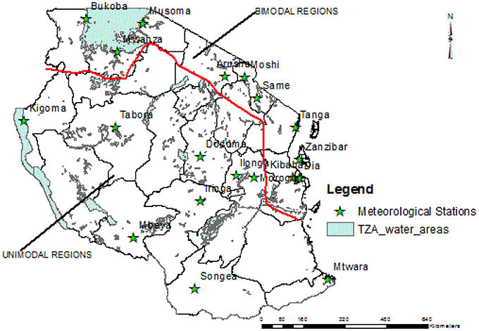
Figure 1. Map of Tanzania showing the location of meteorological stations in Unimodal and Bimodal regions separated by the red line.

The climate over Tanzania is mainly controlled by the movement of the Inter-Tropical-Convergence-Zone (ITCZ). However, seasonal interactions within the ITCZ, perturbations in global climate circulation and changes in local circulation systems which are influenced by complex topographical features all contribute to high local climate variability. The seasonal rainfall is modulated by changes in the global sea surface temperatures (SSTs) especially over the equatorial Pacific and Indian Oceans (Black et al., 2003; Black, 2005; Anyah and Semazzi, 2007).

Tanzania is characterized by two rainfall seasons, namely March-April-May (MAM) and October-November-December (OND). These seasons are mainly driven by the migration of the ITCZ, which lags behind the overhead sun by 3–4 weeks over the region (Luhunga et al., 2016). The ITCZ migrates toward southern regions of Tanzania in October-December, reaching southern parts of the country in January-February and reverses northwards in March, April and May (Timiza, 2011). Due to this movement, some areas experience single and double passages of the ITCZ (Luhunga et al., 2016). Regions with a single passage are known as unimodal areas (see Figure 1) and include the southern, southwestern, central and western parts of the country which receive rainfall from October through to April or May (Timiza, 2011). Areas that experience a double passage are known as bimodal areas, and include north, northern coast, northeastern highlands, the Lake Victoria basin and the islands of Zanzibar (Unguja and Pemba). These regions receive two distinct rainfall seasons; the long rain season (known as Masika in Swahili) which starts in March and continues through May (MAM) and the short rainfall season (Vuli in Swahili) which starts in October and continues through December (OND) (Agrawala et al., 2003).

The amount of seasonal rainfall varies significantly in space and time, with higher variation observed during the Vuli season than in Masika. The rainfall falling in these seasons usually ranges from 50 to 200 mm per month but varies greatly between regions and can be as much as 300 mm per month in wettest regions and seasons (McSweeney et al., 2010). Higher amounts of seasonal rainfall are recorded over the southwestern and northeastern highlands, while central Tanzania is semi-arid, receiving seasonal rainfall of less than 50 mm per month. Annual average rainfall over Tanzania ranges from 534 to 1837 mm.

Model Data

Rossby center has produced and made available a very large number of climate simulation that are included in the Coordinated Regional Downscaling Experiment (CORDEX). Rossby Centre Atmospheric (RCA) model is driven by several general circulation models (GCMs) and ERA-Interim global reanalysis datasets (Strandberg et al., 2014). In this study daily data of air temperature, specific humidity, zonal and meridional components of the wind at 850 and 600 hPa from numerical output generated by the Rossby Center regional climate model version four (RCA4) forced by CCCma-CanESM2 (GCM) are used for computation of MPV and $\overrightarrow{MPVV}$ at 700 hPa. RCA4 has high space resolution of 0.4⁰ by 0.4⁰ corresponding to 50 km by 50 km and has 10 vertical levels (standard pressure levels).

The land surface characteristics used to initialize Soil-Vegetation-Atmosphere Transfer schemes (SVTs) in RCA4 come from a new global physiography data bases ECOCLIMAP for vegetation, lake depth and soil carbon density, and Gtopo30 for orography. The near surface diagnostic quantities: temperature, specific humidity and wind speed are solved using new version of Turbulence Kinetic Energy (TKE) scheme (Strandberg et al., 2014). This scheme combines TKE based on local stability measurement (using Richardson number) and the non-local parcel method. Convection scheme in RCA4 is based on Bechtold-KF (Strandberg et al., 2014). In this scheme the triggering function forcing for convection is the large scale vertical velocity, closure assumption and cloud top is based on CAPE closure (Bechtold et al., 2001).

Observation Data

Monthly observation rainfall data from 22 synoptic meteorological stations over the period of 1976–2001 are obtained from the Tanzania Meteorological Agency (TMA). These data are quality controlled to remove the inhomogeneity and gaps by using the HOMER software package. For detailed descriptions of methodology used for homogeneity tests the reader may consult Luhunga et al. (2014).

Analysis

Marquet (2014)'s MPV

For simplification of the analysis Equation (5) can be re-written into three terms under hydrostatic balance as;

$\begin{array}{cc}MPV({\theta }_s)=-g\left(-\frac{\partial v}{\partial p}\frac{\partial {\theta }_s}{\partial x}+\frac{\partial u}{\partial p}\frac{\partial {\theta }_s}{\partial y}+(\zeta +f)\frac{\partial {\theta }_s}{\partial p}\right),& (8)\end{array}$

$\begin{array}{cc}\text{first}\text{term}=MP{V}_z=-g(\zeta +f)\frac{\partial {\theta }_s}{\partial p},& (9)\end{array}$

$\begin{array}{cc}\text{second}\text{term}=MP{V}_x=g\frac{\partial v}{\partial p}\frac{\partial {\theta }_s}{\partial x},& (10)\end{array}$

$\begin{array}{cc}\text{third}\text{term}=MP{V}_y=-g\frac{\partial u}{\partial p}\frac{\partial {\theta }_s}{\partial y}.& (11)\end{array}$

The Moist Potential Vorticity Vector ($\overrightarrow{MPVV}$)

Gao et al. (2004b) defined convective vorticity vector as;

$\begin{array}{cc}\overrightarrow{CVV}=\frac{{\zeta }_a\times \nabla {\theta }_e}{\rho }.& (12)\end{array}$

We modify Equation (12) by replacing θ_e with θ_s to form $\overrightarrow{MPVV}$ as;

$\begin{array}{cc}\overrightarrow{MPVV}({\theta }_s)=\frac{{\zeta }_a\times \nabla {\theta }_s}{\rho },& (13)\end{array}$

Equation (13) can be re-written into component form as;

$\begin{array}{cc}\begin{array}{l}\begin{array}{ccc}\overrightarrow{MPVV}({\theta }_s)& =& \frac{1}{\rho }\left(\begin{array}{c}\begin{array}{c}-\frac{\partial v}{\partial z}\\ \frac{\partial u}{\partial z}\end{array}\\ (\zeta +f)\end{array}\right) \times \left(\begin{array}{c}\frac{\partial {\theta }_s}{\partial x}\\ \frac{\partial {\theta }_s}{\partial y}\\ \frac{\partial {\theta }_s}{\partial z}\end{array}\right)\end{array}\\ \begin{array}{cc}=& \frac{1}{\rho }\left(\begin{array}{c}\frac{\partial u}{\partial z}\frac{\partial {\theta }_s}{\partial z} - (\zeta +f)\frac{\partial {\theta }_s}{\partial y}\\ \frac{\partial v}{\partial z}\frac{\partial {\theta }_s}{\partial z}+(\zeta +f)\frac{\partial {\theta }_s}{\partial x}\\ -\frac{\partial v}{\partial z}\frac{\partial {\theta }_s}{\partial y}-\frac{\partial u}{\partial z}\frac{\partial {\theta }_s}{\partial x}\end{array}\right)=\left(\begin{array}{c}{\overrightarrow{MPVV}}_x\\ {\overrightarrow{MPVV}}_y\\ {\overrightarrow{MPVV}}_z\end{array}\right)\end{array}\end{array}& \left(14\right)\end{array}$

where ρ is density which is defined as

$\begin{array}{cc}\rho =\frac{p}{{\theta }_v(p,T,q_v)R_d}{\left(\frac{p_0}{p}\right)}^k,& (15)\end{array}$

where p is atmospheric pressure (in Pa) at different level, p₀ is atmospheric pressure at reference level, θ_v(p, T, q_v) is virtual potential temperature, R_d is specific gas constant for dry air and $k=\frac{R_d}{c_p}$, c_p is specific heat capacity at constant pressure. The absolute vorticity ζ_a is the is defined as;

$\begin{array}{cc}{\zeta }_a=-\frac{\partial v}{\partial z}\overrightarrow{i}+\frac{\partial u}{\partial z}\overrightarrow{j}+\left(\zeta +f\right)\overrightarrow{k},& (16)\end{array}$

where ζ is the relative vorticity defined as $\zeta =\left(\frac{\partial v}{\partial x}-\frac{\partial u}{\partial y}\right)\vec{k}+\frac{u}{a}tan\left(\phi \right)$, where a is the radius of the earth and φ is the latitude, f is the coriolis parameter defined as f = 2Ωsin(φ).

Considering the hydrostatic equilibrium ∂/∂z = −ρg∂/∂p, Equation (14) can be re-written as;

$\begin{array}{cc}\text{first}\text{component}{\overrightarrow{MPVV}}_{\text{x}}\text{=}\rho g^2\frac{\partial u}{\partial p}\frac{\partial {\theta }_s}{\partial p}-\frac{(\zeta +f)}{\rho }\frac{\partial {\theta }_s}{\partial y},& (17)\end{array}$

$\begin{array}{cc}\text{second}\text{component}{\overrightarrow{MPVV}}_{\text{y}}=\rho g^{\text{2}}\frac{\partial \text{v}}{\partial p}\frac{\partial {\theta }_s}{\partial p}+\frac{\left(\zeta +f\right)}{\rho }\frac{\partial {\theta }_s}{\partial x},& (18)\end{array}$

$\begin{array}{cc}\text{third}\text{component}{\overrightarrow{MPVV}}_{\text{z}}\text{=}g\left(\frac{\partial v}{\partial p}\frac{\partial {\theta }_s}{\partial y}+\frac{\partial u}{\partial p}\frac{\partial {\theta }_s}{\partial x}\right),& (19)\end{array}$

$\begin{array}{l}\text{magnitude}\text{of}\overrightarrow{MPVV}\text{is}\text{written}\text{as}\left|\overrightarrow{MPVV}\right|\\ =\sqrt{{\left({\overrightarrow{MPVV}}_x\right)}^2+{\left({\overrightarrow{MPVV}}_y\right)}^2+{\left({\overrightarrow{MPVV}}_z\right)}^2}.& (20)\end{array}$

${\overrightarrow{MPVV}}_x$, ${\overrightarrow{MPVV}}_y$ and ${\overrightarrow{MPVV}}_z$ are the x, y and z component of $\overrightarrow{MPVV}$ respectively and $\left|\overrightarrow{MPVV}\right|$ is the magnitude of $\overrightarrow{MPVV}$, u and v are zonal and meridional winds. It is important to note that the vertical component of the wind w is neglected in the computation of $\overrightarrow{MPVV}$ due to fact that it is smaller than the horizontal components of the winds, therefore $\frac{\partial w}{\partial x}$ and $\frac{\partial w}{\partial y}\approx 0$.

MPV and $\overrightarrow{MPVV}$ Interpolation and Statistical Analysis

The MPV and $\overrightarrow{MPVV}$ are calculated at each grid point. In order to be compared with rainfall data at different meteorological stations the grid values of points MPV and $\overrightarrow{MPVV}$ are interpolated to the location of meteorological stations using arithmetic mean technique. The daily values of MPV and $\overrightarrow{MPVV}$ interpolated at each station are used to calculate monthly averages of MPV and $\overrightarrow{MPVV}$. The Pearson correlation coefficient between observed station rainfall and the MPV and between rainfall and $\overrightarrow{MPVV}$ is computed at each meteorological station using Equation (21) and Equation (22).

$\begin{array}{cc}{r}_{(R,MPV)}=\frac{{\displaystyle \sum }_{i=1}^N(R_i-\overline{R})(MP{V}_i-\overline{MPV})}{\sqrt{{\displaystyle \sum }_{i=1}^N{(R_i-\overline{R})}^2}\sqrt{{\displaystyle \sum }_{i=0}^N{(MP{V}_i-\overline{MPV})}^2}},& (21)\end{array}$

$\begin{array}{cc}{r}_{(R,MPVV)}=\frac{{\displaystyle \sum }_{i=1}^N(R_i-\overline{R})(MPV{V}_i-\overline{MPVV})}{\sqrt{{\displaystyle \sum }_{i=1}^N{(R_i-\overline{R})}^2}\sqrt{{\displaystyle \sum }_{i=0}^N{(MPV{V}_i-\overline{MPVV})}^2}},& (22)\end{array}$

where R, MPV and $\overrightarrow{MPVV}$ are the observed rainfall, moist potential vorticity and moist potential vorticity vector respectively, while i refers to the observed rainfall and MPV or $\overrightarrow{MPVV}$ pairs and N is the total number of such pairs. The value of r ranges between −1 for the perfect negative relationship to +1 for the perfect positive relationship between two variables. The statistical analysis for significant testing of Pearson correlation coefficient used in this study is called a test of the statistical significance of a regressor which is well documented in many statistical text books (e.g., Rangaswamy, 2006).

Results

First we motivate, why our computation of MPV and $\overrightarrow{MPVV}$ is done at 700 hPa. The reason is that over the tropics, especially over equatorial regions, moist air thermodynamics become active within the lower troposphere, thus why weather system that determine the day to day forecast are frequently diagnosed at 850 and 700 hPa. The 850 hPa level is the lower level close to the boundary layer and is usable for diagnosis of weather triggering systems along the coastal regions where boundary layer clouds produced by large amount of moisture flux convergence may determine the formation of rainfall. Away from the coastal regions over high grounds, weather systems that are triggering the formation of rainfall are normally diagnosed at 700 hPa. Generally over the tropics rainfall formation is dominated by the low level clouds and shallow convergence of moist air as large amount of moisture is found over low levels. This is different from mid and extra tropics where rainfall is determined by deep convection triggered by the movement of cold fronts and cut off lows.

Statistical Analyses

The Pearson correlation coefficient is the measure of relationship between two variables. It is performed to measure the strength of relationship between MPV and rainfall and between $\overrightarrow{MPVV}$ and rainfall. The Pearson correlation coefficient above 0.4 is considered relatively strong and correlation between 0.2 and 0.4 is considered moderate and those below 0.2 are considered weak (Mayor and Mesquita, 2015). Further statistical test is carried computing the statistical significance level (p) and the coefficient of variation (R²).

Table 1, indicates the Pearson correlation coefficient between annual cycles of MPV_z against rainfall computed as monthly average from 1976 to 2001. It is clear that MPV_z indicate relatively strong correlation with observed rainfall at 4 meteorological stations, moderate correlated with rainfall at 6 meteorological stations and weakly correlated with rainfall at 12 meteorological stations. The highest correlation coefficient between MPV_z and rainfall is observed at Igeri (r = 0.62, p = 0.032). On the other hand, Table 2 indicates the Pearson correlation coefficient between annual cycles ${\overrightarrow{MPVV}}_x$ against rainfall computed as monthly average from 1976 to 2001. ${\overrightarrow{MPVV}}_x$, has relative strong correlation with rainfall at 12 meteorological stations and moderately correlated with rainfall at 6 meteorological stations and weakly correlated with rainfall at 4 meteorological stations. As shown in Table 2, Kibaha and Morogoro have the highest correlation coefficients of (r = 0.8, p = 0.002) and (r = 0.79, p = 0.002) respectively.

TABLE 1

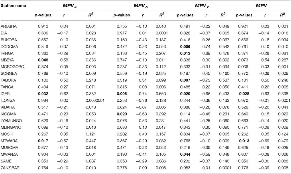
Table 1. Indicates p-values and Coefficients of determination (R²) for MPV, values in bold are statistically significance at alpha = 0.05.

TABLE 2

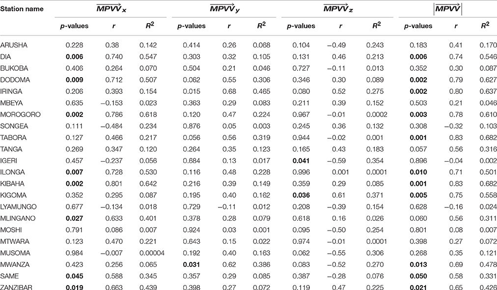
Table 2. Indicates p-values and Coefficients of determination (R²) for $\overrightarrow{MPVV}$ values in bold are statistically significance at alpha = 0.05.

The MPV_x has shown correlation coefficient of greater than or equal to 0.4 at 6 meteorological stations (Table 1), while ${\overrightarrow{MPVV}}_y$ has high correlation coefficient of greater or equal to 0.4 at 8 stations (Table 2). The MPV_y has correlated with rainfall with correlation coefficient of greater or equal to 0.4 at 7 stations (Table 1), while ${\overrightarrow{MPVV}}_z$ has correlation coefficient of greater or equal to 0.4 at 11 meteorological stations (Table 2). The MPV has relatively strong correlated with rainfall at 4 meteorological stations (Table 1). On the other hand $\left|\overrightarrow{MPVV}\right|$ has relatively strongly correlated with rainfall at 14 meteorological stations (Table 2). Overall, the findings implied that $\overrightarrow{MPVV}$ correlate better with rainfall than the MPV. Also ${\overrightarrow{MPVV}}_x$ and $\left|\overrightarrow{MPVV}\right|$ correlated better with rainfall than the other components.

The bivariate regression analysis to examine the predictive power between annual cycle rainfall as independent variable and the MPV and its terms are also presented in (Table 1). This table indicates that MPV_z explains better the variation of rainfall over Mbeya (R² = 0.336, p = 0.048), while MPV_x explain better the variation of rainfall over Igeri (R² = 0.550, p = 0.006). The MPV_y, explain better the variation of rainfall over Dodoma (R² = 0.542, p = 0.006), Iringa (R² = 0.478, p = 0.013), Tabora (R² = 0.537, p = 0.007), and Mwanza (R² = 0.348, p = 0.044). The MPV explain better the variation in rainfall only over Mtwara (R² = 0.479, p = 0.013).

On the other hand, the bivariate regression analysis is conducted to examine the predictive power between annual cycle rainfall as independent variable and the magnitude and the components of $\overrightarrow{MPVV}$ are presented in Table 2. Results showed that over Dar es Salaam (DIA), ${\overrightarrow{MPVV}}_x$ explains the variation of rainfall with (R²= 0.547, p = 0.006), followed by $\left|\overrightarrow{MPVV}\right|$ with (R² = 0.546, p = 0.006). ${\overrightarrow{MPVV}}_x$, explain better the variation of rainfall over Morogoro with (R² = 0.618, p = 0.002), Ilonga with (R² = 0.530, p = 0.007), and over Mlingano with (R² = 0.401, p = 0.027).

$\left|\overrightarrow{MPVV}\right|$ explain better the variation in rainfall over Dodoma (R² = 0.627, p = 0.002), Iringa (R² = 0.637, p = 0.002), Tabora (R² = 0.682, p = 0.001), Kibaha (R² = 0.682, p = 0.001), Kigoma (R² = 0.558, p = 0.005), Mwanza (R² = 0.478, p = 0.013) and Zanzibar (R² = 0.426, p = 0.021). Term3 better explain the variation of rainfall at Igeri (R² = 0.354, p = 0.041).

The variations of annual cycles in rainfall and ${\overrightarrow{MPVV}}_x$ over unimodal and bimodal regions represented by Tabora and Kibaha stations respectively are presented in Figures 2, 3. It is clear that ${\overrightarrow{MPVV}}_x$ catches the annual cycles of rainfall.

FIGURE 2

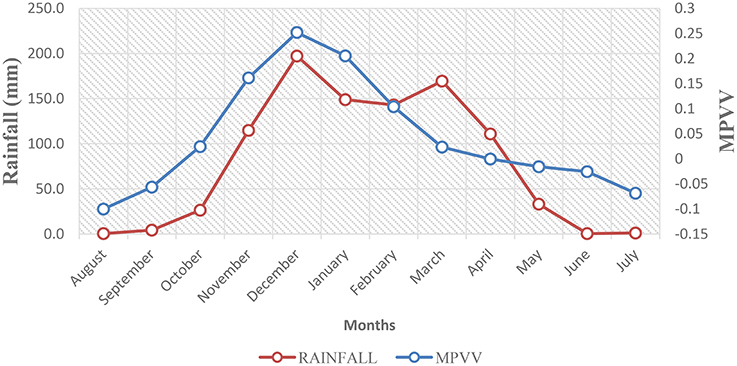
Figure 2. Annual cycle of rainfall and $\overrightarrow{MPV{V}_x}$ (10²*PV-units) at 700 hPa calculated from 1976-2001 at Tabora meteorological station.

FIGURE 3

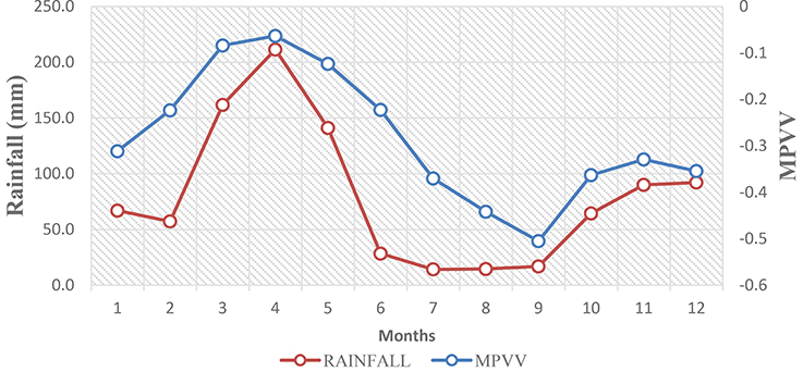
Figure 3. Annual cycle of rainfall and $\overrightarrow{MPV{V}_x}$ (10²*PV-units) at 700 hPa calculated from 1976-2001 at Kibaha meteorological station.

Summary and Recommendations

The aim of this study was to compute the moist potential vorticity (MPV) and moist potential vorticity vector $\overrightarrow{MPVV}$ and compare their performance in describing annual cycles of rainfall over different regions of Tanzania. Results indicated that $\overrightarrow{MPVV}$ perform better in explaining the variation of rainfall than MPV. ${\overrightarrow{MPVV}}_x$, and $\left|\overrightarrow{MPVV}\right|$ provide strong correlation coefficient with rainfall at significant level less than 0.05 at many stations when compared to other components. This suggests that ${\overrightarrow{MPVV}}_x$, and $\left|\overrightarrow{MPVV}\right|$ can be used as predictors of rainfall over different regions where they have shown strong correlation coefficient, and high coefficient of determination at significant level of 0.05. For instance, in Figures 2, 3 ${\overrightarrow{MPVV}}_x$ captured the annual cycle of rainfall over Tabora in unimodal region and Kibaha in bimodal region. One can construct a transfer function between ${\overrightarrow{MPVV}}_x$ and monthly rainfall and use it to improve climate projections for rainfall or for seasonal climate prediction. This is important especially for Tanzania where seasonal climate forecasting is based on analyzing analog years. This is the simple seasonal prediction technique based on analyzing weather maps that resemble other weather maps for different years within the season in the historical record and normally is based on subjective judgments from human eyes. This method produces fairly inaccuracy seasonal climate prediction (Huijun et al., 2015).

In this study we recommend the use of $\overrightarrow{MPVV}$ as predictor of annual cycles of rainfall over different regions in Tanzania. $\overrightarrow{MPVV}$, show the observed pattern of rainfall, that in MAM where there is higher rainfall total, $\overrightarrow{MPVV}$ is also higher and in OND where there is lower rainfall total, $\overrightarrow{MPVV}$ is lower too. Therefore a transfer function constructed based on $\overrightarrow{MPVV}$ may accurately predict the seasonal variation of rainfall over different regions in Tanzania.

Furthermore $\overrightarrow{MPVV}$ need to be explored more on its application to better seasonal prediction in East Africa where seasonal climate prediction depends among other techniques on simulations from the general circulation models (GCMs) forced by sea surface temperatures. However the GCMs have coarse space resolution to reproduce climate details at different regions. The results presented in this study contribute on the existing predictors that are used for development of empirical models for seasonal climate prediction. Most statistical model are constructed using predictors such as relative humidity, geo potential height, upper level wind speed (e.g., at 500 hPa). These predictors suffer to reproduce at the same time the dynamics and thermodynamics of the atmosphere. However $\overrightarrow{MPVV}$ reproduces at the same time the dynamics of atmospheric flows (through vorticity) and thermodynamics of atmospheric flows (through the gradient of moist entropy potential temperature).

It is important to note that the MPV and $\overrightarrow{MPVV}$ presented in this study were computed using data from the RCM driven by GCM. Therefore further studies are recommended to explore the performance of MPV and $\overrightarrow{MPVV}$ in describing rainfall events in Tanzania using data from RCM driven by ERA-Interim data. Moreover, it is recommended that $\overrightarrow{MPVV}$ should be tested on ability to reproduce interannual variability of rainfall to have more confidence to use it as predictor of rainfall events.

Author Contributions

The scientific contribution of both authors is significant to the manuscript, the computation and data search was done by PL. The validation of the model was done by GD. Both authors participated fully in writing and analyzing the results.

Conflict of Interest Statement

The authors declare that the research was conducted in the absence of any commercial or financial relationships that could be construed as a potential conflict of interest.

Acknowledgments

Authors are grateful to Tanzania Meteorological Agency, Rossby center for regional climate modeling, and the National Centers for Environmental Prediction/National Center for Atmospheric Research (NCEP/NCAR), for provision of data used in this study. Special thanks to Pascal Marquet from the Météo-France, CNRM/GMAP/PROC for the useful discussion on computation of his new novelty moist air entropic potential temperature.

References

Agrawala, S., Moehder, A., Hemp, A., Van Aalst, M., Hitz, S., Meena, H., et al. (2003). Development and Climate Change in Tanzania: Focus on Mount Kilimanjaro. Paris: OECD.

Google Scholar

Anyah, R. O., and Semazzi, F. H. M. (2007). Variability of East african rainfall based on multiyearRegCM3 simulations. Int. J. Climatol. 27, 357–371. doi: 10.1002/joc.1401

CrossRef Full Text | Google Scholar

Bechtold, P., Bazile, E., Guichard, F., Mascart, P., and Richard, E. (2001). A mass-flux convection scheme for regional and global models. Q. R. J. Meteorol. Soc. Vol. 127, 869–886. doi: 10.1002/qj.49712757309

CrossRef Full Text | Google Scholar

Benestad, R. E., Hanssen-Bauer, I., and Førland, E. J. (2007). An evaluation of statistical models for downscaling precipitation and their ability to capture long-term trends. Int. J. Climsyol. 27, 649–665. doi: 10.1002/joc.1421

CrossRef Full Text

Bennetts, D. A., and Hoskins, B. J. (1979). Conditional symmetric instability - a possible explanation for frontal rainbands. Q. J. R. Meteorol. Soc. 105, 945–962. doi: 10.1002/qj.49710544615

CrossRef Full Text | Google Scholar

Bjerknes, V. (1898a). Uber die Bildung von Circulationsbewegung und Wirbeln in reibungslosen Fliissigkeiten. Videnskabsselskapets Skrifter. I Math. Naturu. Klasse. 29.

Bjerknes, V. (1898b). Uber einen hydrodynamischen Fundamentalsatz und seine Anwendung besonders auf die Mechanik der Atmosphare und des Weltmeeres. Kgl. Suenska Vetenskapsakad. Handl. 31, 35.

Black, E. (2005). The relationship between indian ocean sea-surface temperature and east african rainfall. Philos. Trans. R. Soc. 1826, 43–47. doi: 10.1098/rsta.2004.1474

PubMed Abstract | CrossRef Full Text

Black, E., Slingo, J., and Sperber, K. R. (2003). An observational study of the relationship between excessively strong short rains in coastal east Africa and Indian ocean SST. Mon. Weather Rev. 131, 74–94. doi: 10.1175/1520-0493(2003)131<0074:AOSOTR>2.0.CO;2

CrossRef Full Text | Google Scholar

Cao, Z., and Cho, H.-R. (1995). Generation of moist potential vorticity in extratropical cyclones. J. Atmos. Sci. 52, 3263–3281.

Google Scholar

Charles, S. P., Bates, B. C., and Hughes, J. P. (1999). A spatio-temporal model for downscaling precipitation occurrence and amounts. J. Geophys. Res. 104, 31657–31669. doi: 10.1029/1999JD900119

CrossRef Full Text | Google Scholar

Chen, S. T., Yu, P. S., and Tang, Y. H. (2010). Statistical downscaling of daily precipitation using support vector machines and multivariate analysis J. Hydrol. 385, 13–22. doi: 10.1016/j.jhydrol.2010.01.021

CrossRef Full Text | Google Scholar

Daniels, A. E., Morrison, J. F., Joyce, L. A., Crookston, N. L., Chen, S. C., and McNulty, S. G. (2012). Climate projections FAQ. General Technical Report RMRS-GTR-277WWW. Fort Collins, CO: U.S. Department of Agriculture, Forest Service, Rocky Mountain Research Station, 32.

Danis, B., Laprise, R., Caya, D., and Cot^e, J. (2002). Downscaling ability of one-way nested regional climate models: the Big-Brother Experiment. Clim. Dyn. 18, 627–646 doi: 10.1007/s00382-001-0201-0

CrossRef Full Text | Google Scholar

Ertel, H. (1942). Ein Neuer hydrodynamischer Wirbelsatz. Met. Z. 59, 271–281.

Google Scholar

Fung, F., Lopez, A., and New, M. (2011). Modelling the Impact of Climate Change on Water Resources. Oxford: Wiley-Blackwell.

Google Scholar

Gao, S., Ping, F., Li, X., and Tao, W.-K. (2004b). A convective vorticity vector associated with tropical convection: a two-dimensional cloud-resolving modeling study. J. Geophys. Res. 109:D14106. doi: 10.1029/2004JD004807

CrossRef Full Text | Google Scholar

Gao, S., Wang, X., and Zhou, Y. (2004a). Generation of generalised moist potential vorticity in a frictionless and moist adiabatic flow. Geophys. Res. Lett. 31:L12113. doi: 10.1029/2003GL019152

CrossRef Full Text | Google Scholar

Goosse, H., Barriat, P. Y., Lefebvre, W., Loutre, M. F., and, Zunz, V. (2010). Introduction to Climate Dynamics and Climate Modeling. Available online at: http://www.climate.be/textbook

Hassan, Z., Shamsudin, S., and Harun, S. (2013). Application of SDSM and LARS-WG for simulating and downscaling of rainfall and temperature. Theor. Appl. Climatol. 116, 243–257. doi: 10.1007/s00704-013-0951-8

CrossRef Full Text | Google Scholar

Hewitson, B. C., and Crane, R., G (1996). Climate downscaling: techniques and application. Clim. Res. 7, 85–95.

Google Scholar

Hoskins, B. (1997). A potential vorticity view of synoptic development. Meteorol. Appl. 325–334.

Google Scholar

Hoskins, B. J., McIntyre, M. E., Robertson, A. W,and (1985). On the use and significance of isentropic potential vorticity maps. Q. J. R. Meteorol. Soc. 111, 877–946.

Google Scholar

Hoskins, B. J., and Sardeshmukh, P. D. (1987). A diagnostic study of the dynamics of the northern hemisphere winter of 1985/86. Q. J. R. Meteorol. Soc. 113, 759–778. doi: 10.1002/qj.49711347705

CrossRef Full Text | Google Scholar

Huijun, W., Ke, F., Jianqi, S., Shuanglin, L., Zhaohui, L., Guangqing, Z., et al. (2015). A review of seasonal climate prediction research in china. Adv. Atmos. Sci. 32, 149–168. doi: 10.1007/s00376-014-0016-7

CrossRef Full Text | Google Scholar

IPCC (2013). Summary for Policy, Makersand In: Climate, Change (2013). ”The Physical Science Basis,” in Contribution of Working Group I to the Fifth Assessment Report of the Intergovernmental Panel on Climate Change, eds T. F. Stocker, D. Qin, G. K. Plattner, M. Tignor, S. K. Allen, J. Boschung, et al. (New York, NY: Cambridge University Press).

Jones, R. G., Noguer, M., Hassell, D. C., Hudson, D., Wilson, S. S., Jenkins, G. J., et al. (2004). Generating High Resolution Climate Change Scenarios Using PRECIS. Exeter: Met Office Hadley Centre.

Liang, Z., Lu, C., and Tollerud, E. I. (2010). Diagnostic study of generalized moist potential vorticity in a non-uniformly saturated atmosphere with heavy precipitation. Q. J. R. Meteorol. Soc. 136, 1275–1288. doi: 10.1002/qj.636

CrossRef Full Text | Google Scholar

Luhunga, P., Botai, J., and Kahimba, F. (2016). Evaluation of the performance of CORDEX regional climate models in simulating present climate conditions of Tanzania. J. South Hemisphere Earth Syst. Sci. 66, 32–54. doi: 10.22499/3.6601.005

CrossRef Full Text | Google Scholar

Luhunga, P., Mutayoba, E., and Ng'ongolo, H (2014). Homogeneity of monthly mean air temperature of the United Republic of Tanzania with HOMER. Atmospher. Clim. Sci. 4, 70–77. doi: 10.4236/acs.2014.41010

CrossRef Full Text | Google Scholar

Marquet, P. (2011). Definition of a moist entropic potential temperature. Application to FIRE-I data flights. Q. J. R. Meteorol. Soc. 137, 768–791. doi: 10.1002/qj.787

CrossRef Full Text | Google Scholar

Marquet, P. (2014). On the de?nition of a moist-air potential vorticity. Q. J. R. Meteorol. Soc. 140, 917–929. doi: 10.1002/qj.2182

CrossRef Full Text | Google Scholar

Mayor, Y. G., and Mesquita, M. D. S. (2015). Numerical simulations of the 1 May 2012 deep convection event over cuba: sensitivity to cumulus and microphysical schemes in a high-resolution model. Adv. Meteorol. 2015:973151. doi: 10.1155/2015/973151

CrossRef Full Text | Google Scholar

McIntyre, M. E. (2015). “Potential Vorticity,” in Encyclopedia of Atmospheric Sciences, Vol 2, 2nd Edn., eds G. R. North (editor-in-chief), J. Pyle, and F. Zhang (New York, NY: Elsevier Science; Academic Press), 375–383.

McSweeney, C., New, M., and Lizcano, G. (2010). UNDP Climate Change Country Profiles: Tanzania. Available online at: http://www.geog.ox.ac.uk/research/climate/projects/undp-cp/UNDP_reports/Tanzania/Tanzania.lowres.report.pdf (Accessed May 10, 2013).

Mofor, L. A., and Lu, C. (2008). Generalized moist potential vorticity and its application in the analysis of atmospheric flows. Prog. Nat. Sci. 19, 285–289. doi: 10.1016/j.pnsc.2008.07.009

CrossRef Full Text | Google Scholar

Muchuru, S., Landman, W. A., DeWitt, D., and Lötter, D. (2014). Seasonal Rainfall Predictability over the Lake Kariba Catchment Area, Water SA Vol. 40. Available online at: http://www.wrc.org.za ISSN 0378-4738

Rangaswamy, R. (2006). Agricultural Statistics. New Delhi: New Age International (P) Ltd Publishers.

Google Scholar

Rossby, C. G. (1936). Dynamics of steady ocean currents in the light of experimental fluid mechanics. Pap. Phys. Oceanogr. 5, 1–43. doi: 10.1575/1912/1088

CrossRef Full Text | Google Scholar

Rossby, C. G. (1938). On the mutual adjustment of pressure and velocity distributions in certain simple current systems, II. J. Marine Res. 2, 239–263.

Rossby, C. G. (1939). Relation between variations in the intensity of the zonal circulation of the atmosphere and the displacements of the semi-permanent centers of action. J. Marine Res. 2, 38–55. doi: 10.1357/002224039806649023

CrossRef Full Text

Rossby, C. G. (1940). Planetary flow patterns in the atmosphere. Q. J. R. Meteorol. Soc. 66, 68–87.

Google Scholar

Roux, B. (2009). Ultra High-Resolution Climate Simulations over the Stellenbosch Wine Producing Region Using a Variable-Resolution Mode, MSc Dissertation, University of Pretoria. Available online at: http://upetd.up.ac.za/thesis/available/etd-11302009-185214/unrestricted/dissertation.pdf

Schubert, W., Ruprecht, E., Hertenstein, R., Nieto-Ferreira, R., Taft, R., Rozo?, C., et al. (2004). English translations of twenty-one of Ertel's papers on geophysical ?uid dynamics. Meteorolo. Zeitschrift. 13, 527–576. doi: 10.1127/0941-2948/2004/0013-0527

CrossRef Full Text | Google Scholar

Strandberg, G., Bärring, L., Hansson, U., Jansson,C., Jones, C., Kjellström, E., et al. (2014). CORDEX Scenarios for Europe from the Rossby Centre Regional Climate Model RCA4, Reports Meteorology and Climatology, 116SMHI, SE-60176 Norrköping, Sverige (2014)

Stoelinga, M. (1996). A potential vorticity-based study of the role of diabatic heating and friction in a numerically simulated cyclone. Mon. Wea. Rev. 124:849–874. doi: 10.1175/1520-0493

CrossRef Full Text | Google Scholar

Timiza, W. (2011). Climate Variability and Satellite – Observed Vegetation Responses in Tanzania. Master thesis Physical Geography and Ecosystem Analysis, Lund University, Seminar series 205, 30 ECTS.

Tumbo, S. D., Mpeta, E., Tadross, M., Kahimba, F. C., Mbillinyi, B. P., and Mahoo, H. F. (2012). Application of self-organizing maps technique in downscaling GCMs climate change projections for Same, Tanzania. J. Phys. Chem. Earth 35, 608–617. doi: 10.1016/j.pce.2010.07.023

CrossRef Full Text | Google Scholar

Vigaud, N., Vrac, M., and Caballero, Y. (2013). Probabilistic downscaling of GCM scenarios over southern India. Int. J. Climatol. 33, 1248–1263 doi: 10.1002/joc.3509

CrossRef Full Text | Google Scholar

Villegas, J. R., and Jarvis, A. (2010). Downscaling Global Circulation Model Outputs: The Delta Method Decision and Policy Analysis Working Paper No. 1, Centro internacional de agricultura Tropical

Wilby, L. R., and Fowler, J. H., (2011). Regional Climate Downscaling. Available online at: http://www.pages-perso-julie-carreau.univ-montp2.fr/UM2/Packages_and_Tutorial_files/downscaling.pdf

Wilby, R. L., and Wigley, T. M.L (2000). Precipitation predictors for downscaling: observed and general circulation model relationships. Int. J. Climatol. 20, 641–661. doi: 10.1002/(SICI)1097-0088(200005)20:6<641::AID-JOC501>3.0.CO;2-1

CrossRef Full Text | Google Scholar

Xiaoduo, P., Xin, L.i, Xiaokang, S. H. I., Xujun, H. A. N., Lihui, L. U. O., and Liangxu, W. A. N. G. (2012). Dynamic downscaling of near-surface air temperature at the basin scale using WRF–a case study in the Heihe River Basin,China. Front. Earth Sci. 6, 314–323. doi: 10.1007/s11707-012-0306-2

CrossRef Full Text

Yang, S., Gao, S. T., and Lu, C. G. (2014). A generalized frontogenesis function and its application. Adv. Atmos. Sci. 31, 1065–1078. doi: 10.1007/s00376-014-3228-y

CrossRef Full Text | Google Scholar

Zorita, E., and Von storch, H. (1999). The Analog method as a simple statistical downscaling technique: comparison with more complicated methods. J. Clim. 12, 2474–2489. doi: 10.1175/1520-0442(1999)012<2474:TAMAAS>2.0.CO;2

CrossRef Full Text | Google Scholar