New Advances in Dial-Lidar-Based Remote Sensing of the Volcanic CO2 Flux

Introduction

A major step forward in ground-based volcano monitoring has recently arisen from the advent of modern instrumental techniques and networks for volcanic gas observations (Galle et al., 2010; Oppenheimer et al., 2014; Saccorotti et al., 2014; Fischer and Chiodini, 2015). Such technical advances provide improved temporal resolution relative to traditional direct sampling techniques (Symonds et al., 1994; Giggenbach, 1996). As longer-term volcanic gas records increase in number and quality, full empirical evidence is finally emerging for increased CO₂ flux emissions prior to eruption of mafic to intermediate volcanoes (Aiuppa, 2015). Precursory plume CO₂ flux increases have been now detected at several volcanoes, including Etna (Aiuppa et al., 2008; Patanè et al., 2013), Kilauea (Poland et al., 2012), Redoubt (Werner et al., 2013), Turrialba (de Moor et al., 2016a), and Poas (de Moor et al., 2016b).

At Stromboli (in Italy), however, CO₂ flux observations have been particularly valuable for interpreting, and eventually predicting, the volcano's behavior (Aiuppa et al., 2010a, 2011). On Stromboli, the “regular” mild strombolian activity is occasionally interrupted by larger-scale vulcanian-style explosions, locally referred as “major explosions” or (in the most extreme events) “paroxysms” (Rosi et al., 2006, 2013; Andronico and Pistolesi, 2010; Pistolesi et al., 2011; Pioli et al., 2014). These explosions, although short-lived (tens of seconds to a few minutes), represent a real hazard for local populations, tourists and volcanologists, since they produce fallout of coarse pyroclastic materials over wide dispersal areas (Rosi et al., 2013). In addition, such events are not anticipated by any detectable anomaly in the geophysical or volcanological record, perhaps because they originate deep in the crustal roots of the volcano's' plumbing system (Bertagnini et al., 2003; Métrich et al., 2005, 2010; Allard, 2010). Observational evidence suggests, however, that “major explosions” (Aiuppa et al., 2011) and “paroxysms” (Aiuppa et al., 2010a) are both systematically preceded by days/weeks of anomalous CO₂-rich gas leakage from Stromboli's deep (8–10 km) magma storage zone (Aiuppa et al., 2010b). CO₂ flux emissions from the open-vent crater plume have become, therefore, a unique monitoring tool for volcanic hazard assessment and mitigation on the volcano.

On Stromboli, as at other volcanoes, the volcanic gas CO₂ flux is calculated from a combination of co-measured SO₂ fluxes and plume CO₂/SO₂ ratios (Burton et al., 2013; Aiuppa, 2015). While the SO₂ flux can remotely be sensed by UV spectroscopy (Oppenheimer, 2010; Oppenheimer et al., 2011), measuring the CO₂/SO₂ ratio requires in-situ direct sampling and/or measurements via Multi-GAS (Aiuppa et al., 2010a) or Fourier Transform Infra-Red Spectrometry (La Spina et al., 2013) in the vicinity of hazardous active vents. As such, implementation of novel techniques for the remote observation of the volcanic CO₂ flux, from more distal (and safer) locations, remains highly desirable.

New prospects for ground-based remote detection of the volcanic CO₂ flux have recently become available from the advent of a new lidar (Light Detection and Ranging) using the DIAL (Differential Absorption lidar) technique (Aiuppa et al., 2015; Fiorani et al., 2015, 2016). DIAL-lidars (Weitkamp, 2005; Fiorani, 2007) use backscattering of artificial light (laser) from atmospheric back-scatterers and/or from the volcanic plume itself, and are therefore potentially ideal for remote volcanic CO₂ detection (Fiorani et al., 2013; Queißer et al., 2015, 2016). In previous work, we demonstrated the ability of our lidar to remotely resolve the volcanic CO₂ flux from a relatively proximal measuring site (<200 m from the source vents) (Aiuppa et al., 2015). Here, we extend this work by reporting on a successful CO₂ flux detection at Stromboli over a far longer optical path (~3 km distance from the vents). Results of this proof-of-concept experiment confirm lidars as promising tools for remote monitoring of the volcanic CO₂ flux (Aiuppa et al., 2015; Queißer et al., 2016).

Materials and Methods

The Bridge Lidar

Our measurements on Stromboli (Figure 1) were obtained using the same DIAL-lidar described in Aiuppa et al. (2015) and Fiorani et al. (2015, 2016), and realized within the context of the FP7-ERC project Bridge (www.bridge.unipa.it). Only key information is reported here, and the reader is referred to previous studies for a detailed description of the instrument. In brief, the Bridge lidar (Figure 1D) uses a complex transmitter that integrates (i) an injection seeded Nd:YAG laser with (ii) a double grating dye laser. This transmitter is used to generate laser radiation at ~2010 nm, a region of the electromagnetic spectrum absorbed by atmospheric CO₂, while showing minimal cross-sensitivity to H₂O (Fiorani et al., 2013). At the ON and OFF wavelengths selected for this experiment, the differential cross section of CO₂ is five orders of magnitude larger than that of H₂O (Rothman et al., 2013). Considering a CO₂ mixing ratio of 400 ppm, and with the upper and lower ranges of H₂O mixing ratios used in atmospheric models (Berk et al., 2014), i.e., from 2.59% (tropics, sea level) to 0.141% (high latitude, winter, sea level), the respective CO₂ absorption is 3 and 5 orders of magnitude larger than that of H₂O. The 2.59% H₂O mixing ratio is not far from the saturated water vapor pressure at standard atmospheric conditions. We conclude that, even in a condensing volcanic plume, H₂O absorption is negligible compared to that of CO₂.

FIGURE 1

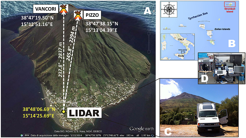
Figure 1. (A) Google Earth map of Stromboli volcano, showing positions of the measurement site (“LIDAR”) and of the Vancori and Pizzo peaks, see text; (B) Positioning of Stromboli relative to the mainland and the Aeolian archipelago; (C) the laboratory truck with the volcano summit in the background; (D) interior or the laboratory track.

A piezo-electric element is used to sequentially switch the wavelength of the transferred laser beam, from λ_ON (2009.537 mm: maximum CO₂ absorption) to λ_OFF (2008.484 nm: no CO₂ absorption), at 10 Hz repetition rate. These closely spaced pairs of laser beams are sequentially transmitted into the atmosphere, where they are eventually scattered back by atmospheric back-scatterers (aerosols, water droplets, particles) in either the volcanic plume or the background atmosphere. During their atmospheric propagation, the laser beams are also reflected by any obstacle encountered along the optical path, e.g., in our specific case, the Pizzo and Vancori walls/rims in front of or behind the volcanic plume (see Figures 1, 2). The returned signal is captured by the lidar receiver (a Newtonian telescope, diameter: 310 mm), and then detected and amplified by an InGaAs PIN photodiode module, directly connected with the analog-to-digital converter (ADC).

FIGURE 2

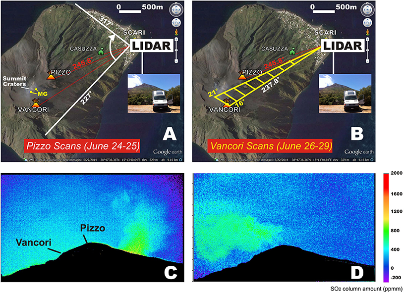
Figure 2. Maps illustrating geometries of (A) Pizzo scans and (B) Vancori scans. In the horizontal Pizzo scan in (A), the Field Of View (FOV) of the lidar was sequentially rotated (at constant elevation) at heading angles ranging from 227° to 317° (the Pizzo morphological peak was intercepted at ~245.8°). In (B), the heading angle was kept constant at 237.8°, while the plume was vertically profiled at elevations of 16 to 21°. (C,D) are pseudo-color images, from processing of UV camera data, showing distribution of SO₂ column amounts (in ppm m, see scale). The locations of Pizzo and Vancori are indicated in (C). During June 24–25, the UV camera images (see example in C) identified the plume as a nearly vertically rising band of peak SO₂ column amount, north of the Pizzo area; on June 26–29, the plume was instead transported south-southeast of Pizzo by the prevailing north-northwesterly winds (see image D).

Field Operations

During our experiment, the DIAL-lidar operated from a small laboratory truck (Figure 1C), positioned in a fixed position at the base of the volcano in the Scari area, ~2–2.5 km from the degassing vents on the volcano's summit (Figures 1, 2). The lidar operated during June 24–29, 2015, including an initial instrumental setup phase. Stable weather conditions (temperature, 22–26 °C; no rainfall) persisted during the entire measurement window.

During operations, two large motorized elliptical mirrors (major axis: 450 mm) simultaneously aimed the laser beams and the telescope, allowing the laser beam of the lidar to scan the volcanic plume either horizontally (Figure 2A) or vertically (Figure 2B). In particular, during June 24–25, the volcanic plume was mainly dispersed northwards by gentle southerly winds. From our Scari observation point (Figure 2), the plume was seen to rise nearly vertically north of the Pizzo area (Figure 2C). The Line Of Sight (LOS) of the lidar was therefore pointed north of Pizzo and the horizontal scan mode was preferred (heading angles: 227–317°; Figure 2A). Vertical scans above the Pizzo area were also performed. For simplicity, we refer below to these June 24–25 measurements as the Pizzo scans (Figure 2A).

On June 26–29, the plume was instead transported south-southeast by the prevailing north-northwesterly winds (Figure 2D). Vertical scans were therefore preferred that were operated at constant heading angle (237.8°) and at elevation angles from 16 to 21° (Figure 2B). In such conditions, the Pizzo and Vancori peaks were intercepted at elevation angles of 16.98° and 17.78°, respectively, and the volcanic plume was in all cases encountered in the 2300–2700 m range. We hereafter refer to these scans as the Vancori scans (Figure 2B).

During each profile, 100 lidar returns, 50 at λ_ON, 50 at λ_OFF, and interlaced (OFF after ON, OFF again and so on), were emitted at a 10 Hz rate, then co-added and averaged to increase the signal-to-noise ratio, reducing the signal sampling frequency to 0.1 Hz (temporal resolution of 10 s). The spatial resolution was about 5 m (corresponding to the rise time of the detector module due to its bandwidth). Plume scans, both horizontal and vertical, were retrieved combining about 50 profiles in <10 min. Typically, 10 scans at different elevations were repeated, obtaining a three-dimensional tomography of the volcanic plume.

A cell filled with standard CO₂ gas was periodically used during operations, for check of wavelength accuracy, repeatability and stability. In brief, our calibration procedure involved measuring-by photoacoustic spectroscopy—the absorption of the CO₂ gas cell as a function of wavelength. This calibration, limited to a small interval near the predicted λ_ON, allowed identifying the wavelength at which cell absorption is maximum. The laser system was finally forced to transmit at this radiation. The CO₂ absorption cross-section used in our calculations was based on HITRAN data (Rothman et al., 2013).

UV Camera

Concurrently with our lidar observations, a dual-UV camera system (Kantzas et al., 2010; Tamburello et al., 2012; Burton et al., 2014) was used to monitor the temporal variations of the SO₂ flux and plume transport speed. A fully autonomous system, similar to that used in other recent work (D'Aleo et al., 2016), was mounted on the roof of the laboratory truck and operated every day from 6 am to 4 pm (Local Time). The UV camera system acquired sequential images of the plume at ~0.5 Hz using two JAI CM 140 GR cameras. Both cameras had 10-bit digitization and 1392 × 1040 pixels, using an Uka Optics UV lens with a ~37° field of view. Distinct band-pass filters, centerd at either 310 nm (where SO₂ absorbs) or 330 nm (no SO₂ absorption), were mounted on the back on the lenses of the two cameras. Each set of co-acquired images from the two UV cameras was processed using the methodology of Kantzas et al. (2010) and integrated into the Vulcamera software (Tamburello et al., 2011, 2012), to calculate an absorbance for each camera pixel. Absorbance was converted into an SO₂ column amount from readings of a co-exposed Ocean optics USB2000+ UV Spectrometer, as outlined in Lübcke et al. (2013). Cameras and spectrometer were both controlled by a mini-pc Jetway. To calculate SO₂ flux time-series, we used Vulcamera to derive temporal records of SO₂ integrated column amounts (ICAs) along a plume cross-section, perpendicular to the plume transport direction. The obtained ICA time-series were then combined with high-temporal resolution (~1 Hz) records of plume transport speed. This latter was derived using an Optical Flow sub-routine using the Lukas/Kanade algorithm (Bruhn et al., 2005; Peters et al., 2015), integrated in Vulcamera. In our specific case, the Lucas-Kanade method was used to track movements of gas fronts (e.g., gas-rich and/or ash-free portions of the plume, having well distinct absorbance features) in consecutive UV camera frames, which allowed us quantifying plume transport speed at 0.5 Hz. We tested performance of this method by using artificial images with known particle velocities, and obtained errors in estimated velocities of <5%. Table 1 lists daily means (±1 SD: standard deviation) of both SO₂ fluxes and plume transport speed (V_p) during our observational period.

TABLE 1

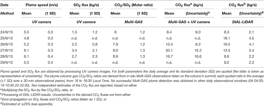
Table 1. Results of volcanic gas plume observations at Stromboli volcano, 24–29 June 2015.

Results

Characteristics of the DIAL-Lidar Signal

According to lidar theory (Fiorani, 2007), the optical power returned to the lidar receiver at any time t is produced by back-scattering of the laser beam by an atmospheric layer at distance R (range) from the source, where R = ct/2 and c is the speed of light. As such, the lidar offers range-resolved information on atmospheric structure and properties (aerosols, particles and gas molecules) along the laser beam, in the form of an intensity (I) vs. range plot (Figure 3).

FIGURE 3

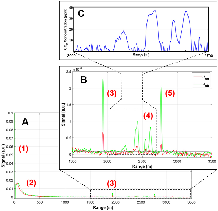
Figure 3. (A) Example of a lidar-based atmospheric profile, obtained at Stromboli during a typical Vancori scan, in the form of a range (distance) vs. signal intensity (arbitrary units, a.u.) plot. Peak (1) yields the pulse transmission zero-time (scattering, inside the laboratory truck, of some photons of the transmitted laser pulse); peak (2) is the returned signal from atmospheric back-scatterers along the laser optical path; peak (3) is the returned signal produced by reflection of the lidar beam by southeastern margin of the Pizzo morphological peak. (B) is a detail of (A), for ranges between 1500 and 3500 m. In this panel, peak (3) is as in (A); the series of peaks observed in the range interval 2300–2700 m (4) are due to back-scattering of the laser beam from the volcanic plume; peak (5) is produced by reflection of the laser beam by the Vancori peak; (C) a profile of in-plume excess CO₂ concentrations, in the 2000–2700 m range interval, calculated from processing of the lidar signal in (B). See text for the procedure used.

Upon its atmospheric propagation, the beam intensity decreases approximately (a) exponentially, due to atmospheric extinction, according to the Lambert-Beer law; and (b) as 1/R², because the solid angle subtended by the receiver is A/R², where A is the telescope's effective area. The two processes are superimposed. As such, in order to better observe the atmospheric back-scattering, a “range corrected signal, S” is commonly used, being given by: S = ln(I R²) (see below). Since the system works in DIAL mode, each intensity profile is in fact acquired at two distinct wavelengths, λ_ON–absorbed by CO₂–and λ_OFF–not absorbed by CO₂ (Figure 3). The two wavelengths are so close that atmospheric behavior, except from CO₂ absorption, is practically identical. The measured intensity contrast between the co-emitted λ_ON and λ_OFF signals allow range-resolved CO₂ concentrations in the volcanic plume to be obtained.

An example of a lidar-based atmospheric profile, obtained at Stromboli during a typical Vancori scan, is illustrated in Figure 3. As described above, the lidar registered one such profile every 10 s, since 100 lidar returns acquired at 10 Hz were co-added and averaged to increase the signal-to-noise ratio. Each of the atmospheric profiles (e.g., Figure 3) acquired during the Vancori scan contains the following characteristic features:

1) at R ~0, a first strong intensity peak is recorded for both λ_ON and λ_OFF (Figure 3A); this peak, which we refer to as I_{0, ON} and I_{0, OFF}, is due to scattering inside the laboratory truck of some photons of the transmitted laser pulse. This peak yields the pulse transmission zero-time, and its intensity is proportional to the transmitted energy (used for signal normalization),

2) for R between 0 and ~500 m, a weak signal is observed that is returned from atmospheric back-scatterers encountered by the laser beam along the optical path (Figure 3A); this signal, as explained before, attenuates with distance and vanishes at R ~500 m,

3) a I_{P, ON} and I_{P, OFF} peak at R ~1900 m (Figures 3A,B); this is produced by reflection of the lidar beam by the southeastern margin of the Pizzo morphological peak (see Figure 2),

4) a series of weak but resolvable peaks observed in the range interval 2300–2700 m (Figure 3B); in these peaks, the λ_ON signal appears strongly attenuated relative to the co-acquired λ_OFF signal, a fact due to laser absorption by CO₂ molecules in the volcanic plume,

5) a I_{V, ON} and I_{V, OFF} peak at R ~2800 m, which is produced by reflection of the laser beam by the Vancori peak (Figure 3B).

Atmospheric profiles obtained during the Pizzo scans of June 24–25 share similar characteristics, except that the Pizzo morphological peak is intercepted by the lidar beam at R ~2300 m, and the plume is encountered either before or after the Pizzo (Figure 4). The Vancori peak was obviously not encountered.

FIGURE 4

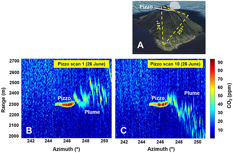
Figure 4. Example of two CO₂ concentration maps (B,C) obtained during a Pizzo horizontal scan on June 26. Geometry of the scans and location of the plume are schematically shown in (A). The maps show the distribution of CO₂ concentrations in the lidar's Field Of View (FOV), as a function of heading angle and range. Each map was obtained by interpolation of all CO₂ concentration profiles (e.g., same as 3A), obtained during a given Pizzo scan. In the maps, the red colored horizontal bands identify the margin of the Pizzo peak (heading angle: 244–245°), while the volcanic plume is the band of peak CO₂ concentration (up to 60 ppm) areas at heading angles of 245–250°.

Data Processing and Calculation of CO₂ Concentrations

We processed each acquired atmospheric profile using a Matlab analysis routine, with the aim of calculating the CO₂ concentrations in the atmospheric background and in the volcanic plume. The data processing routine consists of the following steps, all based on the Lambert-Beer law relation:

a) Initially, the CO₂ concentration in the natural background atmosphere, C₀, is calculated as:

$\begin{array}{cc}\ln \left[\frac{I_{P,OFF}/I_{0,OFF}}{I_{P,ON}/I_{0,ON}}\right]=2\Delta \sigma C_0{R}_P& \left(1\right)\end{array}$

where I_{P, ON} (I_{P, OFF}) stands for intensity of the ON (OFF) lidar signal [(3) in Figure 3A] caused by reflection of the laser beam off the surface of the Pizzo wall (R_P = 2294 m); I_{0, ON} (I_{0, OFF}) is the intensity of the ON (OFF) lidar peak caused by laboratory scattering of the laser pulse [(1) in Figure 3A]; and Δσ is the CO₂ differential absorption cross-section.

b) Secondly, ΔC, the average excess CO₂ concentration in the volcanic plume cross-section between Pizzo and Vancori [(3,5) in Figure 3B], is derived from:

$\begin{array}{cc}\ln \left[\frac{I_{V,OFF}/I_{P,OFF}}{I_{V,ON}/I_{P,ON}}\right]=2\Delta \sigma \left(C_0+\Delta C\right)\left(R_V-R_P\right)& \left(2\right)\end{array}$

Where I_{V, ON} (I_{V, OFF}) is the peak intensity of the ON (OFF) lidar signal caused by reflection of the laser beam off the surface of the Vancori rock wall (at R_V = 2837 m).

c) Thirdly, C_{CO2, i}, the excess CO₂ concentration corresponding to each i-th ADC channel of the lidar profile (Figure 3C) is calculated from:

$\begin{array}{cc}{C}_{CO2,i}=k{S}_i& \left(3\right)\end{array}$

$\begin{array}{cc}k=\frac{\Delta C\left(R_V-R_P\right)}{\Delta R{\displaystyle \sum _i{S}_i}}& \left(4\right)\end{array}$

$\begin{array}{cc}{S}_i=\ln \left(I_{i,OFF}{R}_i^2\right)& \left(5\right)\end{array}$

where ΔR is the range interval corresponding to each ADC channel, and I_{i, OFF} and R_i are the OFF lidar signal and the range of the i-th ADC channel (the OFF signal has been chosen because its signal-to-noise ratio is higher). Figure 3C shows an example of in-plume excess CO₂ concentration profile, obtained by applying the procedure above to the lidar profile of Figure 3B (in the 2100–2700 m range interval, where the volcanic plume was detected).

In-Plume CO₂ Concentration Maps

A series of CO₂ concentration profiles (one every 10 s), all similar to those shown in Figure 3C, were obtained as the volcanic plume was sequentially scanned by our DIAL-lidar, either horizontally or vertically, during the Pizzo/Vancori scans. By interpolating all CO₂ concentration profiles obtained during a single scan, we obtained sequences of CO₂ concentration maps, examples of which are shown in Figures 4, 5. Since a full scan of the plume was completed in ~1000–2000 s, each map is in fact obtained from the combination of ~50 to ~100 atmospheric profiles.

FIGURE 5

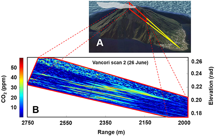
Figure 5. Example of a CO₂ concentration map (B) obtained during a Vancori vertical scan on June 26. Geometry of the scan and location of the plume is schematically shown in (A). The map shows the distribution of CO₂ concentrations in the lidar's FVO, as a function of range and elevation, and was obtained by interpolation of all CO₂ concentration profiles (e.g., same as 3A) obtained during a given Vancori scan. In the map, the volcanic plume corresponds to the cluster of high CO₂ concentrations (up to 60 ppmv) in the range interval 2200–2500 m and 0.2–0.22 rad (17–19.5°) elevations. The blue colored areas in the 2000–2000 m range correspond to near ambient (<10 ppm above background) CO₂ concentrations.

The maps illustrate the 2D distribution of CO₂ concentrations as a function of azimuth angle [°] (X axis) and range [m] (Y axis) for horizontal scans (Figure 4); or as a function of range [m] (X axis), and elevation angle [°] (Y axis) for the vertical scans (Figure 5). In both plots, the color scales (from blue to red) illustrate the level of CO₂ concentrations (in [ppm]) in the investigated space.

Figures 4, 5 demonstrate the ability of our DIAL-lidar to resolve in-plume volcanic CO₂ from the atmospheric background CO₂ (blue colors). In the CO₂ distribution maps, clusters of peak CO₂ concentration areas (marked by red, orange and yellow colors) identify the geometry of the plume. The lidar-based plume locations are consistent with visual and UV observations of volcanic plume dispersion (Figure 2). In the Pizzo horizontal scans, the plume was intercepted north of the Pizzo peak (heading angle: 244–245°), and is identified in the maps of Figure 4 as a cluster of peak CO₂ concentrations (up to 60 ppm above ambient air) at heading angles of 245–250°. The plume was detected over a relative wide range interval (R = 2000–2400 m), relative to the Pizzo peak (R ~2300 m). This is consistent with the slightly variable plume transport directions during our June 24–25 observation period that dispersed the plume either toward (Figure 4B) or away from (Figure 4A) the lidar observation point (R = 0). A few Pizzo vertical scans (not shown) confined the vertical extension of the plume to a diagonal band, extending from R = 2300 m and elevation ~19° (the Pizzo area) to R ~2700 m and ~20° elevation. Figure 5 is an example of a CO₂ distribution map obtained during a vertical Vancori scan. The map exhibits a clear volcanic plume signal, as marked by a cluster of high CO₂ concentrations (up to 60 ppm) in the range interval 2200–2500 m and 17–19.5° elevation. CO₂ remained at background air levels for range distances <2000 and >2800 m.

CO₂ Flux

The CO₂ concentration maps served as basis for calculating the CO₂ flux. To this aim, and by analogy with previous work (Aiuppa et al., 2015), we integrated the background-corrected (excess) CO₂ concentrations over the entire plume cross-sectional area covered by each scan, and multiplied this integrated column amount by the plume transport speed. Mathematically, the CO₂ flux (Φ_CO2, in kg·s⁻¹) was obtained from:

$\begin{array}{cc}{\Phi }_{{\text{CO}}_2}={\text{v}}_{\text{p}}·\frac{{\text{PM}}_{{\text{CO}}_2}}{{10}^3{\text{N}}_{\text{A}}}·{\text{N}}_{\text{molCO}2-\text{total}}& \left(6\right)\end{array}$

where v_P is the plume transport speed (in [m/s]) obtained from processing of UV camera images (Table 1); N_{molCO2−total} is the total-plume CO₂ molecular density (expressed in molecules m⁻¹); and PM_CO2 and N_A are, respectively, the CO₂ molecular weight and Avogadro's constant. The term N_{molCO2−total} was obtained by integrating the effective average excess CO₂ concentrations ($\overline{C_{exc,i}}$ [ppm]) over the entire plume cross section, according to:

$\begin{array}{cc}{N}_{molCO2-total}=N_h·{10}^{-6}·{\displaystyle \sum _i\overline{C_{exc,i}}·A_i}& \left(7\right)\end{array}$

where: N_h is the atmospheric number density (molecules m⁻³) at the crater's summit height, the term 10⁻⁶ converts $\overline{C_{exc,i}}$ into a dimensionless quantity, and A_i represents the i-th effective plume area, given by:

$\begin{array}{cc}{A}_i=l_i·\Delta R& \left(8\right)\end{array}$

where ΔR is the spatial resolution of the lidar (1.5 m) and l_i is the i-th arc of circumference (Figure 6B):

$\begin{array}{cc}{l}_i=R_i·\theta & \left(9\right)\end{array}$

FIGURE 6

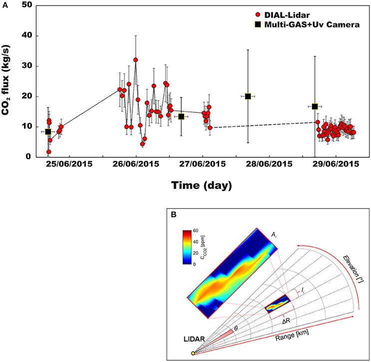
Figure 6. (A) Time-series of CO₂ fluxes from Stromboli volcano on June 24–29, 2015. Our DIAL-lidar based fluxes (red circles) were obtained using the procedure detailed in the text. For comparison, independent CO₂ flux estimates, obtained by multiplying the in-plume CO₂/SO₂ ratio (from Multi-GAS) by the SO₂ flux (from UV Cameras), are also presented. The two independent time-series are consistent (within error, see also Table 1). (B) Schematic plot defining the parameters used in the CO₂ flux calculation procedure (see text).

In relation (9), R_i is the i-th distance vector (in meters) and θ is the angular resolution of the system expressed in radians (ranging from 0.04° π/180 = 1.75 10⁻⁴ rad to 0.1° π/180 = 0.00175 rad) (Figure 6B).

Our obtained CO₂ fluxes, shown in Figure 6A, range from 1.8 to 32.1 kg/s. The lidar-based CO₂ flux time-series (Figure 6A) has maximum temporal resolution of 16–33 min (the time required to complete a full scan of the plume for our instrumental configuration). Temporal gaps in the dataset are caused by decreases in the signal-to-noise ratio (SNR) that prevent us from accurately detecting a clear CO₂ excess. These SNR decreases are likely caused by reduction of the backscattering coefficient of the probed air parcel, reflecting temporal variations in condensation extent of the volcanic gas plume. Visual (and UV camera) observations confirmed that the plume was variably condensed during our measurement interval, possibly due to slight changes in atmospheric conditions.

We evaluate the overall uncertainty in our derived CO₂ fluxes at ± 25% at 1s (see appendix).

Discussion

The scarcity of volcanic CO₂ flux data in the geological literature (see Burton et al., 2013 for a recent review) is a direct consequence of the technical challenges in resolving the volcanic CO₂ signal from the large atmospheric background (≈400 ppmv). In contrast to SO₂, which is present at the part per billion level in the background atmosphere, allowing the volcanic flux to be routinely measured from ground and space using UV spectroscopy (Oppenheimer, 2010), remote sensing of volcanic CO₂ has only been achieved during eruptions of mafic volcanoes. In such circumstances, magma/hot rocks can effectively be used as a light source for ground-based Fourier Transform Infra-Red (FTIR) spectrometers (Allard et al., 2005; Burton et al., 2007; Oppenheimer and Kyle, 2008). In contrast, measurement of the far more common “passive” CO₂ emissions from quiescent volcanoes has required access to hazardous volcano's summit craters for direct sampling of fumaroles (Fischer and Chiodini, 2015) or in-situ measurement of plumes via either Multi-GAS instruments (Aiuppa, 2015) or active-FTIR (Burton et al., 2000; La Spina et al., 2013; Conde et al., 2014).

A major breakthrough has recently arisen from the possible application of lidars to remote volcanic CO₂ sensing (Fiorani et al., 2013, 2015, 2016; Aiuppa et al., 2015; Queißer et al., 2015, 2016). Aiuppa et al. (2015) were the first to report on a DIAL-lidar-based remote measurement of the volcanic CO₂ flux at Campi Flegrei volcano, but their observations were limited to short (<200 m) measurement distances. Here, we have extended this earlier work to demonstrate that DIAL-lidars can successfully detect volcanic CO₂ at tens of ppmv above the atmospheric background over optical paths up to ≈3 km (Figures 4, 5). Similar results have recently been obtained at Campi Flegrei volcano by Queißer et al. (2016), suggesting that lidar may soon become an important operational tool in volcanic-gas research.

Our results constrain the CO₂ flux at Stromboli during June 24–29, 2015 (Figure 6A). Averaging all successful results during each measurement day, we obtain daily averages of the CO₂ flux between 8.3 ± 2.1 (June 24) and 18.1 ± 4.5 (June 25) kg/s, which correspond to cumulative daily outputs of 718 and 1565 tons, respectively. These results fall well in the range of previous CO₂ measurements on Stromboli. Aiuppa et al. (2010a, 2011) found that the CO₂ flux exhibits large temporal oscillations on Stromboli, from as low as 60 tons/day to as high as 11,000 tons/day, the highest values being observed in the days prior to paroxysmal and/or major explosions. The time-averaged CO₂ flux from Stromboli has been evaluated at 550 tons/day (Aiuppa et al., 2011) and at 1040–1200 tons/day (Allard, 2010). Our lidar-based CO₂ flux for the entire (June 24–29) measurement period is reasonably close, averaging at 1050 ± 250 tons/day (mean of 80 individual measurements).

Figure 6A offers further confirmation to the robustness of our results. In the figure, we compare our lidar-based CO₂ fluxes with independent estimates, in which the CO₂ flux was derived by multiplying the CO₂/SO₂ ratio of the plume by the SO₂ flux. This latter approach has been used at volcanoes for years (Aiuppa, 2015), and at Stromboli involves use of two fully automated Multi-GAS instruments, operating on the volcano's summit to measure the in-plume CO₂/SO₂ ratio (Figure 2A; Aiuppa et al., 2009, 2010a,b; Calvari et al., 2014). This is combined with SO₂ fluxes, delivered from either the FLAMES network of scanning UV spectrometers (Burton et al., 2009) or from UV camera observations (Tamburello et al., 2012), to obtain the CO₂ flux.

Problems with this Multi-GAS + SO₂ flux approach include issues of different temporal resolutions and poor temporal alignment of the two time-series. Successful Multi-GAS measurements of plume composition on Stromboli (Aiuppa et al., 2009, 2010b) are restricted to periods when the volcanic plume is dispersed by the local wind field into the Pizzo area, where the instruments are deployed (see Figure 2A). In addition, the Multi-GAS cannot operate continuously, but only during four equally spaced measurement cycles per day, each being 30 min long (Aiuppa et al., 2009). As such, the temporal resolution of the CO₂/SO₂ ratio time-series is 6 h at best. In contrast, the temporal resolution of UV spectrometers/cameras is higher, from ~10 to 20 min (Burton et al., 2009) to 0.5 s (Tamburello et al., 2012), but observations are intrinsically limited to daylight hours and to good meteorological conditions (no clouds).

Figure 7 exemplifies the issue related to misalignment between Multi-GAS and UV observations. In the June 26th example, the only successful Multi-GAS acquisition period (from 1600 to 1630 h local time) clearly did not overlap with the SO₂ flux acquisition window (0900 to 1600 h local time). To overcome this problem, the common practice is to average out available Multi-GAS and UV spectroscopy data to obtain daily means of the CO₂ flux (Aiuppa et al., 2010a). Owing to the large inter-daily variability of SO₂ flux (e.g., Figure 7), however, large uncertainties are associated with these derived CO₂ fluxes (see Table 1, and errors bars in Figure 6A).

FIGURE 7

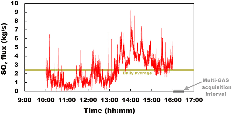
Figure 7. Temporal record of the volcanic SO₂ flux from Stromboli on June 26 th, 2015, as derived from our UV camera observations. The figure exemplifies misalignment between Multi-GAS and SO₂ flux time-series; plume CO₂/SO₂ ratios on June 26th were successfully measured only during the 1600–1630 local time Multi-GAS acquisition period, immediately after the end of the SO₂ flux acquisition window (0900–1600 local time). Poor temporal alignment is a flaw in the technique of estimating the CO₂ flux through a combination of Multi-GAS and UV camera records.

In spite of the issues above, we find overall consistency between the lidar-based and the traditional (Multi-GAS + UV spectroscopy-based) CO₂ fluxes (Figure 6A). This provides mutual validation for both quantification approaches. Our lidar-based CO₂ flux time-series (Figure 6A) are manifestly more continuous and of better temporal resolution (16–33 min). In addition, the lidar as with other remote sensing techniques is intrinsically safer. We caution, however, that further development is required before the lidar can become an operative tool for volcano monitoring. Improvements will need to occur in portability (the prototype weighs ~1100 kg), and reduced power requirement (6.5 kW) and costs (300 kUS $). In addition, the current measurement protocol is complex and thus requires great familiarity with the technique. Efforts are now being made to make the lidar more simple, user-friendly and fully automated, including development of an on-line remote control system and of a self-checking routine of the laser's wavelength settings. Electro-optics and laser/lidar private manufacturers need to be directly involved to transition the prototype into a more widely accessible, commercial instrument.

Conclusions

Our proof-of-concept study demonstrates the ability of DIAL-lidars to remotely (≈3 km distance) measure the volcanic CO₂ flux. Our reported lidar-based CO₂ fluxes at Stromboli volcano (1.8 ± 0.5 to 32.1 ± 8.0 kg/s) are in the same range as those obtained using standard techniques that require in-situ observations and are intrinsically more risky for operators. Our results, with those of Queißer et al. (2016), open new prospects for the use of lidars for instrumental remote monitoring of volcanic CO₂ flux. Further work is warranted in order to standardize and widen potential applications of Lasers in volcanic gas studies.

Author Contributions

AA, LF, and SS conceived the idea. AA, LF, SS, GM, and MN conducted the lidar/UV camera experiment. SP and RD processed the data, with help from AA, LF, and SS. ML provided the Multi-GAS results. AA drafted the manuscript with help from all co-authors.

Funding

The research leading to these results has received funding from the European Research Council under the European Union's Seventh Framework Program (FP7/2007/2013)/ERC grant agreement n 305377 (PI, Aiuppa), and from the DECADE-DCO research initiative.

Conflict of Interest Statement

The authors declare that the research was conducted in the absence of any commercial or financial relationships that could be construed as a potential conflict of interest.

Acknowledgments

Società Enel Produzione spa is kindly acknowledged for logistical support and for kindly providing access to “Centrale ENEL di Stromboli” during the field campaign. The authors wish to thank the Comune di Lipari, Circoscrizione di Stromboli, for authorizing use of the lidar on Stromboli.

References

Aiuppa, A. (2015). “Volcanic gas monitoring,” in Volcanism and Global Environmental Change, eds A. Schmidt, K. E. Fristad, and L. T. Elkins-Tanton (Cambridge: Cambridge University Press), 81–96.

Aiuppa, A., Bertagnini, A., Métrich, N., Moretti, R., Di Muro, A., Liuzzo, M., et al. (2010b). A model of degassing for Stromboli volcano, earth planet. Sci. Lett. 295, 195–204. doi: 10.1016/j.epsl.2010.03.040

CrossRef Full Text

Aiuppa, A., Burton, M., Allard, P., Caltabiano, T., Giudice, G., Gurrieri, S., et al. (2011). First observational evidence for the CO₂-driven origin of Stromboli's major explosions. Solid Earth 2, 135–142. doi: 10.5194/se-2-135-2011

CrossRef Full Text | Google Scholar

Aiuppa, A., Burton, M., Caltabiano, T., Giudice, G., Guerrieri, S., Liuzzo, M., et al. (2010a). Unusually large magmatic CO₂ gas emissions prior to a basaltic paroxysm. Geophys. Res. Lett. 37, L17303. doi: 10.1029/2010GL043837

CrossRef Full Text | Google Scholar

Aiuppa, A., Federico, C., Giudice, G., Giuffrida, G., Guida, R., Gurrieri, S., et al. (2009). The 2007 eruption of Stromboli volcano: insights from real-time measurement of the volcanic gas plume CO₂/SO₂ ratio. J. Volcanol. Geotherm. Res. 182, 221–230. doi: 10.1016/j.jvolgeores.2008.09.013

CrossRef Full Text | Google Scholar

Aiuppa, A., Fiorani, L., Santoro, S., Parracino, S., Nuvoli, M., Chiodini, G., et al. (2015). New ground-based lidar enables volcanic CO₂ flux measurements. Sci. Rep. 5:13614. doi: 10.1038/srep13614

PubMed Abstract | CrossRef Full Text | Google Scholar

Aiuppa, A., Giudice, G., Gurrieri, S., Liuzzo, M., Burton, M., Caltabiano, T., et al. (2008). Total volatile flux from Mount Etna. Geophys. Res. Lett. 35, L24302. doi: 10.1029/2008gl035871

CrossRef Full Text | Google Scholar

Allard, P. (2010). A CO₂-rich gas trigger of explosive paroxysms at Stromboli basaltic volcano, Italy. J. Volcanol. Geoth. Res. 189, 363–374. doi: 10.1016/j.jvolgeores.2009.11.018

CrossRef Full Text | Google Scholar

Allard, P., Burton, M. R., and Mure, F. (2005). Spectroscopic evidence for a lava fountain driven by previously accumulated magmatic gas. Nature 433, 407–410. doi: 10.1038/nature03246

PubMed Abstract | CrossRef Full Text | Google Scholar

Andronico, D., and Pistolesi, M. (2010). The November 2009 paroxysmal explosions at Stromboli. J. Volcanol. Geotherm. Res. 196, 120–125. doi: 10.1016/j.jvolgeores.2010.06.005

CrossRef Full Text | Google Scholar

Berk, A., Conforti, P., Kennett, R., Perkins, T., Hawes, F., and van den Bosch, J. (2014). “MODTRAN6: a major upgrade of the MODTRAN radiative transfer code,” in Proceedings SPIE 9088, Algorithms and Technologies for Multispectral, Hyperspectral, and Ultraspectral Imagery XX, 90880H (Baltimore, MD) (Accessed June 13, 2014).

Google Scholar

Bertagnini, A., Métrich, N., Landi, P., and Rosi, M. (2003). Stromboli an open window on the deep feeding system of a steady state volcano. J. Geophys. Res. 108, 2336. doi: 10.1029/2002JB002146

CrossRef Full Text | Google Scholar

Bruhn, A., Weickert, J., and Schnörr, C. (2005). Lucas/kanade meets horn/schunck: combining local and global optic flow methods international. J. Comput. Vis. 61, 211–231. doi: 10.1023/B:VISI.0000045324.43199.43

CrossRef Full Text | Google Scholar

Burton, M., Allard, P., Murè, F., and La Spina, A. (2007). Depth of slug-driven strombolian explosive activity. Science 317, 227–230. doi: 10.1126/science.1141900

PubMed Abstract | CrossRef Full Text | Google Scholar

Burton, M. R., Caltabiano, T., Murè, F., and Randazzo, D. (2009). SO₂ flux from Stromboli during the 2007 eruption: results from the FLAME network and traverse measurements. J. Volcanol. Geotherm. Res. 182, 214–220. doi: 10.1016/j.jvolgeores.2008.11.025

CrossRef Full Text | Google Scholar

Burton, M. R., Oppenheimer, C., Horrocks, L. A., and Francis, P. W. (2000). Remote sensing of CO₂ and H₂O emission rates from Masaya Volcano, Nicaragua. Geology 28, 915–918. doi: 10.1130/0091-7613(2000)28<915:RSOCAH>2.0.CO;2

CrossRef Full Text | Google Scholar

Burton, M. R., Prata, F., and Platt, U. (2014). Volcanological applications of SO₂ cameras. J. Volcanol. Geotherm. Res. 300, 2–6. doi: 10.1016/j.jvolgeores.2014.09.008

CrossRef Full Text | Google Scholar

Burton, M. R., Sawyer, G. M., and Granieri, D. (2013). Deep carbon emissions from volcanoes. Rev. Mineral. Geochem. 75, 323–354. doi: 10.2138/rmg.2013.75.11

CrossRef Full Text | Google Scholar

Calvari, S., Bonaccorso, A., Madonia, P., Neri, M., Liuzzo, M., Salerno, G. G., et al. (2014). Major eruptive style changes induced by structural modifications of a shallow conduit system: the 2007-2012 Stromboli case. Bull. Volcanol. 76, 1–15. doi: 10.1007/s00445-014-0841-7

CrossRef Full Text | Google Scholar

Conde, V., Robidoux, P., Avard, G., Galle, B., Aiuppa, A., Muñoz, A., et al. (2014). Measurements of SO₂ and CO₂ by combining DOAS, Multi-GAS and FTIR: study cases from Turrialba and Telica volcanoes. Int. J. Earth Sci. 103, 8, 2335–2347. doi: 10.1007/s00531-014-1040-7

CrossRef Full Text | Google Scholar

D'Aleo, R., Bitetto, M., Delle Donne, D., Tamburello, G., Battaglia, A., Coltelli, M., et al. (2016). Spatially resolved SO₂ flux emissions from Mt Etna. Geophys. Res. Lett. 43, 7511–7519. doi: 10.1002/2016GL069938

PubMed Abstract | CrossRef Full Text | Google Scholar

de Moor, J. M., Aiuppa, A., Avard, G., Wehrmann, H., Dunbar, N., Muller, C., et al. (2016a). Turmoil at Turrialba Volcano (Costa Rica): degassing and eruptive processes inferred from high-frequency gas monitoring. J. Geophys. Res. Solid Earth 121, 5761–5775. doi: 10.1002/2016JB013150

PubMed Abstract | CrossRef Full Text | Google Scholar

de Moor, J. M., Aiuppa, A., Pacheco, J., Avard, G., Kern, C., Liuzzo, M., et al. (2016b). Short-period volcanic gas precursors to phreatic eruptions: insights from Poás Volcano, Costa Rica. Earth Planet. Sci. Lett. 442, 218–227. doi: 10.1016/j.epsl.2016.02.056

CrossRef Full Text | Google Scholar

Fiorani, L. (2007). “Environmental monitoring by laser radar,” in Lasers and Electro-optics Research at the Cutting Edge, ed S. B. Larkin (Hauppauge, NY: Nova Science Publishers), 119–171.

Google Scholar

Fiorani, L., Santoro, S., Parracino, S., Nuvoli, M., Minopoli, C., Aiuppa, A., et al. (2015). Volcanic CO₂ detection with a DFM/OPA-based lidar. Opt. Lett. 40, 1034–1036. doi: 10.1364/OL.40.001034

PubMed Abstract | CrossRef Full Text | Google Scholar

Fiorani, L., and Durieux, E. (2001). Comparison among error calculations in differential absorption lidar measurements. Opt. Laser Technol. 3, 371–377. doi: 10.1016/S0030-3992(01)00041-X

CrossRef Full Text | Google Scholar

Fiorani, L., Saleh, W. R., Burton, M., Puiu, A., and Queißer, M. (2013). Spectroscopic considerations on DIAL measurement of carbon dioxide in volcanic emissions. J. Optoelectron. Adv. Mater. 15, 317–325.

Google Scholar

Fiorani, L., Santoro, S., Parracino, S., Maio, G., Nuvoli, M., and Aiuppa, A. (2016). Early detection of volcanic hazard by lidar measurement of carbon dioxide. Nat. Hazards 83, 21. doi: 10.1007/s11069-016-2209-0

CrossRef Full Text | Google Scholar

Fischer, T. P., and Chiodini, G. (2015). “Volcanic, magmatic and hydrothermal gas discharges,” in Encyclopaedia of Volcanoes, 2nd Edn, eds H. Sigurdsson, B. Houghton, S. McNutt, H. Rymer, and J. Stix (London: Academic Press; Elsevier), 779–797.

Google Scholar

Galle, B., Johansson, M., Rivera, C., Zhang, Y., Lehmann, T., Platt, U., et al. (2010). Network for Observation of Volcanic and Atmospheric Change (NOVAC)-A global network for volcanic gas monitoring: network layout and instrument description. J. Geophys. Res. 115:D05304. doi: 10.1029/2009JD011823

CrossRef Full Text | Google Scholar

Giggenbach, W. F. (1996). “Chemical composition of volcanic gases,” in Monitoring and Mitigation of Volcanic Hazards, ed R. Scarpa and R. J. Tilling (Heidelberg: Springer), 221–256.

Google Scholar

Kantzas, E. P., McGonigle, A. J. S., Tamburello, G., Aiuppa, A., and Bryant, R. G. (2010). Protocols for UV camera volcanic SO₂ measurements. J. Volcanol. Geotherm. Res. 94, 55–60. doi: 10.1016/j.jvolgeores.2010.05.003

CrossRef Full Text | Google Scholar

La Spina, A., Burton, M. R., Harig, R., Mure, F., Rusch, P., Jordan, M., et al. (2013). New insights into volcanic processes at Stromboli from Cerberus, a remote-controlled open-path FTIR scanner system. J. Volcanol. Geotherm. Res. 249, 66–76. doi: 10.1016/j.jvolgeores.2012.09.004

CrossRef Full Text | Google Scholar

Lübcke, P., Bobrowski, N., Illing, S., Kern, C., Alvarez Nieves, J. M., Vogel, L., et al. (2013). On the absolute calibration of SO₂ cameras. Atmos. Meas. Tech. 6, 677–696. doi: 10.5194/amt-6-677-2013

CrossRef Full Text | Google Scholar

Métrich, N., Bertagnini, A., and Di Muro, A. (2010). Conditions of magma storage, degassing and ascent at Stromboli: new insights into the volcano plumbing system with inferences on the eruptive dynamics. J. Petrol. 51, 603–626. doi: 10.1093/petrology/egp083

CrossRef Full Text | Google Scholar

Métrich, N., Bertagnini, A., Landi, P., Rosi, M., and Belhadj, O. (2005). Triggering mechanism at the origin of paroxysms at Stromboli (Aeolian archipelago, Italy): the 5 April 2003 eruption. Geophys. Res. Lett. 32:L103056. doi: 10.1029/2004GL022257

CrossRef Full Text | Google Scholar

Oppenheimer, C. (2010). Ultraviolet sensing of volcanic sulfur emissions, Elements 6, 87–92. doi: 10.2113/gselements.6.2.87

CrossRef Full Text | Google Scholar

Oppenheimer, C., Fischer, T. P., and Scaillet, B. (2014). “Volcanic Degassing: Process and Impact,” in Treatise on Geochemistry, The Crust, 4, eds H. D. Holland and K. K. Turekian (Amsterdam: Elsevier), 111–179.

Google Scholar

Oppenheimer, C., and Kyle, P. R. (2008). Probing the magma plumbing of Erebus volcano, Antarctica, by open-path FTIR spectroscopy of gas emissions. J. Volcanol. Geotherm. Res. 177, 743–754. doi: 10.1016/j.jvolgeores.2007.08.022

CrossRef Full Text | Google Scholar

Oppenheimer, C., Scaillet, B., and Martin, R. S. (2011). Sulfur degassing from volcanoes: source conditions, surveillance, plume chemistry and earth system impacts. in Sulfur in magmas and melts: its importance for natural and technical processes. Rev. Miner. 73, 363–422. doi: 10.2138/rmg.2011.73.13

CrossRef Full Text | Google Scholar

Patanè, D., Aiuppa, A., Aloisi, M., Behncke, B., Cannata, A., Coltelli, M., et al. (2013). Insights into magma and fluid transfer at Mount Etna by a multiparametric approach: a model of the events leading to the 2011 eruptive cycle. J. Geophys. Res. Solid Earth 118, 3519–3539. doi: 10.1002/jgrb.50248

CrossRef Full Text | Google Scholar

Peters, N., Hoffmann, A., Barnie, T., Herzog, M., and Oppenheimer, C. (2015). Use of motion estimation algorithms for improved flux measurements using SO2 cameras. J. Volcanol. Geotherm. Res. 300, 58–69. doi: 10.1016/j.jvolgeores.2014.08.031

CrossRef Full Text | Google Scholar

Pioli, L., Pistolesi, M., and Rosi, M. (2014). Transient explosions at open-vent volcanoes: the case of Stromboli (Italy). Geology 42, 863–866. doi: 10.1130/G35844.1

CrossRef Full Text | Google Scholar

Pistolesi, M., Donne, D. D., Pioli, L., Rosi, M., and Ripepe, M. (2011). The 15 March 2007 explosive crisis at Stromboli volcano, Italy: Assessing physical parameters through a multidisciplinary approach. J. Geophys. Res. Solid Earth 116, B12206. doi: 10.1029/2011JB008527

CrossRef Full Text | Google Scholar

Poland, M. P., Miklius, A., Sutton, J. A., and Thornber, C. R. (2012). A mantle-driven surge in magma supply to Kılauea Volcano during 2003-2007. Nat. Geosci. 5, 295–300. doi: 10.1038/ngeo1426

CrossRef Full Text | Google Scholar

Queißer, M., Burton, M., and Fiorani, L. (2015). Differential absorption lidar for volcanic CO₂ sensing tested in an unstable atmosphere. Opt. Express 23, 6634–6644. doi: 10.1364/OE.23.006634

CrossRef Full Text | Google Scholar

Queißer, M., Granieri, D., and Burton, M. (2016). A new frontier in CO₂ flux measurements using a highly portable DIAL laser system. Sci. Rep. 6:33834. doi: 10.1038/srep33834

CrossRef Full Text | Google Scholar

Rosi, M., Bertagnini, A., Harris, A. J. L., Pioli, L., Pistolesi, M., and Ripepe, M. (2006). A case history of paroxysmal explosion at Stromboli: timing and dynamics of the April 5, 2003 event. Earth Planet. Sci. Lett. 243, 594–606. doi: 10.1016/j.epsl.2006.01.035

CrossRef Full Text | Google Scholar

Rosi, M., Pistolesi, M., Bertagnini, A., Landi, P., Pompilio, M., and Di Roberto, A. (2013). Stromboli volcano, Aeolian Islands (Italy): present eruptive activity and hazards. Geol. Soc. Memoir 37, 473–490. doi: 10.1144/M37.14

CrossRef Full Text | Google Scholar

Rothman, L. S., Gordon, I. E., Babikov, Y., Barbe, A., Chris Benner, D., Bernath, P. F., et al. (2013). The HITRAN2012 molecular spectroscopic database. J. Quant. Spectrosc. Radiat. Transf. 130, 4–50. doi: 10.1016/j.jqsrt.2013.07.002

CrossRef Full Text | Google Scholar

Saccorotti, G., Iguchi, M., and Aiuppa, A. (2014). “In situ Volcano monitoring: present and future,” in Volcanic Hazards, Risks and Disasters, ed P. Papale (Amsterdam: Elsevier), 169–202.

Google Scholar

Symonds, R. B., Rose, W. I., Bluth, G. J. S., and Gerlach, T. M. (1994). Volcanic-gas studies: methods, results and applications. Rev. Mineral. Geochem. 30, 1–66.

Google Scholar

Tamburello, G., Aiuppa, A., Kantzas, E. P., McGonigle, A. J. S., and Ripepe, M. (2012). Passive vs. active degassing modes at an open-vent volcano (Stromboli, Italy). Earth Planet. Sci. Lett. 359, 106–116. doi: 10.1016/j.epsl.2012.09.050

CrossRef Full Text | Google Scholar

Tamburello, G., Kantzas, E. P., McGonigle, A. J. S., and Aiuppa, A. (2011). Vulcamera: a program for measuring volcanic SO₂ using UV cameras. Ann. Geophys. 54, 2. doi: 10.4401/ag-5181

CrossRef Full Text | Google Scholar

Weitkamp, C. (ed.). (2005). “Lidar: range-resolved optical remote sensing of the atmosphere,” in Springer Series in Optical Sciences, Vol. 102. (New York, NY: Springer).

Werner, C., Kelly, P. J., Doukas, M., Lopez, T., Pfeffer, M., McGimsey, R., et al. (2013). Degassing of CO₂, SO₂, and H₂S associated with the 2009 eruption of Redoubt Volcano, Alaska. J. Volcanol. Geotherm. Res. 259, 270–284. doi: 10.1016/j.jvolgeores.2012.04.012

CrossRef Full Text | Google Scholar

Appendix–Uncertainty and Error Analysis

Our lidar-based CO₂ fluxes are affected by the following error sources:

i. systematic error in CO₂ concentration measurement,

ii. statistical error in CO₂ concentration measurement,

iii. error in plume transport speed,

iv. error in identifying the integration area.

i. Systematic error of the CO₂ concentration measurement-It is well known that the DIAL-lidar systematic error is dominated by imprecision in wavelength setting (Fiorani et al., 2015), leading to inaccuracy in differential absorption cross section and thus in gas concentration. To minimize this error, we implemented a photo-acoustic cell filled with pure CO₂ at atmospheric pressure and temperature, close to the laser exit, in order to control the transmitted wavelength before each atmospheric measurement. This procedure allows us to set the ON/OFF wavelengths with better accuracy than the laser linewidth (Fiorani et al., 2016). Assuming that the error in the wavelength setting is ±0.02 cm⁻¹ (half laser linewidth), in the wavelength region used in this study, the systematic error of the CO₂ concentration measurement is 5.5%.

ii. Statistical error of the CO₂ concentration measurement - The statistical error has been calculated by standard error propagation techniques from the standard deviation of the lidar signal at each ADC channel. As discussed in Fiorani and Durieux (2001), the statistical error of the lidar signal increases with range. As a consequence, the uncertainty associated with the derived CO₂ concentrations also increases with range. In the distance range between Pizzo and Vancori, representing a mean measurement range, and at typical atmospheric and plume conditions encountered during this study, the statistical error of the CO₂ concentration measurement was about 2%. The statistical error exceed 5% at 4 km (well beyond our measurement range).

iii. Error in plume transport speed - The standard deviation and the average value of the wind speed have been calculated for each measurement session, and the corresponding relative error was evaluated (by error propagation technique) at 3%.

iv. Error in identifying the integration area - The integration area in which an excess CO₂ concentration is actually present is probably the most difficult parameter to retrieve accurately, and therefore represents the main error source in our calculated volcanic CO₂ fluxes. The following procedure has been followed. For each CO₂ concentration map (e.g., Figure 5), we initially measured: 1) A₁₅, the area where the excess CO₂ concentration was larger than 15 ppm; and 2) A₂₅ the area where the excess CO₂ concentration was larger than 25 ppm. Then, the average between A₁₅ and A₂₅ was taken as the best-estimated area, and their semi-difference as the error (~25%). The above thresholds have been chosen because below 15 ppm noise becomes significant, while above 25 ppm the plume area is reduced to its core. Use of a 15 ppm threshold likely underestimates the area (and thus the flux) of the order of magnitude of the measurement error, i.e., 10–20%.

Assuming that each error source is statistically independent, we can quadratically sum all the errors and obtain a cumulative error of ~ 25% (dominated by the area error).