Dynamic Changes at Yahtse Glacier, the Most Rapidly Advancing Tidewater Glacier in Alaska

1. Introduction

The rapid retreat and thinning of tidewater glaciers is governed by processes that can be substantially decoupled from climate (e.g., Post et al., 2011). The contributions to sea level rise from tidewater glaciers are highly variable and contribute to large uncertainties in sea level rise projections (Pachauri et al., 2014). Tidewater glaciers lose mass through a combination of surface ablation and frontal ablation (itself the sum of losses from submarine melt and iceberg calving). Mass loss is enhanced during tidewater glacier retreat due to dynamic thinning, in which accelerated flow leads to thinning of upstream ice followed by further acceleration (Meier and Post, 1987; Pfeffer, 2007). Dynamic thinning ends once a tidewater glacier terminus restabilizes, greatly reducing mass loss through frontal and surface ablation. While the prevalence and urgency of tidewater glacier retreat has resulted in comparatively well-studied retreat processes, the processes by which tidewater glaciers transition from retreat into a stable or advance phase are poorly understood (Post et al., 2011) despite their importance for developing long-term projections of sea level rise.

In the tidewater glacier advance and retreat cycle, advance is driven by a positive mass balance gained over a high accumulation-area ratio. For example, Hubbard Glacier, the largest nonpolar tidewater glacier in the world, is advancing at a rate of 35 m year⁻¹, has a mass balance of +0.32 Gt year⁻¹, and an accumulation-area ratio of 0.95 (Motyka and Truffer, 2007; Larsen et al., 2015; Mcnabb et al., 2015; Stearns et al., 2015). An important component of tidewater glacier advance is the presence, growth, and migration of a moraine shoal that protects the terminus from submarine melting and buoyancy driven instabilities (Powell, 1991). Repeat bathymetric studies at Hubbard glacier reveal the presence of a moraine shoal that advances at ~32 m year⁻¹, roughly the same rate as terminus advance (Goff et al., 2012). This supports the hypothesis that the rate of terminus advance is limited by the rate at which erosion and sedimentation can build and prograde the moraine shoal (Motyka et al., 2006). In a study modeling tidewater glacier advance, Nick et al. (2007) found that while positive mass balance and a high accumulation-area ratio can initiate the advance phase, the glacier could not advance into deep water without the presence of a moraine shoal. However, the development of the moraine shoal is generally considered to be a second-order process in tidewater glacier advance (Powell, 1991).

Yahtse Glacier, located in Icy Bay, southern Alaska (Figure 1), is currently advancing at ~100 m year⁻¹, making it the state's fastest-advancing tidewater glacier (Mcnabb and Hock, 2014). Yahtse formed in 1961 from a tributary that separated from the retreating Guyot Glacier and retreated until 1985, at which point Yahtse terminated at the foot of a steep (~35%) icefall (Porter, 1989). In 1990 Yahtse entered a phase of sustained advance at an average rate of ~100 m year⁻¹ (Mcnabb and Hock, 2014), which it maintains up to the time of writing. Repeat bathymetric soundings made 1.5 km from Yahtse's terminus show a 50 m shallowing between 1981 and 2011, evidence of sedimentation and the development of a moraine shoal (Post, 1983; Bartholomaus et al., 2013). However, Yahtse is unusual among advancing tidewater glaciers because it has been characterized by a negative mass balance and thinning in its accumulation zone–both before and after the initiation of its advance phase (Muskett et al., 2008; Larsen et al., 2015). Between 1972 and 2000, the portion of the upper basin located above 1220 m had an area-averaged thinning rate of −0.9 ± 0.1 m year⁻¹ (Muskett et al., 2008). The large upper basin continued to thin from 2006 to 2014, and despite thickening near the terminus yielded a −0.16 Gt year⁻¹ mass balance (Larsen et al., 2015). This large upper basin is connected to the narrow (~2.5 km wide) terminating fjord by the steep icefall. This icefall appears to have had a significant role in characterizing Yahtse's dynamic behavior. Following the separation from Guyot Glacier in 1961 (Porter, 1989), aerial photographs show that Yahtse's near-terminus region was much thicker and featured slopes that were more shallow than they are at present (Molnia, 2008), to such an extent that the icefall was mostly concealed. As Yahtse retreated, the constriction at the icefall likely limited the delivery of ice to the terminus, causing the terminus region to thin and steepen until it retreated to the base of the icefall. Similar stretching and thinning occurred near the terminus of Columbia Glacier as it approached a smaller icefall in 2001 although, unlike Yahtse, Columbia Glacier's retreat continued past its icefall (O'Neel et al., 2005). McNabb et al. (2012) suggested that the sharp change in ice thickness over a short horizontal distance at Columbia Glacier could keep regions on opposing sides dynamically decoupled by inhibiting the upstream transmission of stresses. In this paper, we investigate the major kinematic changes occurring at Yahtse on the decadal and seasonal scales to better understand the role of Yahtse's geometry in facilitating its rapid advance.

FIGURE 1

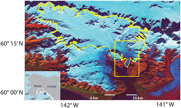
Figure 1. Regional map of Icy Bay and surrounding glaciers. Yahtse Glacier is outlined in yellow, and the study area containing Figures 2A, 6 is outlined by a yellow box. Map image is an October 17, 2014 Landsat 8 composite of bands 7, 5, and 3.

2. Data and Methods

2.1. Field Site

Our focus is on the lower section of Yahtse Glacier (Figure 1), specifically focusing on three points (A, B, and C) along the central flow line (Figure 2A). When referring to distances, we use a coordinate system in which the positive x-direction is along the central flow line and points in the upstream direction (Figure 2A). For analyses of velocity and ice elevations changes spanning multiple years, we use an Eulerian coordinate system in which the origin is at the intersection of the central flow line and the March 2014 terminus. Measurements are made at distances 1.25 and 3.5 km upstream from the terminus (positions A and B, respectively), and 2 km upstream from the top of the icefall (position C; Figure 2A). For analyses of interannual changes in driving stress and seasonal changes in velocity, we use a Lagrangian coordinate system with the origin placed at the intersection of the central flow line and the moving terminus. Distances 1.25 and 3.5 km upstream of the moving terminus position are labeled A′ and B′, respectively. By using a Lagrangian coordinate system, we avoid changes in the distance between reference points and the terminus (e.g., Howat et al., 2005).

FIGURE 2

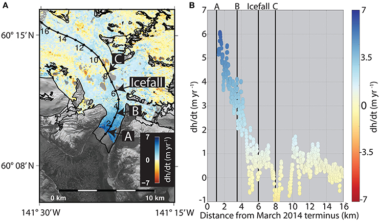
Figure 2. $\frac{\mathbf{d}\mathbf{h}}{\mathbf{d}\mathbf{t}}$ is shown for the region of Yahtse Glacier upstream of its February 2000 terminus position (A) and in profile along the center streamline (B). The locations of the icefall and Eulerian positions A, B, and C are marked by arrows, and the center streamline is shown by the black line with markers placed every 1 km (A).

2.2. Ice Elevation Change Rates

Ice elevation change rates ($\frac{dh}{dt}$) were estimated using a weighted linear regression with a horizontally and vertically coregistered “stack” of eleven Advanced Spaceborne Thermal Emission Reflection radiometer (ASTER) Digital Elevation Models (DEMs) that span the years 2000–2011, two WorldView DEMs that span the years 2012–2014, and the Shuttle Radar Topography Mission (SRTM) DEM collected during February 11-22, 2000. The acquisition dates and operational parameters of the images and satellites used are shown in Figure 3 and Table 1, respectively. The methods used are fully described by Melkonian et al. (2013, 2016) and Willis et al. (2012a), and are briefly described here.

FIGURE 3

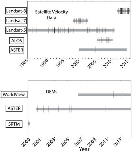
Figure 3. Acquisition dates of DEMs (top) used in elevation time series and satellite imagery used for estimating velocities (bottom). Gray horizontal bars indicate the operational period of each satellite. Black vertical lines show the acquisition dates of the DEMs.

TABLE 1

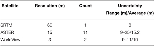
Table 1. Details of satellite imagery used in constructing the ice elevation time series.

The SRTM DEM was used as a base image because it is a C-band radar product and is therefore not affected by cloud and snow coverage that can yield spurious elevations in the optical ASTER and WorldView DEMs. WorldView and ASTER DEMs were down-sampled to 60 m resolution and horizontally and vertically coregistered to off-ice elevations from the SRTM DEM using the Ames Stereo Pipeline toolkit (Broxton and Edwards, 2008; Shean et al., 2016). Off-ice pixels were identified using the glacier and rock outlines provided by the Randolph Glacier Inventory (version 4.0; Pfeffer et al., 2014). We assigned 1σ uncertainty to each DEM using the difference between the ASTER or WorldView DEM and the SRTM DEM off-ice elevations. Uncertainties of the ASTER DEMs range from 9 to 25 m and are 15.2 m on average, while Worldview DEMs uncertainties range from 9-11 m and have an average of 10 m (Table 1). We assigned an initial 5 m uncertainty to the SRTM DEM following Carabajal and Harding (2005) and Rodriguez et al. (2006). Because the SRTM DEM is a C-band radar product, it is subject to snow and ice penetration that must be corrected before it is included in the DEM time series (e.g., Willis et al., 2012b; Melkonian et al., 2014; Berthier et al., 2016). Previous studies in the Juneau Icefield and Southern Patagonian Icefield found that the C-band SRTM DEM has a maximum penetration depth of 2-3 m in these regions compared to its X-band counterpart which, due to its smaller wavelength, is assumed to have a relatively small radar penetration depth (Willis et al., 2012b; Melkonian et al., 2014). Icy Bay, the Juneau Icefield, and the Southern Patagonian Icefield are similar in that they are regions of temperate glaciers with high mass-turnover rates. We therefore used 3 m as a conservative estimate of the uncertainty in the SRTM DEM's penetration depth, yielding a total uncertainty of 8 m (Table 1). Further work is needed to determine if this method under-estimates the penetration depth of the radar in Alaska, a situation that has been suggested to occur in the European Alps (Berthier et al., 2016).

We calculated $\frac{dh}{dt}$ values on a pixel-by-pixel basis by running a linear regression in which each elevation value is weighted by the inverse of the DEM uncertainty. We expect that the greatest elevation changes occur in the region of the advancing/retreating termini of Yahtse and Guyot Glaciers and used an iterative approach to identify an upper bound of +10 m year⁻¹ and lower bound of -30 m year⁻¹ for the $\frac{dh}{dt}$ in these regions. We filtered spurious elevations resulting from cloud coverage by excluding elevations from the final regression that deviate by more than ${}_{-30}^{+10}$ m year⁻¹ from the first elevation in the time series. Because Yahtse is advancing into the ocean, regions between the most advanced and retracted terminus positions in the DEM time series will show a positive $\frac{dh}{dt}$ that does not necessarily represent ice thickening. We therefore limited $\frac{dh}{dt}$ results to regions upstream of the terminus as mapped in 2000 by the SRTM. We do not apply any correction for seasonal changes in elevation, as each DEM has an uncertainty ranging from 8 to 25 m (Table 1), and it is unclear that any seasonal change could be resolved (e.g., Wang and Kääb, 2015). Although the noise on individual ASTER DEMs is large, the time series approach using multiple dates spread over different seasons overcomes some of the issues of differencing only two DEMs, without applying seasonal corrections (Willis et al., 2012a; Wang and Kääb, 2015; Berthier et al., 2016). Finally, we limited $\frac{dh}{dt}$ results to pixels with a stack of at least seven DEMs to improve accuracy.

2.3. Bathymetry

Bathymetric soundings from 1981, shortly before the glacier reached its most retracted position (Post, 1983) were manually georeferenced and contoured using GDAL (http://www.gdal.org) and interpolated using Generic Mapping Tools (GMT; Wessel et al., 2013). However, the elevations of more recent glacier beds likely have changed since 1981 due to rapid erosion and sedimentation. Soundings made 1.5 km from the terminus in 2011 show a shallowing of 50 m compared to the 1981 soundings (Bartholomaus et al., 2013). We therefore assigned the glacier bed a crude time-dependent uncertainty estimate by assuming that the bathymetry has changed at a linear rate since the terminus began advancing in 1990. The uncertainty σ in meters as function of the year of interest t is

$\begin{array}{ll}\sigma =50\frac{t-1990}{2011-1990}& (1)\end{array}$

This uncertainty reflects the ability of the advancing terminus to override or entrench itself in proglacial sediments (e.g., Kuriger et al., 2006; Motyka et al., 2006). Because deposition and erosion can both modify the elevation of the glacier bed, we do not make any assumptions as to whether the glacier bed has shallowed or deepened over time. We then used overridden seafloor topography for estimating the ice thickness and driving stress.

2.4. Driving Stress

Driving stress was calculated along the center streamline using a March 23, 2014 WorldView DEM, April 1, 2006 ASTER DEM, and the February 11-22, 2000 SRTM DEM with the gridded bathymetry. Topography was smoothed with a 400 m moving average, and surface slope was smoothed with a 1 km moving average to account for longitudinal coupling of resistive stresses (e.g., O'Neel et al., 2005). Ice thickness H was found as the difference between the ice surface topography and overridden bathymetry, and driving stress τ_D was calculated as

$\begin{array}{ll}{\tau }_D={\rho }_{i}gH\text{ sin}(\alpha )& (2)\end{array}$

where ρ_i is the density of ice (917 kg m⁻³), g is acceleration due to gravity (9.8 m s⁻²), and α is the surface slope (e.g., Cuffey and Paterson, 2010).

2.5. Ice Velocities

We estimated horizontal ice velocities from 1985 to 2016 using pixel-tracking techniques with 163 ALOS, ASTER, and Landsat 5, 7, and 8 satellite image pairs. The acquisition dates of the imagery and the operational parameters for each satellite are summarized in Figure 3 and Table 2. ASTER images were orthorectified to their own DEM by Land Processes Distributed Active Archive Center (LPDAAC). Landsat 5, 7, and 8 imagery were provided orthorectified by the United States Geologic Survey (USGS). Raw ALOS SAR imagery were prepared for pixel-tracking using the Repeat Observation Interferometry PACkage (ROI_PAC: Rosen et al., 2004).

TABLE 2

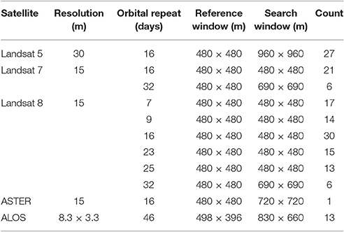
Table 2. Operational parameters for satellite images used in velocity time series.

Once the images were orthorectified and prepared, we performed pixel-tracking through normalized cross-correlation using the “ampcor” function of the ROI_PAC software as implemented by Melkonian et al. (2014). Uncertainties for each velocity pair were calculated as the median velocity of the off-ice portions, which should be zero (e.g., Willis et al., 2012a), and velocity maps with uncertainties >0.5 m day⁻¹ were excluded from the time series. The average uncertainty of the velocities used in the time series is 0.25 m day⁻¹. Full details on the methods used for filtering and other post processing are described by Willis et al. (2012a); Melkonian et al. (2013, 2016). We sampled velocities along a center streamline by taking the median within a 500 m section of the center streamline centered positions A, B, and C (Figure 2A).

Strain rates were calculated in the UTM coordinate system and then projected into the flow line coordinate system, in which the x-axis is aligned with ice flow and the y-axis is in the cross-flow direction. We use a sign convention in which longitudinal compression is negative. Due to the lower image quality of optical imagery predating the launch of the Landsat 8 satellite (e.g., Jeong and Howat, 2015) and the narrow shape of the terminus, we were only able to obtain useful strain rates in the region surrounding the center flow line. We assume that a 1D measurement of strain rates is a good approximation, as we are primarily interested in longitudinal strain rates, and the narrow shape of the terminus limits cross-flow variations.

2.6. Terminus Position

We tracked the terminus position at the centerline using the “Box Method” (e.g., Moon and Joughin, 2008; Mcnabb and Hock, 2014) with the Landsat images. In this method, we constructed a three-sided box formed by a fixed gate and sides that extend to a digitized terminus outline. The average length between the gate and the terminus was found by dividing the area of the box by the gate's width. Terminus shape was measured by outlining the terminus in the imagery manually. Because we are only interested in the qualitative changes in the terminus shape, we fit a smooth line to the terminus outline. Only cloud-free images are used in this study, and of those, only a sample are used to illustrate the seasonal changes in terminus shape.

3. Results

3.1. Interannual Changes

3.1.1. Geometry and Driving Stress

Two patterns of $\frac{dh}{dt}$ occur on alternate sides of the icefall (Figure 2). Upstream of the icefall, $\frac{dh}{dt}$ is small and uniform along the centerline (±1.5 m year⁻¹). Downstream of the icefall, $\frac{dh}{dt}$ increases at a linear rate and is greatest closest to the terminus (Figure 2B). Ice thickness did not change significantly between the years 2000 (277 ± 32 m) and 2014 (294 ± 66 m), however surface slopes near the terminus decreased by ~70% (Figure 4) and are correlated with a high positive $\frac{dh}{dt}$. Using Equation 2, we found that this decrease in slope drove a 60 ± 20% decrease in the driving stress along the first 500 m of the terminus between 2000 and 2014 (Figure 5). The terminus widened by ~8% between 2000 and 2014, however due to uncertainties in the topography and bathymetry we did not find a significant change in the cross-sectional area and therefore did not observe a significant amount of lateral spreading that could contribute to the observed kinematic changes on the decadal scale.

FIGURE 4

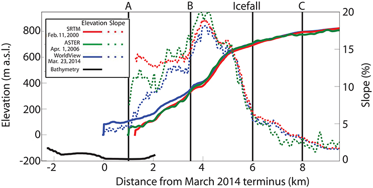
Figure 4. Elevation and slope sampled along the center streamline for the February 11–22, 2000, SRTM, April 1, 2006 ASTER, and March 23, 2014 WorldView DEMs. Bathymetry (Post, 1983) is shown in black. Vertical black lines show the locations of the icefall and Eulerian positions A, B, and C.

FIGURE 5

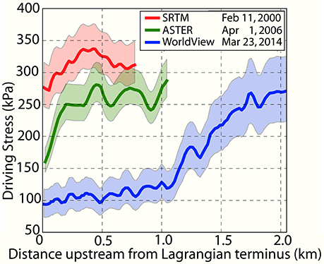
Figure 5. Driving stress at the terminus in a Lagrangian coordinate system for February 11–22, 2000, April 1, 2006, and March 23, 2014 with uncertainty shown in the shaded regions. Driving stress along the first 750m upstream from the terminus decreased by 60 ± 20% between 2000 and 2014. Driving stress is calculated for a greater distance upstream of the terminus in 2014 than in previous years because in 2014 the terminus had overlapped a greater portion of the bathymetry.

3.1.2. Velocities

As ice flows across the icefall, it is accelerated from 2–5 m day⁻¹ to 15–20 m day⁻¹ (Figure 6), in agreement with the results of Burgess et al. (2013a) and Bartholomaus et al. (2013). Separating velocity results by season shows that while position B decelerated by ~40% between 1996 and 2016 at a linear rate of −0.39 m day⁻¹ year⁻¹, there was no significant decadal trend in velocities at position C during this time (Figure 7B; Tables 3, 4). Spring-time (March – May) velocity profiles from 2000 to 2016 (Figure 7A) show that the rate of deceleration was higher for regions closer to the terminus than at position B. Between 2000 and 2016, longitudinal strain rates averaged between 2.5 and 3.5 km in the Eulerian coordinate system transitioned from a tensile strain rate regime to one of compression (Figure 8).

FIGURE 6

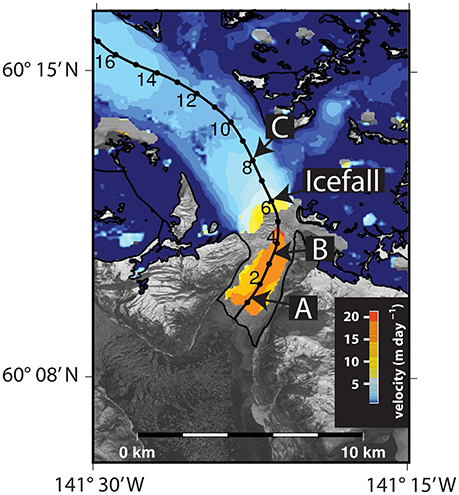
Figure 6. Ice velocity derived from pixel tracking with Landsat 8 images spanning March 7–23, 2014 chosen as a representative sample of the data set. The locations of the icefall and Eulerian positions A, B, and C are marked by arrows. Velocities are overlain on a panchromatic March 23, 2014 Landsat 8 image.

FIGURE 7

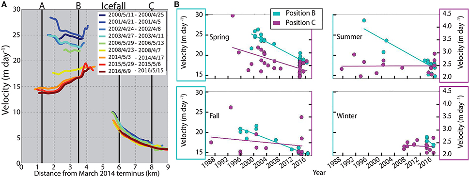
Figure 7. Velocity profiles for select spring months (March-May) for years with velocity coverage downstream of the icefall (A), and timelines of velocities separated by season and sampled at Eulerian positions B and C (B). Left and right vertical axes of (B) are at different scales, in which right axes (magenta) correspond to velocities sampled at C and left axes (cyan) correspond to velocities sampled at B. Statistics of the regression are shown in Tables 3, 4.

TABLE 3

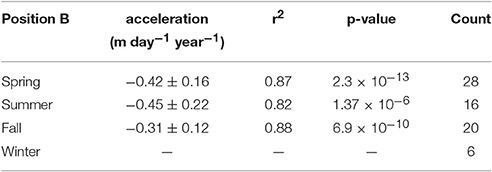
Table 3. Statistics for linear regression of velocities measured at position B.

TABLE 4

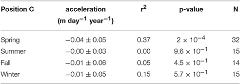
Table 4. Statistics for linear regression of velocities measured at position C.

FIGURE 8

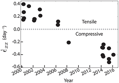
Figure 8. Longitudinal strain rates averaged from 2.5 to 3.5 km along the centerline in the Eulerian coordinate system. Positive values are tensile and negative values are compressive.

3.2. Seasonal Variations

3.2.1. Velocities

Velocity profiles for November 2013 – November 2014 are shown in Figure 9A, and the timelines of velocities at positions A′, B′, and C for years 2013–2016 are shown in Figure 9B. Seasonal velocity variations at position C increased during the spring, peaked in early June, and decelerated to a minimum in September (Figure 9B). Downstream of the icefall, a different pattern emerges. At A′ the timing of maximum velocity in 2013–2014 occurred when the terminus was in a retracted position in the winter (Figures 9B, 10B). Deceleration at A′ between February and June was synchronous with a ~200 m advance of the terminus. Further upstream at B′, velocities remained high during the winter and spring before they reached a maximum in early June and decreased throughout the summer (Figure 9B). The minima of all positions occurred in the fall. The 2013–2014 seasonal velocity pattern downstream of the icefall appears to be anticorrelated with the seasonal advance and retreat of the terminus and superimposed on the pattern observed at C. This effect is highest at A′, where the maximum speed occurred during the winter and decayed with distance upstream, resulting in the sustained high speeds during the winter and spring at B′. We cannot test whether or not the 2013–2014 A′ pattern is a regularly occurring event due to the limited number of winter and spring velocities in 2015 and 2016 (Figure 9B).

FIGURE 9

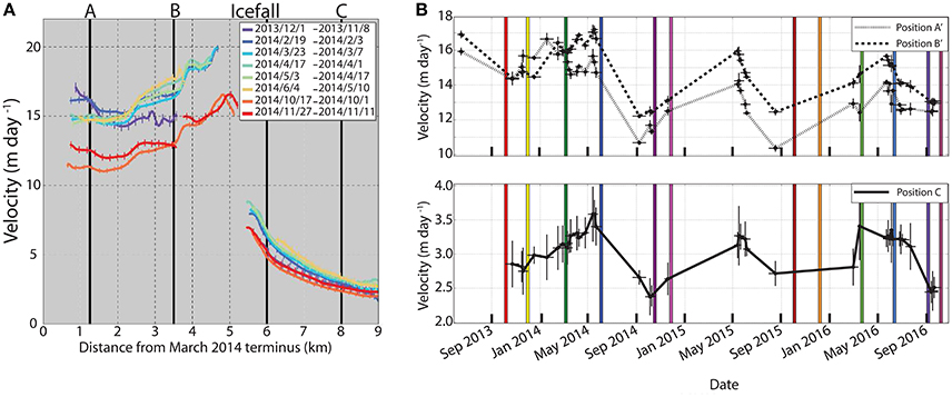
Figure 9. Centerline velocity profiles from Nov. 2013 to Nov. 2014 (A), and timeline of velocities sampled at three positions: Lagrangian A′ and B′ and Eulerian position C (B). Horizontal black bars show the time span of the image pairs, and vertical ticks show velocity uncertainty. Vertical black lines in (A) show the location of the icefall and Eulerian positions A, B, and C, and vertical colored lines in (B) correspond to the terminus outlines in Figure 10A.

FIGURE 10

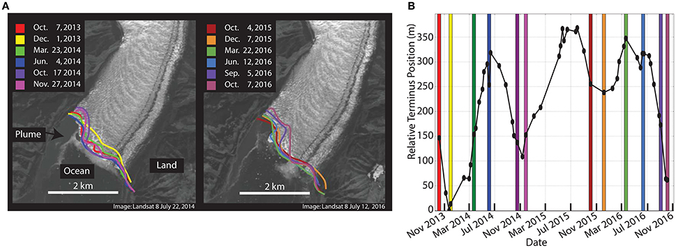
Figure 10. Select terminus configurations from Oct. 2013 - Nov. 2014 to Oct. 2015 - Oct. 2016 outlined from Landsat 8 imagery (A), and seasonal advance and retreat averaged across the terminus using the ‘Box Method’ (B). Vertical colored lines in (B) correspond to terminus outlines in (A).

3.2.2. Terminus Position and Shape

Figure 10B shows the seasonal terminus position calculated using the ‘Box Method’ and represents the seasonal advance and retreat averaged over the entire width of the terminus. On average, the terminus retreated from the early-summer to late-fall and advanced from mid-winter to the early-summer. The shape of the terminus changed from smooth in the winter and spring to crenulated in June due to the development of a calving embayment on the western edge in 2014 and 2016 (Figure 10A). The embayment in each year grew during the summer and reached a maximum size in October (Figure 10A). A similar calving embayment and locus of turbid discharge appeared and developed during the melt season of 2000 and 2015 (not shown), and was observed previously by Bartholomaus et al. (2013) at Yahtse in September 2011 (see Figure 1B of the referenced paper). As the embayment grew throughout the summer, the remaining portions of the terminus remained at their advanced position. A comparison between the timeline of average terminus positions (Figure 10B) and the terminus outlines (Figure 10A) shows that, although the width-averaged terminus position retreated during the summer, this was due to the growth of the calving embayment. The terminus did not retreat across its entire width until October – November (Figure 10A).

4. Discussion

4.1. Seasonal Dynamics

Although C is positioned ~8 km upstream of the March 2014 terminus and 2 km upstream of the icefall, the seasonality of velocities at C is similar to that reported near the termini of other Alaskan tidewater glaciers (e.g., Mcnabb et al., 2015; Stearns et al., 2015) — velocities are highest in late spring/early summer, at a minimum in the late fall, and intermediate during the winter. Spring acceleration is thought to be caused by surface meltwater that reaches an inefficient subglacial hydrologic system, leading to increased basal water pressure, increased separation at the ice-bed interface, and accelerated glacier sliding speeds (Iken and Bindschadler, 1986; Schoof, 2010). Over the course of the melt season, continued and increasing surface melt water routed to the glacier bed causes the subglacial hydrology to evolve toward increasingly efficient drainage, resulting in decreased basal water pressure and slower ice speeds (e.g., Bartholomaus et al., 2008). Intermediate velocity in winter may be the result of undrained basal water becoming trapped and pressurized as meltwater channels close in the fall (Schoof, 2010; Burgess et al., 2013b). The seasonal velocity pattern at C appears to respond to an increasingly efficient subglacial hydrologic system. This is consistent with (Bartholomaus et al., 2015a), who found that at Yahtse the lag time between melt input and glaciohydraulic tremor — a proxy for subglacial discharge — decreases over the course of the melt season. The coevolution of the decline in velocities at position C and the enlargement of the calving embayment between late May and October is evidence in support of an increasingly channelized subglacial hydrologic system that focuses subglacial discharge into a plume. The focused subglacial discharge at the glacier terminus locally increases submarine melt rates and iceberg calving (e.g., Sikonia and Post, 1979; Motyka et al., 2003; Ritchie et al., 2008; Bartholomaus et al., 2013). The appearance of a calving embayment in the western portion of the terminus and its growth throughout the melt season appears to be a regularly occurring event, as we observe similar sequences in the years 2000 and 2015 (not shown). A similar embayment and locus of turbidity were observed in September 2011 by Bartholomaus et al. (2013), Figure 1B of cited study. Future studies of embayment development at Yahtse Glacier, particularly its apparent geographic stability, can potentially reveal factors controlling the evolution of efficient subglacial conduits.

We do not have good constraints on the seasonal changes in ice thickness near Yahtse's terminus and therefore cannot explicitly calculate the seasonal changes in ice flux. However, at large-flux marine terminating glaciers in Greenland (e.g., Helheim; Bevan et al., 2015), near-terminus ice thickness was found to be thickest in the spring, following winter accumulation and advance, and lowest in the fall, following a period of ablation and retreat. A similar pattern may occur at Yahtse. This would cause the seasonal variations in ice thickness to be in phase with the seasonal variations in velocity, resulting in high flux in the spring and low flux in the fall. We can therefore use the velocity near the terminus as a proxy for ice flux. The 2013–2014 seasonal velocity pattern at A′ (i.e. fastest in the winter, decelerating through the summer, and minimum in fall) is not a commonly observed pattern among Alaskan tidewater glaciers (e.g., Mcnabb et al., 2015), although previous studies have generally not resolved glacier velocities so close to the glacier front. At Yahtse, velocities at A′ accelerate following a full-width retreat of the terminus in October-November and decelerate from February through September as the terminus advances during the spring (Figures 9, 10). During the course of the melt season, Yahtse's terminus remains in an advanced position while the delivery of ice to the terminus decreases (Figures 9, 10A) and submarine melting increases (Bartholomaus et al., 2013). These two factors reach a critical point in October, leading to a full-width terminus retreat of ~80 m (Figure 9A). Bartholomaus et al. (2015b) observed that Yahtse's calving flux peaks in the fall, coincident with the timing of the full-width terminus retreat observed here. Seasonal terminus retreat at Yahtse shows a dependence on tidewater glacier dynamics governing seasonal changes in ice flux (e.g., Stearns et al., 2015) as well as submarine melting and calving flux (e.g., Bartholomaus et al., 2015b). We interpret that the terminus retreats from the crest of its submarine moraine, which would result in a loss of backstress that could cause the winter acceleration. This is similar to the pattern of certain Greenland tidewater glaciers in response to the loss of backstress following the breakup of ice melange (Joughin et al., 2008; Moon et al., 2014). Interactions between the terminus and a submarine moraine have been observed in other years as well. In 2011 time-lapse photographs, Bartholomaus et al. (2012) observed a vertical component in Yahtse's seasonal advance, which they interpreted as the glacier moving up and over a submarine moraine.

Most Alaskan tidewater glaciers are in their retreat phase (Mcnabb and Hock, 2014) and would not override or press against a moraine crest, perhaps explaining why the pattern observed at A′ on Yahtse Glacier is largely absent from Alaskan tidewater glaciers. Interestingly, the seasonal pattern of speeds at the terminus of the advancing Hubbard Glacier is highest in mid-April and minimum in October-November (Stearns et al., 2015), which is closer to the C pattern of this study. However, this may be because speeds at Hubbard were sampled from a ~ 5 x 5 km area which could average out this pattern.

Pfeffer (2007) proposed a criteria for determining whether or not a perturbation at the terminus would result in sustained retreat. If $\frac{{\rho }_{i}h}{{\rho }_{w}d}<1.3$, where ρ_i is the density of ice, ρ_w is the density of sea water, h is the ice thickness, and d is the water depth, then a retreat from the moraine shoal will cause basal drag to decrease faster than the driving stress, leading to dynamic drawdown and rapid retreat. If this ratio is >1.3, then the driving stress will decrease faster than basal drag and the terminus will be stable against thinning or, in this case, a change in water depth associated with a seasonal separation from the moraine shoal. After applying the uncertainties from Equation 1 to the centerline bathymetry (Figure 4), we find a water depth of 180 ± 57 m. Bathymetric soundings from 2011 near Yahtse's terminus measured a water depth of 120 m (Bartholomaus et al., 2013). Because the water depth measured from the 2011 bathymetric soundings is near the bounds of our water depth estimate and has considerably smaller uncertainties, we use a water depth of 120 m and a centerline ice thickness of 200 ± 11 m (Figure 4, Table 1). Using an ice density of 917 kg m⁻³ and water density of 1029 kg m⁻³, this criteria evaluates to 1.5 ± 0.1 and clearly, after years of observed advance, the terminus is stable against seasonal retreat despite its large 300 m magnitude.

4.2. Interannual Dynamics

If Yahtse's deceleration were due to interactions between the terminus and features in the seafloor topography (e.g., bumps, ridges, sills, etc) during the glacier's advance, we would expect to see a sudden deceleration in the velocity accompanied by a sharp decrease in terminus advance-rate as the glacier encounters topographic obstacles. Instead, Yahtse's advance is continuous and, while not constant, is well approximated by an average rate of 100 m year⁻¹ (e.g., Mcnabb and Hock, 2014). Over the period of Yahtse's advance, we also find that the terminus decelerated at a linear rate of ~−0.4 m day⁻¹ year⁻¹ at position B (Figure 7B). The continuous rates of terminus advance and deceleration allow us to rule out interactions between the terminus and pinning points in the seafloor topography as a source of the observed interannual deceleration.

Interannual changes in velocity, thickness, and longitudinal strain rates that occur near the terminus attenuate with distance upstream and, in the case of interannual changes in velocity, may be absent above the icefall (Figure 7B). Stress perturbations that occur at the terminus may attenuate upstream due to the icefall's steep slopes and likely small thickness (Nye, 1960). Thinning that occurs in the accumulation area of Yahtse's large upper basin (Muskett et al., 2008; Larsen et al., 2015) may be the result of local mass balance changes, in synchrony with the climate. Therefore, the glacier may not be responding to changes that occur downstream of the icefall.

In the case of Columbia Glacier, O'Neel et al. (2005) found that, during retreat, its driving stress became increasingly supported by lateral drag at the expense of basal drag, requiring increased shear strain rates and acceleration during the glacier's multidecadal retreat. We do not calculate the resistive stresses at Yahtse in this study. However, if we assume that the changes in resistive stresses at Yahtse during its advance are the converse of the changes at Columbia Glacier during its retreat (i.e., the driving stress becomes increasingly supported by the basal drag relative to lateral drag), we can explain the kinematic changes we observe. As Yahtse advances, it likely terminates at the crest of a growing moraine (e.g., Powell, 1991; Motyka et al., 2006; Nick et al., 2007), resulting in decreased water depths, increased effective pressure, and increased basal drag (e.g., Pfeffer, 2007; Cuffey and Paterson, 2010). Increased basal drag at the terminus is often associated with decreased sliding rates (e.g., Pfeffer, 2007), and the combination of a large decrease in velocities at the terminus and small change in cross sectional area would drive down ice flux through the terminus, resulting in a decrease in frontal ablation. Because stress perturbations from the terminus are not transmitted upstream of the icefall, the upper basin would remain dynamically decoupled from changes at the terminus and the influx of ice from above the icefall would be nearly constant over time (e.g., Figures 2B, 7B). The steady influx of ice from above the icefall coupled with decreasing A′ velocities and frontal ablation is in agreement with the observed transition from tensile to compressive longitudinal strain rates (Figure 8). Increased surface elevation and decreased surface slopes observed between the Eulerian positions A and B (Figures 2, 4) are also consistent with dynamic thickening due to compressive longitudinal strain rates.

4.3. Sustained, Rapid Advance

The dynamic changes observed in this study are consistent with the fjord shallowing and development of a submarine terminal moraine. We suggest that moraine development serves as the foundation for understanding Yahtse's transition from retreat to its current advance phase. During the phase of rapid retreat, the terminus would not have sufficient time to build a stabilizing moraine (Powell, 1991). After ending its retreat at the base of the icefall, presumably because a steep bed slope placed the terminus close to the tidewater line, Yahtse remained in a stable phase from 1985 to 1990. In shallow water, this brief period of terminus stability presumably allowed for the development of a submarine moraine, which then enabled its advance phase (e.g., Powell, 1991). Today, advance is ~3 times faster than the next fastest-advancing Alaskan tidewater glacier, Hubbard. Tidewater glacier advance has been suggested by previous studies to be facilitated by the progradation of the submarine terminal moraine (e.g., Motyka et al., 2006; Nick et al., 2007; Post et al., 2011; Goff et al., 2012) and we hypothesize that this is the case at Yahtse. Three factors support this interpretation:

1. Yahtse is the second largest tidewater glaciers in Alaska by area (e.g., Mcnabb et al., 2015) and terminates in a narrow ~2.5 km fjord. The region in between the icefall and terminus represents <2% of Yahtse's total surface area, and any eroded material produced up glacier is deposited in this focused region. By contrast, Hubbard's geometry is such that ice flows out of a ~2.5 km wide valley into a ~14 km wide terminal lobe (e.g., Stearns et al., 2015), resulting in the lateral spreading of ice and sediments.

2. Large subglacial discharge due to Yahtse's large surface area and southern Alaska's high precipitation rates (Hill et al., 2015), coupled with fast ice flow near a narrow terminus would lead to rapid erosion and sedimentation, similar to observations made at the advancing Taku Glacier (Motyka et al., 2006).

3. Fast flow through a steep icefall is likely to produce rapid erosion of the rock beneath the icefall, leading to rapid sediment production which can be transported to the terminus.

Each of these three factors indicate that submarine moraine building and proglacial sedimentation may be unusually rapid at the terminus of Yahtse Glacier.

5. Conclusions

We have presented a record of kinematic changes on decadal and seasonal scales using satellite imagery from 1985 to 2016. We find that Yahtse's icefall and terminal moraine play significant roles in shaping the major kinematic changes at Yahtse on these timescales and also shape its advance.

Seasonal variations in velocity above the icefall show a dependence on subglacial hydrology. Velocities above the icefall are highest in early June and lowest in September, a pattern similar to many Alaskan tidewater glaciers and attributed to the development of an efficient/channelized drainage system during the melt season. The appearance and growth of a calving embayment and locus of turbidity at the terminus is synchronous with the summer deceleration of ice flow and is evidence for a plume of subglacial discharge focused by a channelized drainage system. Below the icefall, seasonal velocity variations in 2013–2014 show an additional, second-order dependence on the seasonal advance and retreat of the terminus. We suggest this is due to decreased backstress at the terminus during the fall as the terminus retreats into deeper water from its moraine shoal.

We suggest a number of geometric and dynamic factors could facilitate the rapid sedimentation at Yahtse's terminus required for the glacier's fast-advance. These include Yahtse's large area and funnel-like shape, high subglacial discharge rates, and rapid ice flow, which together likely result in high erosion rates across a broad area and sedimentation in a narrow and focused region. On the decadal time scale, as with the seasonal time scale, we find contrasting dynamics above and below the icefall. We do not observe a significant decadal trend in velocities above the icefall, but downstream of the icefall velocities decelerate at a linear rate and longitudinal strain rates transition from a tensile regime (~ +0.3 day⁻¹) to a compressive regime (~−0.4 day⁻¹). Similarly, the icefall marks the boundary between contrasting patterns in ice elevation change rates. Above the icefall, $\frac{dh}{dt}$ is small and uniform along the centerline, while below the icefall $\frac{dh}{dt}$ increases toward the terminus. The steep slope and likely small ice thickness at the icefall may prohibit stresses originating at the terminus from being transmitted up-glacier through the icefall. This could allow for continued advance at the terminus despite persistent thinning of the upper basin. As Yahtse advances, it likely terminates at the crest of an increasingly large moraine shoal, which would increase effective pressure at the terminus and drive down frontal ablation. Decreasing frontal ablation coupled with continued influx of ice is consistent with our observations of increasingly compressive longitudinal stain rates and dynamic thickening at the terminus.

6. Extra

6.0.1. Permission to Reuse and Copyright

Permission must be obtained for use of copyrighted material from other sources (including the web). Please note that it is compulsory to follow figure instructions.

Author Contributions

MP initiated the project. WD and TB led the writing of the paper. WD led time series analyses, made all calculations, and made the figures. MW and WD collected and processed remote sensing data. MW and MP assisted in time series analyses, discussion, and writing.

Funding

This work was funded by NSF Grant EAR-0955547 and NASA grant NNX12AO31G from the Science Mission Directorate. DigitalGlobe imagery was provided via the Polar Geospatial Center under NSF PLR awards 1043681 and 1559691.

Conflict of Interest Statement

The authors declare that the research was conducted in the absence of any commercial or financial relationships that could be construed as a potential conflict of interest.

The reviewer SD and handling Editor AH declare a shared institutional affiliation.

Acknowledgments

We wish to thank Andrew Melkonian for his insight and support. We also thank the University of North Carolina at Chapel Hill Research Computing group for providing computational resources that have contributed to these research results. ASTER data were provided by the Land Processes Distributed Active Archive Center, part of the NASA Earth Observing System Data and Information System (EOSDIS) at the USGS Earth Resources Observation and Science (EROS) Center in Sioux Falls, SD, USA. Landsat data was downloaded via the USGS tool EarthExplorer. ALOS data was provided by the Japanese Space Agency through the Alaska Satellite Facility and NASA. The SRTM DEM was provided by NASA.

References

Bartholomaus, T. C., Amundson, J. M., Walter, J. I., O'Neel, S., West, M. E., and Larsen, C. (2015a). Subglacial discharge at tidewater glaciers revealed by seismic tremor. Geophys. Res. Lett. 42, 6391–6398. doi: 10.1002/2015gl064590

PubMed Abstract | CrossRef Full Text | Google Scholar

Bartholomaus, T. C., Anderson, R. S., and Anderson, S. P. (2008). Response of glacier basal motion to transient water storage. Nat. Geosci. 1, 33–37. doi: 10.1038/ngeo.2007.52

CrossRef Full Text | Google Scholar

Bartholomaus, T. C., Larsen, C. F., and O'Neel, S. (2013). Does calving matter? Evidence for significant submarine melt. Earth Planet. Sci. Lett. 380, 21–30. doi: 10.1016/j.epsl.2013.08.014

CrossRef Full Text | Google Scholar

Bartholomaus, T. C., Larsen, C. F., O'Neel, S., and West, M. E. (2012). Calving seismicity from iceberg-sea surface interactions. J. Geophys. Res. Earth Surf. 117, 1–16. doi: 10.1029/2012JF002513

CrossRef Full Text | Google Scholar

Bartholomaus, T. C., Larsen, C. F., West, M. E., O'Neel, S., Pettit, E. C., and Truffer, M. (2015b). Tidal and seasonal variations in calving flux observed with passive seismology. J. Geophys. Res. Earth Surf. 120, 2318–2337. doi: 10.1002/2015JF003641

CrossRef Full Text | Google Scholar

Berthier, E., Cabot, V., Vincent, C., and Six, D. (2016). Decadal region-wide and glacier-wide mass balances derived from multi-temporal aSTER satellite digital elevation models. validation over the mont-blanc area. Front. Earth Sci. 4:63. doi: 10.3389/feart.2016.00063

CrossRef Full Text | Google Scholar

Bevan, S. L., Luckman, A., Khan, S. A., and Murray, T. (2015). Seasonal dynamic thinning at Helheim Glacier. Earth Planet. Sci. Lett. 415, 47–53. doi: 10.1016/j.epsl.2015.01.031

CrossRef Full Text | Google Scholar

Broxton, M. J. and Edwards, L. J. (2008). “The ames stereo pipeline: automated 3D surface reconstruction from orbital imagery,” in Lunar and Planetary Science Conference, Vol. 39, 2419.

Google Scholar

Burgess, E. W., Forster, R. R., and Larsen, C. F. (2013a). Flow velocities of Alaskan glaciers. Nat. Commun. 4:2146. doi: 10.1038/ncomms3146

PubMed Abstract | CrossRef Full Text | Google Scholar

Burgess, E. W., Larsen, C. F., and Forster, R. R. (2013b). Summer melt regulates winter glacier flow speeds throughout Alaska. Geophys. Res. Lett. 40, 6160–6164. doi: 10.1002/2013GL058228

CrossRef Full Text | Google Scholar

Carabajal, C. C. and Harding, D. J. (2005). ICESat validation of SRTM C-band digital elevation models. Geophys. Res. Lett. 32, 1–5. doi: 10.1029/2005GL023957

CrossRef Full Text | Google Scholar

Cuffey, K. M. and Paterson, W. S. B. (2010). The Physics of Glaciers. (Burlington, MA: Academic Press).

Google Scholar

Goff, J. A., Lawson, D. E., Willems, B. A., Davis, M., and Gulick, S. P. S. (2012). Morainal bank progradation and sediment accumulation in disenchantment bay, alaska: response to advancing Hubbard Glacier. J. Geophys. Res. Earth Surf. 117, 1–15. doi: 10.1029/2011JF002312

CrossRef Full Text | Google Scholar

Hill, D., Bruhis, N., Calos, S., Arendt, A., and Beamer, J. (2015). Spatial and temporal variability of freshwater discharge into the gulf of alaska. J. Geophys. Res. Oceans 120, 634–646. doi: 10.1002/2014JC010395

CrossRef Full Text | Google Scholar

Howat, I. M., Joughin, I., Tulaczyk, S., and Gogineni, S. (2005). Rapid retreat and acceleration of Helheim Glacier, east Greenland. Geophys. Res. Lett. 32, 1–4. doi: 10.1029/2005GL024737

CrossRef Full Text | Google Scholar

Iken, A. and Bindschadler, R. A. (1986). Combined measurements of subglacial water pressure and surface velocity of Findelengletscher, Switzerland: conclusions about drainage system and sliding mechanism. J. Glaciol. 32, 101–119. doi: 10.1017/S0022143000006936

CrossRef Full Text | Google Scholar

Jeong, S. and Howat, I. M. (2015). Performance of Landsat 8 Operational Land Imager for mapping ice sheet velocity. Remote Sens. Environ. 170, 90–101. doi: 10.1016/j.rse.2015.08.023

CrossRef Full Text | Google Scholar

Joughin, I., Howat, I. M., Fahnestock, M., Smith, B., Krabill, W., Alley, R. B., et al. (2008). Continued evolution of Jakobshavn Isbrae following its rapid speedup. J. Geophys. Res. Earth Surf. 113, 1–14. doi: 10.1029/2008JF001023

CrossRef Full Text | Google Scholar

Kuriger, E. M., Truffer, M., Motyka, R. J., and Bucki, a. K. (2006). Episodic reactivation of large-scale push moraines in front of the advancing Taku Glacier, Alaska. J. Geophys. Res. Earth Surf. 111, 1–13. doi: 10.1029/2005JF000385

CrossRef Full Text | Google Scholar

Larsen, C. F., Burgess, E., Arendt, A. A., O'Neel, S., Johnson, A. J., and Kienholz, C. (2015). Surface melt dominates Alaska glacier mass balance. Geophys. Res. Lett. 42, 5902–5908. doi: 10.1002/2015GL064349

CrossRef Full Text | Google Scholar

Mcnabb, R. W. and Hock, R. (2014). Alaska tidewater glacier terminus positions, 1948-2012. J. Geophys. Res. Earth Surf. 119, 153–167. doi: 10.1002/2013jf002915

CrossRef Full Text | Google Scholar

Mcnabb, R. W., Hock, R., and Huss, M. (2015). Variations in Alaska tidewater glacier frontal ablation, 1985-2013. J. Geophys. Res. Earth Surf. 120, 120–136. doi: 10.1002/2014JF003276

CrossRef Full Text | Google Scholar

McNabb, R. W., Hock, R., O'Neel, S., Rasmussen, L. a., Ahn, Y., Braun, M., et al. (2012). Using surface velocities to calculate ice thickness and bed topography: a case study at Columbia Glacier, Alaska, USA. J. Glaciol. 58, 1151–1164. doi: 10.3189/2012JoG11J249

CrossRef Full Text | Google Scholar

Meier, M. F. and Post, A. (1987). Fast tidewater glaciers. J. Geophys. Res. 92:9051. doi: 10.1029/JB092iB09p09051

CrossRef Full Text | Google Scholar

Melkonian, A. K., Willis, M. J., Pritchard, M. E., Rivera, A., Bown, F., and Bernstein, S. A. (2013). Satellite-derived volume loss rates and glacier speeds for the Cordillera Darwin Icefield, Chile. Cryosphere 7, 823–839. doi: 10.5194/tc-7-823-2013

CrossRef Full Text | Google Scholar

Melkonian, A. K., Willis, M. J., Pritchard, M. E., Rivera, A., Bown, F., and Bernstein, S. A. (2014). Satellite-derived volume loss rates and glacier speeds for the Juneau Icefield, Alaska. J. Glaciol. 60, 743–760. doi: 10.3189/2014JoG13J181

CrossRef Full Text | Google Scholar

Melkonian, A. K., Willis, M. J., Pritchard, M. E., and Stewart, A. J. (2016). Recent changes in glacier velocities and thinning at Novaya Zemlya. Remote Sens. Environ. 174, 244–257. doi: 10.1016/j.rse.2015.11.001

CrossRef Full Text | Google Scholar

Molnia, B. F. (2008). Glaciers of Alaska. Satellite Image Atlas of the Glaciers of the World, 554.

Google Scholar

Moon, T. and Joughin, I. (2008). Changes in ice front position on Greenland's outlet glaciers from 1992 to 2007. J. Geophys. Res. 113:F02022. doi: 10.1029/2007JF000927

CrossRef Full Text | Google Scholar

Moon, T., Joughin, I., Smith, B., Broeke, M. R., Berg, W. J., Noël, B., and Usher, M. (2014). Distinct patterns of seasonal Greenland glacier velocity. Geophys. Res. Lett. 41, 7209–7216. doi: 10.1002/2014GL061836

PubMed Abstract | CrossRef Full Text | Google Scholar

Motyka, R. J., Hunter, L., Echelmeyer, K. A., and Connor, C. (2003). Submarine melting at the terminus of a temperate tidewater glacier, LeConte Glacier, Alaska, USA. Ann. Glaciol. 36, 57–65. doi: 10.3189/172756403781816374

CrossRef Full Text | Google Scholar

Motyka, R. J. and Truffer, M. (2007). Hubbard Glacier, Alaska: 2002 closure and outburst of Russell Fjord and postflood conditions at Gilbert Point. J. Geophys. Res. Earth Surf. 112, 1–15. doi: 10.1029/2006JF000475

CrossRef Full Text | Google Scholar

Motyka, R. J., Truffer, M., Kuriger, E. M., and Bucki, A. K. (2006). Rapid erosion of soft sediments by tidewater glacier advance: Taku Glacier, Alaska, USA. Geophys. Res. Lett. 33, 1–5. doi: 10.1029/2006GL028467

CrossRef Full Text | Google Scholar

Muskett, R. R., Lingle, C. S., Sauber, J. M., Rabus, B. T., and Tangborn, W. V. (2008). Acceleration of surface lowering on the tidewater glaciers of Icy Bay, Alaska, USA. from InSAR DEMs and ICESat altimetry. Earth Planet. Sci. Lett. 265, 345–359. doi: 10.1016/j.epsl.2007.10.012

CrossRef Full Text | Google Scholar

Nick, F. M., van der Veen, C. J., and Oerlemans, J. (2007). Controls on advance of tidewater glaciers: Results from numerical modeling applied to Columbia Glacier. J. Geophys. Res. Earth Surf. 112, 1–11. doi: 10.1029/2006JF000551

CrossRef Full Text | Google Scholar

Nye, J. (1960). “The response of glaciers and ice-sheets to seasonal and climatic changes,” In Proceedings of the Royal Society of London A: Mathematical, Physical and Engineering Sciences, Vol. 256 (London: The Royal Society), 559–584.

Google Scholar

O'Neel, S., Pfeffer, W. T., Krimmel, R., and Meier, M. (2005). Evolving force balance at Columbia Glacier, Alaska, during its rapid retreat. J. Geophys. Res. Earth Surf. 110, 1–18. doi: 10.1029/2005JF000292

CrossRef Full Text | Google Scholar

Pachauri, R. K., Allen, M. R., Barros, V., Broome, J., Cramer, W., Christ, R., et al. (2014). Climate Change 2014: Synthesis Report. Contribution of Working Groups I, II and III to the Fifth Assessment Report of the Intergovernmental Panel on Climate Change. IPCC.

Google Scholar

Pfeffer, W. T. (2007). A simple mechanism for irreversible tidewater glacier retreat. J. Geophys. Res. Earth Surf. 112, 1–12. doi: 10.1029/2006JF000590

CrossRef Full Text | Google Scholar

Pfeffer, W. T., Arendt, A. A., Bliss, A., Bolch, T., Cogley, J. G., Gardner, A. S., et al. (2014). The randolph glacier inventory: a globally complete inventory of glaciers. J. Glaciol. 60, 537–552. doi: 10.3189/2014JoG13J176

CrossRef Full Text | Google Scholar

Porter, S. C. (1989). Late Holocene fluctuations of the Fjord Glacier system in Icy Bay, Alaska, USA. Arct. Alp. Res. 21, 364–379. doi: 10.2307/1551646

CrossRef Full Text | Google Scholar

Post, A. (1983). Preliminary Bathymetry of Upper Icy Bay, Alaska. Technical report. U.S. Geological Survey.

Post, A., O'Neel, S., Motyka, R. J., and Streveler, G. (2011). A complex relationship between calving glaciers and climate. Eos Trans. Am. Geophys. Union 92, 305–307. doi: 10.1029/2011EO370001

CrossRef Full Text | Google Scholar

Powell, R. D. (1991). Grounding-line systems as second-order controls on fluctuations of tidewater termini of temperate glaciers. Geol. Soc. Am. Spec. Pap. 261, 75–94. doi: 10.1130/spe261-p75

CrossRef Full Text | Google Scholar

Ritchie, J. B., Lingle, C. S., Motyka, R. J., and Truffer, M. (2008). Seasonal fluctuations in the advance of a tidewater glacier and potential causes: hubbard Glacier, Alaska, USA. J. Glaciol. 54, 401–411. doi: 10.3189/002214308785836977

CrossRef Full Text | Google Scholar

Rodriguez, E., Morris, C. C., and Belz, J. J. (2006). A global assessment of the SRTM performance. Photogramm. Eng. Remote Sens. 72, 249–260. doi: 10.14358/PERS.72.3.249

CrossRef Full Text | Google Scholar

Rosen, P. a., Hensley, S., Peltzer, G., and Simons, M. (2004). Updated repeat orbit interferometry package released. Eos Trans. Am. Geophys. Union 85:47. doi: 10.1029/2004EO050004

CrossRef Full Text | Google Scholar

Schoof, C. (2010). Ice-sheet acceleration driven by melt supply variability. Nature 468, 803–806. doi: 10.1038/nature09618

PubMed Abstract | CrossRef Full Text | Google Scholar

Shean, D. E., Alexandrov, O., Moratto, Z. M., Smith, B. E., Joughin, I. R., Porter, C., and Morin, P. (2016). An automated, open-source pipeline for mass production of digital elevation models (DEMs) from very-high-resolution commercial stereo satellite imagery. ISPRS J. Photogramm. Remote Sens. 116, 101–117. doi: 10.1016/j.isprsjprs.2016.03.012

CrossRef Full Text | Google Scholar

Sikonia, W. G. and Post, A. (1979). Columbia Glacier, Alaska; Recent Ice Loss and Its Relationship to Seasonal Terminal Embayments, Thinning, and Glacier Flow. Technical report. U.S. Geological Survey.

Stearns, L. A., Hamilton, G. S., Veen, C. J. V. D., Finnegan, D. C., Neel, S. O., Scheick, J. B., et al. (2015). Journal of Geophysical Research : earth surface glaciological and marine geological controls on terminus dynamics of Hubbard Glacier, southeast Alaska. J. Geophys. Res. Earth Surf. 120, 1065–1081. doi: 10.1002/2014JF003341

CrossRef Full Text | Google Scholar

Wang, D. and Kääb, A. (2015). Modeling glacier elevation change from DEM time series. Remote Sens. 7, 10117–10142. doi: 10.3390/rs70810117

CrossRef Full Text | Google Scholar

Wessel, P., Smith, W. H. F., Scharroo, R., Luis, J., and Wobbe, F. (2013). Generic mapping tools: inproved version released. EOS Trans. Am. Geophys. Union 94, 409–410. doi: 10.1002/2013EO450001

CrossRef Full Text | Google Scholar

Willis, M. J., Melkonian, A. K., Pritchard, M. E., and Ramage, J. M. (2012a). Ice loss rates at the Northern Patagonian Icefield derived using a decade of satellite remote sensing. Remote Sens. Environ. 117, 184–198. doi: 10.1016/j.rse.2011.09.017

CrossRef Full Text | Google Scholar

Willis, M. J., Melkonian, A. K., Pritchard, M. E., and Rivera, A. (2012b). Ice loss from the Southern Patagonian Ice Field, South America, between 2000 and 2012. Geophys. Res. Lett. 39. doi: 10.1029/2012gl053136

CrossRef Full Text | Google Scholar