Modeling the Controls on the Front Position of a Tidewater Glacier in Svalbard

Introduction

Iceberg calving is one of the most important and least understood mechanisms of ice loss at ice sheet and marine-terminating glacier margins accounting for about half of the mass loss from the Greenland and Antarctic ice sheets (Cuffey and Paterson, 2010; Rignot et al., 2013). Although a third of the world's glaciated area (excluding the ice sheets) presently drains into the ocean (Gardner et al., 2013), very few estimates of frontal ablation (the overall mass loss due to iceberg calving and submarine melt) have been made for glaciers (Huss and Hock, 2015).

Benn et al. (2007) introduced a calving criterion based on the modeled penetration depth of surface crevasses, in turn a function of longitudinal stresses near the glacier terminus. In their model, calving occurs when crevasses reach the waterline (CDw model), a criterion supported by observations at many glaciers (e.g., Benn and Evans, 2010). The subaerial part of the calving face will typically calve first, followed by calving of the submerged buoyant ice toe (Motyka, 1997). The crevasse-depth criterion was incorporated into a three-dimensional, full-Stokes glacier model of a tidewater glacier on Livingston Island, Antarctica (Otero et al., 2010). Their model could successfully predict the observed terminus position for a given glacier surface, bed geometry, and boundary conditions, but the glacier's evolution through time was not investigated. The CDw model was also applied to flowline modeling of Columbia Glacier, Alaska, by Cook et al. (2012). These studies have suggested that the calving rate is highly dependent on the depth of water filling the surface crevasses near the calving front.

Nick et al. (2010) implemented a modified crevasse-depth model in which the new calving front is defined as the point where water-filled surface crevasses and basal crevasses penetrate the full thickness of the glacier (CD model). Their conclusion was that both models, CDw and CD, produce qualitatively similar behavior.

Rather than introducing new calving criteria, other contributions to the calving problem—such as those by Amundson and Truffer (2010) and Bassis (2011)—have established frameworks that embrace existing calving models and serve as a guide to develop new ones.

Water filling crevasses is known to play an important role in calving processes, favoring calving through hydrofracturing (e.g., Scambos et al., 2003; Cook et al., 2012, 2014). Some modeling experiments have explored the influence of crevasse water depth, as well as other environmental variables (and associated processes) like basal water pressure, undercutting of the terminus by submarine melt, and backstress from ice mélange. Of these four variables, only crevasse water depth and basal water pressure were found by Cook et al. (2014) to have a significant effect on the terminus position of Helmhein Glacier, Greenland, when applied at realistic magnitudes. In contrast, Todd and Christoffersen (2014), whose study focused on the effect of ice mélange and submarine melting of Store Gletscher, Greenland, found that ice mélange was the primary driver of the observed seasonal advance of the glacier front. Luckman et al. (2015), in turn, studied two tidewater glaciers in Svalbard and found a statistical correlation between frontal ablation (the mass loss from both calving and submarine melting) and ocean temperatures between 20 and 60 m depth, suggesting that submarine melting may dominate frontal ablation. In the case of Hansbreen, thermo-erosional undercutting at the sea waterline, has been shown to play a role in calving (Petlicki et al., 2015).

Ice mélange, a heterogeneous mixture of sea ice and calved ice, can freeze solid and provide a stress opposing the flow of the glacier. This stress maintains the integrity of the calving margin, preventing calving (Amundson et al., 2010) and potentially slowing glacier flow (Walter et al., 2012). To our knowledge, Walter et al. (2012) is the only study that has measured the stress exerted on the front of a glacier by ice mélange, estimating a backstress of 30–60 kPa over the full calving face of Store Gletscher, Greenland.

Recently, Bondzio et al. (2016) presented a theoretical and technical framework for a level-set method (an implicit boundary tracking scheme) which they applied to Jakobshavn Isbræ, Greenland, using prescribed calving rates instead of a calving law. Morlighem et al. (2016) used this level-set method to model Store Gletscher, Greenland with a new calving law adapted from a von Mises yield criterion; their results suggested that calving is triggered by ocean-induced submarine melting.

In this paper, we present results from a numerical model developed using the open-source finite-element software Elmer/Ice (Gagliardini et al., 2013) and coupled to a crevasse-depth calving criterion. We use this model to investigate the seasonal dynamics of Hansbreen Glacier, a grounded tidewater glacier located near the Hornsund Polish Polar Station in southern Spitsbergen, Svalbard, with the aim of reproducing the terminus positions observed over a period of 132 weeks beginning September 2008 (assuming a week as a 1/48 of a year). We explore the sensitivity of the model to crevasse water depth (in turn a function of surface melt) and ice mélange backpressure. Although these two processes alone allow us to explain the observed seasonal variations of the glacier front, some other mechanism, such as ocean-induced submarine melting, remain to be investigated. As shown by Luckman et al. (2015) for nearby glaciers, the latter factor could be important also for Hansbreen at the end of the summer, when warmer water flows from the open ocean into Hornsund fjord.

Some previous modeling work has been applied to Hansbreen: Vieli et al. (2002) developed a flowline model with a prescribed seasonal calving rate and a modified flotation criterion, while Oerlemans et al. (2011) applied a “minimal model” to qualitatively understand Hansbreen's dynamics in broad terms. Our work represents a step forward, as it uses improved dynamical and calving models and avoids prescribing an a-priori calving rate.

Geographical Setting and Available Data

Hansbreen is a polythermal tidewater glacier which flows into Hornsund fjord in southern Spitsbergen (Figure 1). It is about 16 km long and covers an area of 57 km² from 0 to 500 m above sea level (a.s.l.). The glacier terminus is about 2.5 km wide, the central 1.5 km of which sits in water. The ice thickness of the central flowline at the terminus is about 100 m, of which 55 m are submerged. The glacier lies on a reverse-sloping bed for the first 4 km up-glacier from the terminus and the center of the fjord lies below sea level as far as 10 km up-glacier. The maximum ice thickness is about 400 m. Further, details on the glacier surface and bed morphology can be found in Grabiec et al. (2012).

FIGURE 1

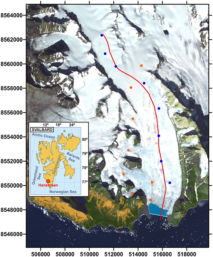
Figure 1. Location of Hansbreen in Spitsbergen, Svalbard (inset). ASTER image of Hansbreen taken in 2011 showing the location of the modeled flowline (red line) and the locations of the stakes for velocity measurements (colored circles; the blue ones were used in this paper). The white triangle indicates the position of Fugleberget Peak. The blue polygon indicates the portion of open water over which the relative coverage of mélange/sea ice was quantified. UTM coordinates for zone 33X are included.

Glacier Geometry

To account for gentle surface slopes, glacier surface elevations were taken from the SPIRIT Digital Elevation Model (DEM) V1 (whose correlation parameters are set for gentle slopes), based on SPOT5 Stereoscopic Survey of Polar Ice imagery acquired on 1 September 2008. The DEM has a 40 m resolution and a 30 m root-mean-square (RMS) absolute horizontal precision (http://polardali.spotimage.fr:8092/wstools/IPY/).

Bed topography was derived from ground-penetrating radar (GPR) data (Grabiec et al., 2012; Navarro et al., 2014) and depth soundings in the glacier forebay (Vieli et al., 2002). The resulting initial geometry of the modeled glacier is shown in Figure 2.

FIGURE 2

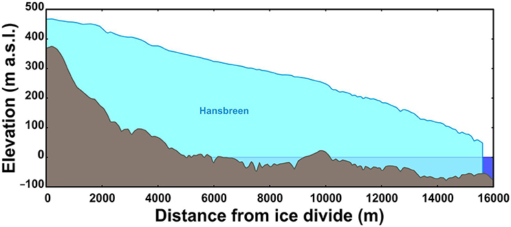
Figure 2. Initial geometry of the modeled flowline representing Hansbreen in September 2008.

Surface Velocity

Surface velocities were measured daily at 16 stakes (Figure 1) between May 2005 and April 2011, using differential GPS (Puczko, 2012). In this study, we focus on a subset of eight stakes close to the modeled flowline (Figure 3). We additionally use velocities of the calving front measured in 2009 by terrestrial laser scanning (TLS; data generously provided by Jacek Jania [University of Silesia] from surveying and data processing by Jacek Krawiec [Laser 3D], Artur Adamek [Warsaw University of Technology], and Jacek Jania). Since a value for the velocity at the calving front is needed at each time step during the entire simulation period, but we only have TLS measurements for 2009, we assume a constant ratio between the frontal velocities and those at the closest stake.

FIGURE 3

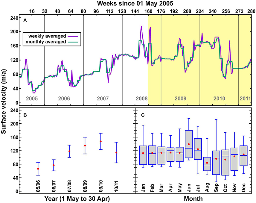
Figure 3. (A) Glacier surface velocities (purple line: weekly averages, green line: monthly averages) measured at the stake closest to the calving front. Yellow highlighting represents the modeled period. (B) Annual means and standard deviations of the glacier surface velocities from 1 May to 30 April the following year. (C) Box-and-whisker plot (computed using Statgraphics ^® centurion) of glacier surface velocities by month for all years (red dots: means, blue interior lines: medians).

The near-terminus surface velocities exhibit a seasonal pattern overlaid by strong interannual variability. Each year has a spring speed up, followed by a rapid slow down, followed sometimes by a gradual speed up through the winter (Figure 3A). In 2005–2006, the highest velocities occurred in summer, while in 2007 the highest velocities occurred in November–December. In 2010, velocities remained very high through winter and spring before dropping dramatically during the summer. In 2008–2011, velocities were much higher than in 2005–2008. The mean varied considerably between years (Figure 3B), discouraging the use of a single mean velocity in the model. Similarly, the very large interannual variability discourages the use of summer and winter means for summer and winter modeled periods (Figure 3C).

Front Positions

Interannual observations of Hansbreen's terminus position over the last decades reveal a generally smooth retreat with occasional abrupt changes (e.g., Vieli et al., 2002). Seasonal variations of the terminus position have also been observed (Blaszczyk et al., 2013). The “weekly” (assuming a week as a 1/48 of a year) terminus positions used in this paper were derived from time-lapse photographs of the Hansbreen terminus taken ca. every 3 h from December 2009 to September 2011 by three different cameras installed at surveyed positions on the eastern slope of Fugleberget (Figure 1). The two Canon EOS 1000D cameras (each equipped with a Canon EF-S 18–55 mm lens) were calibrated from images of a grid pattern using the Camera Calibration Toolbox for Matlab (www.vision.caltech.edu/bouguetj/calib_doc/), while the Canon Powershot A530 camera (which no longer existed at the time of the analysis) had to be calibrated and oriented simultaneously from multiple images of ground control points surveyed by L. Kolondra (unpublished report, 2011). Terminus positions were mapped by tracing the waterline along the terminus in each image, then projecting those pixel coordinates onto a horizontal plane at an altitude of 0 m (tidal heights were not available) to convert them to world coordinates. Standard errors of 0.47 m in water level due to tides (Zagórski et al., 2015; Michał Ciepły, personal communication, 2012), 0.68 pixels due to uncertainties in terminus tracing, and 3.23, 5.70, and 10.53 pixels for each of the three cameras due to uncertainties in camera calibration and orientation result in standard errors for width-averaged glacier length of 3.79, 3.37, and 14.54 m, respectively.

Ice Mélange

The ice mélange in the glacier forebay was qualitatively evaluated as either “complete,” “partial,” or “free” from the same time-lapse photographs used to measure terminus position. For the remaining period, we used the values of the nearest cell in a 25-km resolution time series of sea ice concentrations derived from Nimbus-7 SMMR and DMSP SSM/I-SSMIS passive microwave data (Cavalieri, 1996, updated yearly). These values were used taking into account the partial overlap of the grid cell with Hornsund fjord mouth, and their comparable sizes (Figure 4).

FIGURE 4

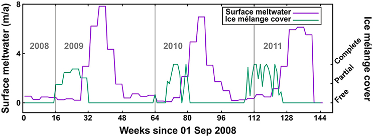
Figure 4. Modeled surface meltwater near the calving front (purple line) and observed ice mélange coverage (weekly average of daily observations) in the glacier forebay (green). Week means here 1/48 of a year.

Surface Mass Balance and Surface Meltwater

We apply a dynamical downscaling method (which uses a modified version of the Polar WRF 3.4.1 model) to produce—from a regional climate dataset consisting of meteorological, sea-surface temperature and sea-ice concentration data—input data for glacier thermomechanical modeling of Hansbreen (Finkelnburg et al., in preparation).

Surface mass balance (SMB) was obtained from European Arctic Reanalysis (EAR) data, with 2 km horizontal resolution and hourly temporal resolution, constrained by automatic weather stations (one in Hornsund and two in Hansbreen) and stake observations (Finkelnburg, 2013). First, ablation was calculated from the surface energy balance (SEB), which is resolved in the EAR by an optimized version of the unified NOAA Land Surface Model (Chen and Dudhia, 2001) of the Polar WRF 3.4.1 model. The algorithm solving for the SEB takes into account net radiation, sensible heat flux, latent heat flux, and ground heat flux, and encompasses all heat fluxes involved in melt and refreezing processes within the snowpack. Second, accumulation was obtained as the solid (frozen) precipitation of the Morrison bulk microphysics scheme for cloud physics used by the EAR. Finally, monthly mean SMB and surface meltwater (SMW) at each flowline point was calculated by applying bilinear interpolation to the available 2-km resolution hourly accumulation and ablation data (Figure 4).

Model Description

Dynamical Model Equations and Flow Law

Ice is treated as an incompressible viscous fluid. The Stokes system of equations describing the dynamical model is composed of equations describing the steady conservation of linear momentum and the conservation of mass of an incompressible continuous medium:

$\begin{array}{rc}div(\sigma )+\rho \text{g}+\text{f}=0,& (1)\end{array}$

$\begin{array}{r}div(\text{u})=0,\end{array}$

where σ is the Cauchy stress tensor, u is the velocity vector, g is the gravity force vector and ρ is the density. The body force f is added to account, in our 2-dimensional (2-D) model, for the friction on the lateral side of the glacier. To this end, the concept of shape factor (Nye, 1965) is here extended to the full-Stokes formulation by defining the body force f as (Jay-Allemand et al., 2011):

$\begin{array}{rc}\text{f}=-\rho \text{g}·\text{t}(1-f)\text{t},& (2)\end{array}$

where the shape factor f = f(x) is a scalar function of the transversal shape of the glacier and t is the unit vector tangent to the upper surface. Jay-Allemand et al. (2011) evaluated f(x) by assuming that the transverse shape of the bedrock is a parabola, and they found an empirical estimate of the shape factor:

$\begin{array}{rc}f=\frac{2}{\pi }{tan}^{-1}\left(\frac{0.186w}{h}\right),& (3)\end{array}$

where h(x) = z_s(x)−b(x) is the ice thickness (expressed as the difference between the surface and bed elevations) and w(x) is the half-width at the glacier surface.

As the constitutive relation, we adopt Nye's generalization of Glen's flow law (Glen, 1955; Nye, 1957):

$\begin{array}{rc}\tau =2\eta \dot{\epsilon }& (4)\end{array}$

This equation links the deviatoric stress τ to the strain rate $\dot{\epsilon }$. The effective viscosity η is written as

$\begin{array}{rc}\eta =\frac{1}{2}{(EA)}^{-1/n}{\text{I}}_{{\dot{\epsilon }}_2}^{(1-n)/n},& (5)\end{array}$

where ${\text{I}}_{{\dot{\epsilon }}_2}^2$ represents the square of the second invariant of the strain rate tensor, A is the softness parameter in Glen's flow law and E is an enhancement factor.

The constitutive relation (4) is expressed in terms of deviatoric stresses, while the conservation of linear momentum (1) is given in terms of full (Cauchy) stresses. Both stresses are linked through the equation

$\begin{array}{rc}\sigma =\tau -p\text{I},p=-tr(\sigma )/3,& (6)\end{array}$

where p is the pressure (compressive mean stress). Typical values for the flow-law exponent (n = 3) and softness (A = 0.1 bar⁻³a⁻¹) were used in the model (Albrecht et al., 2000; Vieli et al., 2002). This value of softness is adequate (see e.g., Cuffey and Paterson, 2010) for a polythermal glacier like Hansbreen, composed mostly of temperate ice except for a thin upper layer of cold ice in the ablation zone (Jania et al., 1996).

Continuum Damage Mechanics Model

We introduce a scalar damage variable D that quantifies the loss of load-bearing surface area due to fractures, known as fracture-induced softening (Borstad et al., 2012). This softening is taken into account through the introduction of the damage within Glen's law. Following Borstad et al. (2012) and Krug et al. (2014), the enhancement factor E can be linked to the damage D as

$\begin{array}{rc}E=\frac{1}{{(1-D)}^n}& (7)\end{array}$

For undamaged ice (D = 0), E = 1 and the flow regime is unchanged. As damage increases (D > 0), E > 1, ice viscosity decreases, and flow velocity increases.

In this study, we use a very simple function for D. Damage is nonzero only in the lowermost 2 km of the glacier (near-terminus heavily crevassed area) and increases linearly toward the terminus, where it reaches a maximum value of 0.4 (Krug et al., 2015). This value provided a good fit to observed velocities in preliminary experiments (not shown here) of the sensitivity of the modeled velocities to changes in damage.

Free Surface Evolution

The time evolution of the glacier surface is calculated by solving the free-surface evolution equation

$\begin{array}{rc}\frac{\partial z_S}{\partial t}=b-u_S\frac{\partial z_S}{\partial x}+v_S,& (8)\end{array}$

where z_S is the surface elevation, t is time, u_S and v_S are the horizontal and vertical components of the flow velocity at the surface, respectively, and b is the surface mass balance.

Boundary Conditions

The upper surface of the glacier is a traction-free zone with unconstrained velocities. At the ice divide at the head of the glacier, horizontal velocity and shear stresses are set to zero.

For boundary conditions at the bed, we use a friction law that relates the sliding velocity to the basal shear stress in such a way that the latter is not set as an external condition but part of the solution:

$\begin{array}{rc}C{u}_t={\sigma }_{nt}& (9)\end{array}$

where C, the friction coefficient, is determined using the inverse Robin method proposed by Arthern and Gudmundsson (2010) and modified by Jay-Allemand et al. (2011). The latter study includes a regularization parameter, λ, for which we have adopted a value of 0.4 determined from preliminary tests. The inverse method infers the basal friction parameter by reducing the mismatch between observed and modeled surface velocities using a cost function.

Since the inversion procedure requires a continuous function for the surface velocity, we calculate it as a sixth-degree polynomial regression for each 4-week period.

At the glacier terminus, we set backstress to zero above sea level and equal to the water-depth-dependent hydrostatic pressure below sea level. In model runs with ice mélange, the additional backstress is applied to the calving face, in the opposite direction of ice flow (negative X). In the absence of further data, we assumed the range of 30–60 kPa estimated by Walter et al. (2012) for Store Gletscher as indicative of the order of magnitude that we could expect for Hansbreen, despite their different settings. While Store Gletscher is buttressed by a rigid proglacial mélange, with a thickness reaching 75 m (Todd and Christoffersen, 2014), Hansbreen presents a thinner layer of ice mélange made up of a mixture of growlers, bergy bits and small icebergs bonded by sea ice. As no measurements of ice mélange thickness in Hansbreen forebay are available, but the sea-ice maximum thickness in Hornsund fjord is known to be around 1 m (Kruszewski, 2012), we assume a mean ice mélange freeboard height of 0.5 m and a mean thickness of 4.5 m.

Calving Model

The CDw calving criterion (Benn et al., 2007) assumes that calving is triggered by the downward propagation of transverse surface crevasses near the calving front as a result of the extensional stress regime. Following Nye (1957), crevasse depth is calculated as the depth where the longitudinal tensile strain rate tending to open the crevasse equals the creep closure resulting from the ice overburden pressure. This procedure incorporates the full stress solution into the crevasse depth criterion. In Benn's model, calving is assumed to occur when surface crevasses reach the waterline.

Following Todd and Christoffersen (2014), crevasse depths are calculated from the balance of forces:

$\begin{array}{rc}{\sigma }_n=2{\tau }_{e}sgn({\tau }_{xx})-{\rho }_{i}gd+P_w& (10)\end{array}$

where σ_n, the “net stress,” is positive for extension and negative for compression. The first term on the right-hand side of Equation (10) represents the opening force of longitudinal stretching, adapted by Todd and Christoffersen (2014) from Otero et al. (2010); τ_e represents the effective stress, ${\tau }_e^2={\tau }_{xx}^2+{\tau }_{zx}^2$. τ_e is multiplied by the sign function of the longitudinal deviatoric stress, τ_xx, to ensure that crevasse opening is only produced under longitudinal extension (τ_xx > 0). The second term on the right-hand side is the ice overburden pressure, which leads to creep closure, where ρ_i is the density of glacier ice, g is the acceleration of gravity and d is the crevasse depth. The last term represents the water pressure which contributes to open the crevasse, which is a function of the depth of water filling the crevasse.

Numerical Solution

At each time step, the glacier is divided into a rectangular mesh with 10 vertical layers and a horizontal grid size of ca. 50 m in the upper glacier and ca. 25 m near the terminus. The Stokes system of equations (1) is solved by a finite element method using Elmer/Ice and the 2-D stress and velocity fields are computed along the central flowline (Figure 1). The new surface elevations are computed from the surface mass-balance input and the solved surface velocities using the free-surface evolution equation and the grid nodes are shifted vertically to fit the new geometry.

At the terminus, the grid nodes are shifted down-glacier according to the velocity vector and the length of the time step and the terminus position is updated according to the calving criterion.

Prognostic model runs were carried out with a 1-week (1/48 of a year) time step, starting from the 2008 glacier geometry. Every 4 weeks (four time steps), we ran an initialization process which consisted of solving the Robin problem (Jay-Allemand et al., 2011) to force a best-fit friction coefficient to be used for those four model runs. This forcing was done to minimize the misfit between the observed and modeled velocities. The choice of the initialization time step was made as a compromise between the time resolution needed for capturing the sudden changes in velocity and an acceptable computational cost.

Numerical Experiments and their Results

Our aim was to investigate the influence of ice mélange backstress and crevasse water depth on terminus position. Given the absence of field measurements, we parameterized crevasse water depth in terms of surface meltwater.

First, we analyzed the effect of crevasse water depth held fixed throughout the entire modeled period. Under this scenario, it was not possible to replicate the observed terminus position variations; instead, we constrained the magnitude of the crevasse water depth to that which best approximates the observed terminus positions. Using this best-fit crevasse water depth, we ran a similar sensitivity analysis for ice mélange backstress and determined the backstress that best fits the observed terminus positions. Finally, using this best-fit ice mélange backstress, we ran the model with a time-varying crevasse water depth d_w expressed as a linear function of the surface meltwater M_w (units meters per week) predicted by the SEB model, i.e., d_w = k M_w, where k is a tuning coefficient.

This experiment was repeated for a range of values for the linear coefficient, and the results corresponding to the best-fitting value very closely matched the observed terminus position variations.

Crevasse Water Depth

Given the difficulties of measuring the depth of water in crevasses, we ran the model for a range of crevasse water depths (from 6 to 12 m) to evaluate the sensitivity of the model to this parameter. We found that calving rate is highly dependent on the depth of water in crevasses, with an increase of just a few meters causing the glacier to switch from advance to retreat (Figure 5). If a constant water depth is prescribed, the model is unable to reproduce the observed terminus position fluctuations (Figure 5), although the results allow us to select the water depth which, on average, best fits the observations (10 m, as illustrated by Figure 5).

FIGURE 5

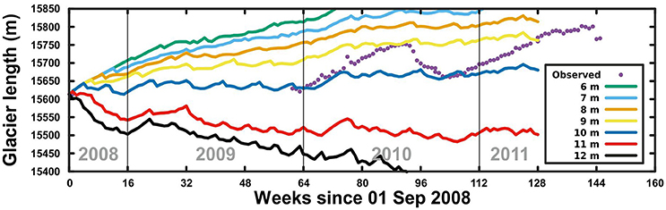
Figure 5. Modeled flowline glacier length for different constant crevasse water depths, with an ice mélange backstress of 50 kPa. Magenta dots represent the observed glacier lengths. Week means here 1/48 of a year.

Ice Mélange

To test the effect of ice mélange on calving rate and terminus position, we varied ice mélange backstress from 0 to 70 kPa (based on Walter et al., 2012, as discussed in the Introduction) in steps of 10 kPa and multiplied by the fraction of ice mélange coverage (weekly average) in the glacier forebay, varying from 0 when no ice mélange is present to 1 when ice mélange completely fills the glacier forebay. When there is only partial coverage of ice mélange, ice mélange remains concentrated near the margins of the glacier and the fjord and therefore continues to exert some backstress on the glacier front. This supports the prescription of backstress even at low ice mélange concentrations. In this experiment, we prescribed a constant crevasse water depth of 10 m, the best-fit value from the previous experiment.

We found that the effect of ice mélange backstress on glacier front position was significant, even under low stresses (Figure 6), and that 50 kPa (for full mélange coverage), applied to the front of the glacier, yielded the best fit to observations during the winter when ice mélange was present. The effect of a backstress of 50 kPa on the modeled longitudinal deviatoric stress profile is shown in Figure 7.

FIGURE 6

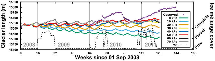
Figure 6. Modeled flowline glacier length for different constant values of ice mélange backstress, with a constant crevasse water depth of 10 m. Magenta dots represent the observed glacier lengths. The dashed line indicates the observed ice mélange coverage (IMC) in the glacier forebay. Week means here 1/48 of a year.

FIGURE 7

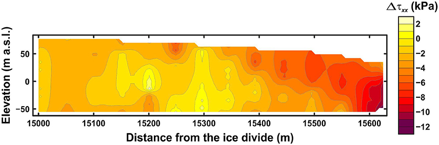
Figure 7. Change in longitudinal deviatoric stress, in the terminal part of the glacier, resulting from an increase in ice mélange backstress from 0 to 50 kPa at the calving front.

Surface Meltwater

As discussed by Todd and Christoffersen (2014), the relationship between surface melt rate and crevasse water depth depends on many factors, including the distribution, shape, and depth of crevasses, the melting and refreezing on crevasse walls, and the potential drainage of water from crevasses into englacial, subglacial, and proglacial water bodies. Since observations of these processes are very scarce and the water in crevasses starts as surface meltwater, we chose to parameterize crevasse water depth in terms of the available surface meltwater predicted by the SEB model (Figure 8).

FIGURE 8

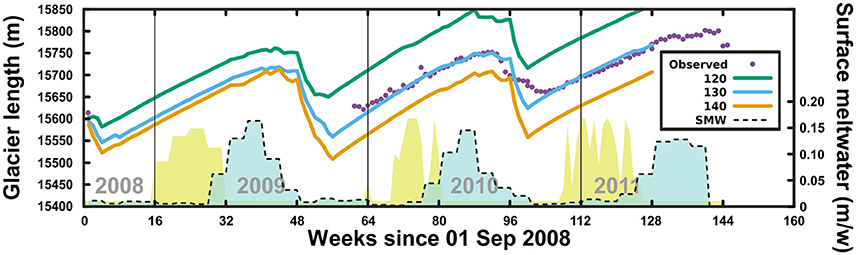
Figure 8. Modeled glacier length for crevasse water depths parameterized as a linear function of the available surface meltwater for a range of values of the linear coefficient k (shown in box), with an ice mélange backstress of 50 kPa. Magenta dots represent the observed glacier lengths. The dashed line indicates the modeled surface meltwater near the calving front. Yellow shaded areas represent the observed ice mélange coverage in the glacier forebay. Week means here 1/48 of a year.

Use of such a parameterized time-varying crevasse water depth, in combination with the best-fit ice mélange backstress from the previous experiment, yielded terminus positions in very good agreement with the observations (Figure 8), reproducing the winter advance and the subsequent summer retreat.

Discussion

In tidewater glacier modeling, it is common practice to use mean annual surface velocities (e.g., Cook et al., 2012, 2014) or seasonal means (e.g., Vieli et al., 2002; Todd and Christoffersen, 2014) to tune the free parameters of the model. In this study, we use a 4-week mean of daily velocity observations to infer a sliding parameter for each 4-week period, with the aim of obtaining more realistic modeled velocities and, consequently, a more realistic calving rate. An accurate representation of velocities is key to glacier models which use a crevasse-depth calving criterion, since such a calving criterion relies on the stress field derived from the velocity field and its associated strains. In particular, higher temporal resolutions for velocities and other model parameters are necessary to capture speed-up events such as those observed at Hansbreen (Figure 3A). Because of the short duration of these events, they have a negligible effect on mean annual and seasonal velocities, but have a significant impact on the stress regime and therefore the calving rate.

Our results demonstrate that our model is capable of reproducing the seasonal fluctuations of the terminus position of Hansbreen, provided that the key model variables are adequately tuned and parameterized.

The modeled terminus positions are shown to be highly sensitive to changes in crevasse water depth, in agreement with previous studies (e.g., Cook et al., 2012). In particular, we found that a small change in depth, from 10 to 11 m, resulted in a switch from advance to retreat (Figure 5). As small changes to parameter values can lead to large changes in the model results (i.e., a mathematical instability), extreme care should be taken when implementing crevasse-depth criteria in prognostic models. Besides, when a constant crevasse water depth is applied the results show a several-month periodicity (Figures 5, 6). This is a consequence of the CDw criterion, as at each time step the glacier terminal zone thins by ablation until the threshold for calving is reached, and then process restarts.

The water in crevasses is mostly produced by melting at the glacier surface, so the mean water depth in crevasses can be parameterized in terms of surface melting, which can be modeled either using air temperature or temperature-radiation index models (e.g., Jonsell et al., 2012) or energy-balance models (e.g., Hock and Holmgren, 2005) trained by observed and/or modeled data (e.g., Finkelnburg, 2013). This allows us to replace a parameter inherently difficult to measure in the field by another that can be based on easier field observations, models, or both.

In contrast with one previous modeling study (Cook et al., 2014), but in agreement with another (Todd and Christoffersen, 2014), our results suggest that ice mélange backstress is an important control on calving and should not be ignored. A change from 0 to 50 kPa in backstress resulted in a change of ca. 170 m in glacier length over 2.5 years (Figure 6). In addition, our simulations show how the presence of ice mélange may prevent calving, as others have established from observations (Amundson et al., 2010; Howat et al., 2010). When a backstress of 50 kPa of ice mélange is present, the glacier advances but does not calve. Therefore, any higher backstress (up to 70 kPa) has no further effect on calving and has only a very minor effect on front position. Calving, accompanied by ice front retreat, is only occasionally produced during the warmer periods, in absence of ice mélange.

Both our model and the observations show frontal retreat beginning soon after the peak in surface meltwater, although the maximum calving occurs a few weeks later, suggesting a delayed response by the glacier system to meltwater input. The source of this lag could be two-fold. On one hand the cumulative effect of thinning by ablation in both the real glacier and the model, which helps the crevasses to penetrate down to the waterline. On the other hand, in the case of the real glacier there is a buildup of the water pressure in the crevasses as meltwater accumulates; alternatively, if the water escapes from the crevasses there will also be a cumulative weakening of the bulk of the terminal zone of the glacier due to the enlargement of the conduits and fissures by melting promoted by the escaping water.

Even though our model does a good job reproducing the observed front positions, it does not consider other possible controls on the calving process, specifically ocean-induced melting. Adequately incorporating this mechanism would require developing a fjord circulation model to estimate the subaqueous melt rates and couple the fjord and glacier systems.

In regards to possible shortcomings of the model, we note that we added a body force term to the Stokes system (Equation 1) to take into account, in our 2-D flowline model, of the lateral drag on the glacier sidewalls. However, this body force term does not take into consideration the effect of ice flow from tributaries on the central flowline dynamics. This effect is expected to be significant at Hansbreen, which has three tributary glaciers flowing into the main branch near the terminus (Figure 1). To properly model the lateral drag, and take into account the tributary glaciers, a 3-D model would be necessary.

Conclusions

In this study, we investigate the relative importance of some proposed controls on calving—namely, crevasse water depth and ice mélange backstress—and evaluate their influence on the terminus position changes of a tidewater glacier.

Our results suggest that ice mélange backstress plays an important role in regulating the seasonal advance and retreat of the terminus, mostly by preventing calving when the mélange chokes the fjord. The model results also indicate that calving and the associated terminus position changes are highly sensitive to the amount of water filling near-terminus crevasses, itself a function of surface meltwater availability. The sensitivity of calving rate to crevasse water depth suggests that calving is strongly affected by atmospheric forcing. These results, taken together, show that tidewater glacier dynamics are influenced by both oceanic and atmospheric processes, and that neither of them should be ignored.

Author Contributions

JO led the study. JO and FN designed the experiments. JO did the numerical modeling of glacier dynamics and RF provided regional climate modeling and SEB data. JL provided GPR data, DP ice velocity and AWS data, and EW terminus positions and sea ice coverage data. JO, FN, and JL contributed to the discussion of the results. JO and FN wrote the initial draft of the paper primarily, JL made the figures. All authors contributed to and approved the final manuscript.

Funding

This research was funded by Spanish State Plan for Research and Development (R&D) project CTM2014-56473-R. Field data collection was funded by grants EUI2009-04096 and CTM2011-28980 of the Spanish Programmes of Euro-Research and R&D, respectively, and the Polish National Science Centre within statutory activities No3841/E-41/S/2014 of the Ministry of Science and Higher Education of Poland. The regional climate modeling data was produced under grant no. SCHE 750/3-1 of the German Research Foundation (DFG) and grant no. 03F0623A of the German Federal Ministry of Education and Research (BMBF).

Conflict of Interest Statement

The authors declare that the research was conducted in the absence of any commercial or financial relationships that could be construed as a potential conflict of interest.

Acknowledgments

This research was carried out under the frames of the International Arctic Science Committee Network on Arctic Glaciology (IASC-NAG) and the European Science Foundation PolarCLIMATE programme's SvalGlac project. The satellite images used in this paper were provided by the SPIRIT Program CNES (2008), Spot Image, and ASTER METI and NASA (2011), all rights reserved. The surface velocity data used in the paper were collected based on Stanislaw Siedlecki Polish Polar Station in Hornsund.

References

Albrecht, O., Jansson, P., and Blatter, H. (2000). Modelling glacier response to measured mass-balance forcing. Ann. Glaciol. 31, 91–96. doi: 10.3189/172756400781819996

CrossRef Full Text | Google Scholar

Amundson, J. M., Fahnestock, M., Truffer, M., Brown, J., Lüthi, M. P., and Motyka, R. J. (2010). Ice mélange dynamics and implications for terminus stability, Jakobshavn Isbræ, Greenland. J. Geophys. Res. 115:F01005. doi: 10.1029/2009JF001405

CrossRef Full Text | Google Scholar

Amundson, J. M., and Truffer, M. (2010). A unifying framework for iceberg-calving models. J. Glaciol. 56, 822–830. doi: 10.3189/002214310794457173

CrossRef Full Text | Google Scholar

Arthern, R., and Gudmundsson, G. (2010). Initialization of ice-sheet forecasts viewed as an inverse Robin problem, J. Glaciol. 56, 527–533. doi: 10.3189/002214310792447699

CrossRef Full Text | Google Scholar

Bassis, J. N. (2011). The statistical physics of iceberg calving and the emergence of universal calving laws. J. Glaciol. 57, 3–16. doi: 10.3189/002214311795306745

CrossRef Full Text | Google Scholar

Benn, D. I., and Evans, D. J. A. (2010). Glaciers and Glaciation, 2nd Edn. London; New York, NY: Hodder Education.

Benn, D. I., Hulton, N. R. J., and Mottram, R. H. (2007). ≪Calving laws≫, ≪sliding laws≫ and the stability of tidewater glaciers. Ann. Glaciol. 46, 123–130. doi: 10.3189/172756407782871161

CrossRef Full Text | Google Scholar

Blaszczyk, M., Jania, J. A., and Kolondra, L. (2013). Fluctuations of tidewater glaciers in Hornsund Fjord (Southern Svalbard) since the beginning of the 20 th century. Polish Polar Res. 34, 327–352. doi: 10.2478/popore-2013-0024

CrossRef Full Text | Google Scholar

Bondzio, J. H., Seroussi, H., Morlighem, M., Kleiner, T., Rückamp, M., Humbert, A., et al. (2016). Modelling calving front dynamics using a level-set method: application to Jakobshavn Isbræ, West Greenland. Cryosphere 10, 497–510. doi: 10.5194/tc-10-497-2016

CrossRef Full Text | Google Scholar

Borstad, C. P., Khazendar, A., Larour, E., Morlighem, M., Rignot, E., Schodlok, M. P., et al. (2012). A damage mechanics assessment of the Larsen B ice shelf prior to collapse: toward a physically-based calving law. Geophys. Res. Lett. 39, L18502. doi: 10.1029/2012gl053317

CrossRef Full Text | Google Scholar

Cavalieri, D. J., Parkinson, C. L., Gloersen, P., and Zwally, H. J. (1996). updated yearly. Sea Ice Concentrations from Nimbus-7 SMMR and DMSP SSM/I-SSMIS Passive Microwave Data, Version 1. Boulder, CO: USA. NASA National Snow and Ice Data Center Distributed Active Archive Center.

Chen, F., and Dudhia, J. (2001). Coupling an advanced land surface-hydrology model with the Penn State-NCAR MM5 Modeling System. Part I: Model Implementation and Sensitivity. Monthly Weather Rev. 129, 569–585. doi: 10.1175/1520-0493(2001)129<0569:CAALSH>2.0.CO;2

CrossRef Full Text | Google Scholar

Cook, S., Rutt, I. C., Murray, T., Luckman, A., Zwinger, T., Selmes, N., et al. (2014). Modelling environmental influences on calving at Helheim Glacier in eastern Greenland. Cryosphere 8, 827–841. doi: 10.5194/tc-8-827-2014

CrossRef Full Text | Google Scholar

Cook, S., Zwinger, T., Rutt, I. C., O'Neel, S., and Murray, T. (2012). Testing the effect of water in crevasses on a physically based calving model. Ann. Glaciol. 53, 90–96. doi: 10.3189/2012AoG60A107

CrossRef Full Text | Google Scholar

Cuffey, K., and Paterson, W. (2010). The Physics of Glaciers. Elsevier, 4th Edn. Oxford: Elsevier.

Google Scholar

Finkelnburg, R. (2013). Climate Variability of Svalbard in the First Decade of the 21st Century and its Impact on Vestfonna ice cap, Nordaustlandet - An Analysis based on Field Observations, Remote Sensing and Numerical Modeling. Doctoral thesis, Technische Universität Berlin. Berlin.

Gagliardini, O., Zwinger, T., Gillet-Chaulet, F., Durand, G., Favier, L., de Fleurian, B., et al. (2013). Capabilities and performance of Elmer/Ice, a new-generation ice sheet model. Geosci. Model Dev. 6, 1299–1318. doi: 10.5194/gmd-6-1299-2013

CrossRef Full Text | Google Scholar

Gardner, A. S., Moholdt, G., Cogley, J. G., Wouters, B., Arendt, A. A., Wahr, J., et al. (2013). A reconciled estimate of glacier contributions to sea level rise: 2003 to 2009. Science 340, 852–857. doi: 10.1126/science.1234532

PubMed Abstract | CrossRef Full Text | Google Scholar

Glen, J. W. (1955). The creep of polycrystalline ice. Proc. R. Soc. Lond. A Math. Phys. Sci. 228, 519–538. doi: 10.1098/rspa.1955.0066

CrossRef Full Text | Google Scholar

Grabiec, M., Jania, J. A., Puczko, D., Kolondra, L., and Budzik, T. (2012). Surface and bed morphology of Hansbreen, a tidewater glacier in Spitsbergen. Polish Polar Res. 33, 111–138. doi: 10.2478/v10183-012-0010-7

CrossRef Full Text | Google Scholar

Hock, R., and Holmgren, B. (2005). A distributed surface energy-balance model for complex topography and its application to Storglaciären, Sweden. J. Glaciol. 51, 25–36. doi: 10.3189/172756505781829566

CrossRef Full Text | Google Scholar

Howat, I. M., Box, J. E., Ahn, Y., Herrington, A., and McFadden, E. M. (2010). Seasonal variability in the dynamics of marine-terminating outlet glaciers in Greenland. J. Glaciol. 56, 601–613. doi: 10.3189/002214310793146232

CrossRef Full Text | Google Scholar

Huss, M., and Hock, R. (2015). A new model for global glacier change and sea-level rise. Front. Earth Sci. 3:54. doi: 10.3389/feart.2015.00054

CrossRef Full Text | Google Scholar

Jania, J., Mochnacki, D., and Gadek, B. (1996). The thermal structure of Hansbreen, a tidewater glacier in southern Spitsbergen, Svalbard. Polar Res. 15, 53–66. doi: 10.3402/polar.v15i1.6636

CrossRef Full Text | Google Scholar

Jay-Allemand, M., Gillet-Chaulet, F., Gagliardini, O., and Nodet, M. (2011). Investigating changes in basal conditions of Variegated Glacier prior to and during its 1982-1983 surge. Cryosphere 5, 659–672. doi: 10.5194/tc-5-659-2011

CrossRef Full Text | Google Scholar

Jonsell, U. Y., Navarro, F. J., Bañón, M., Lapazaran, J. J., and Otero, J. (2012). Sensitivity of a distributed temperature-radiation index melt model based on AWS observations and surface energy balance fluxes, Hurd Peninsula glaciers, Livingston Island, Antarctica. Cryosphere 6, 539–552. doi: 10.5194/tc-6-539-201210.5194/tc-6-539-2012

CrossRef Full Text | Google Scholar

Krug, J., Durand, G., Gagliardini, O., and Weiss, J. (2015). Modelling the impact of submarine frontal melting and ice mélange on glacier dynamics. Cryosphere 9, 989–1003. doi: 10.5194/tc-9-989-2015

CrossRef Full Text | Google Scholar

Krug, J., Weiss, J., Gagliardini, O., and Durand, G. (2014). Combining damage and fracture mechanics to model calving. Cryosphere 8, 2101–2117. doi: 10.5194/tc-8-2101-2014

CrossRef Full Text | Google Scholar

Kruszewski, G. (2012). Zlodzenie Hornsundu i wód przyległych (Spitsbergen) w sezonie zimowym 2010-2011 (Ice conditions in Hornsund and adjacent waters (Spitsbergen) during winter season 2010-2011), Problemy Klimatologii Polarnej 22, 69–82.

Google Scholar

Luckman, A., Benn, D. I., Cottier, F., Bevan, S., Nilsen, F., and Inall, M. (2015). Calving rates at tidewater glaciers vary strongly with ocean temperature. Nat. Commun. 6:8566. doi: 10.1038/ncomms9566

PubMed Abstract | CrossRef Full Text | Google Scholar

Morlighem, M., Bondzio, J., Seroussi, H., Rignot, E., Larour, E., Humbert, A., et al. (2016). Modeling of Store Gletscher's calving dynamics, West Greenland, in response to ocean thermal forcing. Geophys. Res. Lett. 43, 2659–2666. doi: 10.1002/2016GL067695

CrossRef Full Text | Google Scholar

Motyka, R. J. (1997). Deep-water calving at Le Conte Glacier, southeast Alaska. Byrd Polar Res. Cent. Rep. 15, 115–118.

Navarro, F. J., Martín-Español, A., Lapazaran, J. J., Grabiec, M., Otero, J., Vasilenko, E. V., et al. (2014). Ice volume estimates from ground-penetrating radar surveys, Wedel Jarlsberg land glaciers, Svalbard. Arct. Antarct. Alp. Res. 46, 394–406. doi: 10.1657/1938-4246-46.2.394

CrossRef Full Text | Google Scholar

Nick, F. M., van der Veen, C. J., Vieli, A., and Benn, D. I. (2010). A physically based calving model applied to marine outlet glaciers and implications for the glacier dynamics. J. Glaciol. 56, 781–794. doi: 10.3189/002214310794457344

CrossRef Full Text | Google Scholar

Nye, J. F. (1957). The distribution of stress and velocity in glaciers and ice-sheets. Proc. R. Soc. A 239, 113–133. doi: 10.1098/rspa.1957.0026

CrossRef Full Text | Google Scholar

Nye, J. F. (1965). The flow of a glacier in a channel of rectangular, elliptic or parabolic cross-section. J. Glaciol. 5, 661–690. doi: 10.1017/S0022143000018670

CrossRef Full Text | Google Scholar

Oerlemans, J., Jania, J., and Kolondra, L. (2011). Application of a minimal glacier model to Hansbreen, Svalbard. Cryosphere 5, 1–11. doi: 10.5194/tc-5-1-2011

CrossRef Full Text | Google Scholar

Otero, J., Navarro, F. J., Martin, C., Cuadrado, M. L., and Corcuera, M. I. (2010). A three-dimensional calving model: numerical experiments on Johnsons Glacier, Livingston Island, Antarctica. J. Glaciol. 56, 200–214. doi: 10.3189/002214310791968539

CrossRef Full Text | Google Scholar

Petlicki, M., Cieply, M., Jania, J. A., Prominska, A., and Kinnard, C. (2015). Calving of a tidewater glacier driven by melting at the waterline. J. Glaciol. 61, 851–863. doi: 10.3189/2015JoG15J062

CrossRef Full Text | Google Scholar

Puczko, D. (2012). Czasowa I Przestrzenna Zmienność Ruchu Spitsbergeńskich Lodowców Uchodzących Do Morza Na Przykładzie Lodowca Hansa. Temporal And Spatial Variability Of Tidewater Glaciers Movement Based On Example Of Hansbreen. Doctoral thesis, Institute of Geophysics, Polish Academy of Sciences, Warsaw.

Rignot, E., Jacobs, S., Mouginot, J., and Scheuchl, B. (2013). Ice-Shelf Melting Around Antarctica. Science 341, 266–270. doi: 10.1126/science.1235798

PubMed Abstract | CrossRef Full Text | Google Scholar

Scambos, T., Hulbe, C., and Fahnestock, M. (2003), “Climate-induced ice shelf disintegration in the Antarctic Peninsula,” in Antarctic Peninsula Climate Variability: Historical and Paleoenvironmental Perspectives, eds E. Domack, A. Levente, A. Burnet, R. Bindschadler, P. Convey, and M. Kirby (Washington, DC: American Geophysical Union), 79–92. doi: 10.1029/AR079p0079

CrossRef Full Text

Todd, J., and Christoffersen, P. (2014). Are seasonal calving dynamics forced by buttressing from ice mélange or undercutting by melting? Outcomes from full-Stokes simulations of Store Glacier, West Greenland. Cryosphere 8, 2353–2365. doi: 10.5194/tc-8-2353-2014

CrossRef Full Text | Google Scholar

Vieli, A., Jania, J., and Kolondra, L. (2002). The retreat of a tidewater glacier: observations and model calculations on Hansbreen, Spitsbergen. J. Glaciol. 48, 592–600. doi: 10.3189/172756502781831089

CrossRef Full Text | Google Scholar

Walter, J. I., Box, J. E., Tulaczyk, S., Brodsky, E. E., Howat, I. M., Ahn, Y., et al. (2012). Oceanic mechanical forcing of a marine-terminating Greenland glacier. Ann. Glaciol. 53, 181–192. doi: 10.3189/2012AoG60A083

CrossRef Full Text | Google Scholar

Zagórski, P., Rodzik, J., Moskalik, M., Strzelecki, M. C., Lim, M., Błaszczyk, M., et al. (2015). Multidecadal (1960–2011) shoreline changes in Isbjørnhamna (Hornsund, Svalbard). Polish Polar Res. 36, 369–390. doi: 10.1515/popore-2015-0019

CrossRef Full Text | Google Scholar