Hydraulic Conductivity of a Firn Aquifer in Southeast Greenland

Introduction

Across the percolation zone of the southeast portion of the Greenland ice sheet, surface meltwater infiltrates to depth within the ice sheet, where it currently forms an extensive firn aquifer. The firn aquifer contains liquid water within the pore space of the compacting snow/firn throughout the year at depths of ~10–30 m. Initially documented in 2011 (Forster et al., 2014), the aquifer has been identified and monitored with ground penetrating radar, airborne radar, and in situ measurements since then (Koenig et al., 2014; Miège et al., 2016; Montgomery et al., this issue). Over the entire ice sheet, firn aquifers are estimated to cover an area between 20,000 and 70,000 km², with ~50% of this total extent located in the southeastern portion of the ice sheet (Forster et al., 2014; Miège et al., 2016). Firn aquifers form in areas with a combination of high accumulation and high melt rates (Forster et al., 2014; Kuipers Munneke et al., 2014). Complete drainage of the aquifer could contribute up to 0.4 mm to sea level rise globally (Koenig et al., 2014).

In a firn aquifer, water storage occurs as meltwater fills firn pore space until the residual liquid water content of the firn is achieved, which allows horizontal flow to occur (Freeze and Cherry, 1979; Pfeffer et al., 1991). Water flow within the firn aquifer may allow surface meltwater originating far from the edge of the ice sheet to discharge to the ocean. The saturation of the firn allows more meltwater that would otherwise rest in pore spaces if the firn remained unsaturated to flow laterally. Crevasses at the edge of the ice sheet represent one possible pathway for aquifer water to discharge to the ocean (Alley et al., 2005; Chu, 2014; Koenig et al., 2014). Transport of liquid water to the base of the ice sheet, likely via crevasses (Miège et al., 2016; Poinar et al., 2017) may also influence ice dynamics and ice discharge to the ocean (e.g., Zwally, 2002; Joughin et al., 2008; Sole et al., 2011). The hydrologic properties of the aquifer and its connections to the broader glacier hydrologic system remain unclear. The aquifer may be storing meltwater and buffering sea level rise, or it may be constantly draining and routing water toward the ocean. To characterize the connection between surface melt and discharge to the ocean, and quantify water flow, hydraulic properties of the aquifer are required.

This process of water storage and transport differs from meltwater discharge to the ocean in other parts of Greenland, where inland meltwater is routed through surface lakes and streams to crevasses and moulins (Das et al., 2008; Lewis and Smith, 2009; Chu, 2014; Smith et al., 2015). In some areas outside of firn aquifer regions, thick ice layers prevent meltwater percolation to depth and surface runoff is favored, contributing to sea level rise (Machguth et al., 2016). In other areas, meltwater storage occurs by refreezing in the firn, buffering sea level rise (Pfeffer et al., 1991; Harper et al., 2012).

The storage and transmission of meltwater through firn is similar in many ways to water flow through a rocky or unconsolidated porous media, where water flows from recharge to discharge areas (high hydraulic head to low hydraulic head). The undulating water table observed in radar profiles (Forster et al., 2014) resembles the topographically driven flow of an unconfined aquifer (Tóth, 1963). In the unsaturated zone above the water table, where fluid pressures are less than atmospheric, pores can contain both gas and liquid. The aquifer is defined as the saturated zone below the water table, where fluid pressures are positive. Isolated gas phases within the saturated zone can exist. We conceptualize saturated groundwater flow to follow Darcy's law:

$\begin{array}{ll}q=\frac{Q}{A}=-K\frac{\partial h}{\partial x}& (1)\end{array}$

where q is the specific discharge (length/time), Q is the discharge (length³/time), A is the cross sectional area across which flow occurs (length²), K is the hydraulic conductivity (length/time), h is the hydraulic head (length), and x is the distance (length). To quantify aquifer discharge, the hydraulic gradient can be estimated from ground penetrating radar surveys of the aquifer but site-specific in-situ measurements of hydraulic conductivity are needed.

Hydraulic conductivity is typically measured in situ by two major techniques: aquifer tests and piezometer tests (Freeze and Cherry, 1979). Each test introduces a different hydraulic stress to the system. Aquifer tests involve injecting or pumping water from or into an aquifer at a controlled rate and observing the change in water level over time. Slug tests, a type of piezometer test, involve instantaneously changing the hydraulic head within a well and recording recovery in that well over time (Hvorslev, 1951; Butler, 1997). Both tests induce horizontal flow within the aquifer, and therefore indicate horizontal hydraulic conductivity. Slug tests can provide depth-specific measurements of hydraulic conductivity within a formation. However, the conditions immediately surrounding the piezometer have a larger influence on slug test results.

Aquifer tests assess the hydraulic properties, including hydraulic conductivity, of an aquifer over a larger area (~m–km) than slug tests because they perturb a larger volume of water over a longer period of time (Ferris et al., 1962). Thus, aquifer tests are less subject to formation disturbance caused by the drilling or melting processes that may alter hydraulic conductivity close to the borehole or piezometer. As a result, aquifer tests generally provide a better estimate of the effective hydraulic parameters of an aquifer than slug tests. However, they are technically more difficult to conduct, require more equipment, and take longer than slug tests. The water level response during the recovery period of an aquifer test can provide the most accurate estimate of hydraulic conductivity as it is generally independent of well construction or pumping effects. A comparison of slug and aquifer test results, as is presented in this manuscript, can provide a comprehensive estimate of the hydraulic conductivity within an aquifer.

Firn aquifers have been observed in mountain glaciers, and their hydraulic conductivities have been measured using slug tests and aquifer tests (Oerter and Moser, 1982; Oerter et al., 1983; Fountain, 1989; Fountain and Walder, 1998; Schneider, 1999; Jansson et al., 2003). Slug tests have also been used to estimate subglacial hydraulic properties (Stone and Clark, 1972; Iken et al., 1996; Kulessa et al., 2005; Meierbachtol et al., 2008). Hydraulic conductivity depends on properties of both the porous media (grain size, shape, distribution, and packing) and the fluid (viscosity and density). Firn permeability, which only depends on porous media properties, has been measured at various sites across Greenland using permeameters (Albert and Shultz, 2002; Adolph and Albert, 2014; Keegan et al., 2014) and Antarctica (Albert et al., 2000, 2004). Hydraulic conductivity (K) is related to permeability (k) as

$\begin{array}{ll}K=\frac{k\rho g}{\mu }& (2)\end{array}$

where ρ is fluid density, g is the acceleration due to gravity, and μ is the fluid dynamic viscosity. These parameters can shed light on the depositional and metamorphic history of the firn.

In this manuscript, we describe the methods and results of field experiments conducted to determine, for the first time, the hydraulic conductivity of a firn aquifer in the southeastern area of the Greenland ice sheet. Mathematical solutions to determine hydraulic conductivity involve matching curves to water displacement data. These results, combined with aquifer geometry, are essential to developing a hydrologic model of the firn aquifer and understanding the impact of the aquifer on ice sheet mass balance estimates.

Materials and Methods

Site Description

The study site is located along an elevation gradient of an ice flow line upstream of Helheim Glacier in southeast Greenland (Figure 1). Field work was conducted ~40 km west of the glacier front in April, July, and August 2015, and July and August 2016. Five 6.4 cm diameter boreholes were drilled with an electrothermal drill to ~50 m depth, and a heated piezometer, described in Section Heated Piezometer, was installed at 6 sites (Table 1) to a maximum depth of almost 40 m. At two of those drilling sites, piezometers were installed <5 m away from the borehole to perform aquifer tests. The 6.4 cm diameter holes were enlarged with a heated reamer to 8 cm diameter in order to accommodate the pump inside the borehole.

FIGURE 1

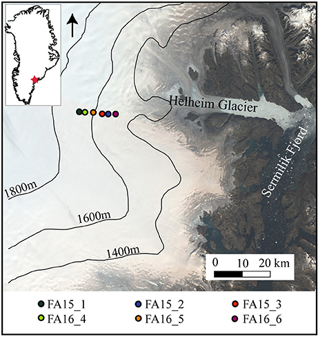
Figure 1. Site map. Landsat 8 composite image (August 21, 2014) showing sites in southeast Greenland where slug tests and aquifer tests were conducted in April, July, and August 2015 and July and August, 2016. Elevation contours from Cryosat-2 DEM (Helm et al., 2014).

TABLE 1

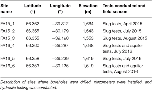
Table 1. Site locations.

We determined the thickness of the aquifer using in-situ and geophysical methods. We measured the depth to the water table with both a chalked steel tape (Garber and Koopman, 1968) and ground penetrating radar (Forster et al., 2014; Miège et al., 2016). We also determined the bottom of the aquifer with a borehole dilution test. Briefly, during the borehole dilution test, we mixed a small amount of saltwater into the 8 cm diameter borehole and measured the specific conductance of the water within the borehole at 30 cm intervals over ~20 h. The reduction in specific conductance due to inflow of freshwater is proportional to the specific discharge through the borehole. Within the aquifer, the change in specific discharge was significant, but below a certain depth, the specific discharge did not change, indicating the bottom of the flow zone. We only did this test in 2016. The other method to determine the bottom of the aquifer is with a seismic survey, described in Montgomery et al. this issue. The depth to the water table and aquifer bottom and aquifer thickness using each method at each site are shown in Table 2. The thickness of the saturated zone determined by the borehole dilution test was used where available. The seismic bottom depths were also used. The borehole dilution and seismic thicknesses do not perfectly agree (5–17 m differences) and so a range of thicknesses were used for the hydraulic conductivity estimates.

TABLE 2

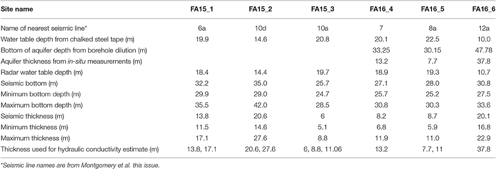
Table 2. Depth to water table and aquifer bottom, and aquifer thickness measurements from in-situ and geophysical methods.

Heated Piezometer

A piezometer, commonly used in groundwater hydrology, consists of a sealed pipe with an open end installed in the porous media to measure depth-specific hydraulic heads. We adapted a piezometer to penetrate the numerous ice lenses within the firn through the addition of a heated tip that allows the piezometer to advance by melting through the firn and ice (Figure 2). The 3 cm diameter piezometer standpipe is closed along its entire length except for a 32 cm screened interval near the tip which allows water to enter or exit when advanced below the water table. The casing radius is 1.5 cm, and the well radius is 1.5 cm. The piezometer also features a 108 cm long packer made of rubber surgical tubing, which can be inflated from the surface and allows for depth-specific measurements and water sampling. A generator at the surface powers the 500 W heated tip. A power cable and hollow tube to inflate the packer run from the surface to the heated tip and packer along the inside of the metal pipe above the packer. A bicycle pump is used to inflate the packer, which surrounds a section of the metal pipe above the screened interval, to a pressure of ~1.7 atm (25 psi) above the water pressure.

FIGURE 2

Figure 2. The heated piezometer. Diagram (A) and photo (B) of the heated piezometer. The piezometer, consisting of a sealed pipe above an inflatable packer, screened interval, and heated tip at depth, advances to greater depth as the heated tip melts through the firn and ice lenses. Lengths of threaded pipe can be added at the surface as the tip moves downward. A power cable and hollow tube run the length of the pipe to power the heater and allow for packer inflation from the surface. Tubing can be lowered into the piezometer to collect water samples. The screened interval allows for hydraulic testing and water sampling from the entire thickness of firn/ice that the screened interval is open to.

As the piezometer melts through the firn, additional lengths (1.5 m) of threaded pipe are added at the surface. The pipe allows the creation of a sealed volume required to accumulate enough pressure to displace water during the slug tests. The walls of the piezometer were flush to the firn. The piezometer advances at a rate of ~13 cm/min in firn with a density below ~600 kg/m³ and ~3 cm/min in firn and ice above a density of ~600 kg/m³. We advanced the piezometer to a maximum depth of 38 m, limited by the length of pipe available in the field, but in concept could go deeper. The temperature at the maximum piezometer depth was 0°C (±0.2°C), from borehole temperature sensors. Although, never encountered, firn or ice temperatures below 0°C could cause the piezometer to freeze into the ice.

We removed the piezometer with a tripod equipped with a hand winch. The pipe can be pulled out by hand, but can be heavy enough that the tripod pulley system is safer. The piezometer standpipes were commercially available while the tip and packer were custom fabricated. Prior to use on the Greenland ice sheet, the piezometer was tested in ice blocks and on a frozen lake.

Slug Tests

Slug tests are widely used to determine hydraulic conductivity in the saturated zone (Kruseman et al., 1994). During a slug test, water within a piezometer is displaced, and the recovery, which depends on the hydraulic properties of the aquifer, is recorded (Figure 3). These tests are made depth-specific when a seal is formed between the screened interval of the piezometer and the porous media above.

FIGURE 3

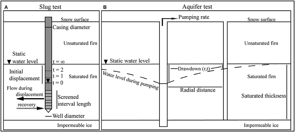
Figure 3. Diagrams of slug and aquifer tests. The aquifer and well geometry for slug (A) and aquifer (B) tests used in analysis of slug and aquifer tests.

At each site, the piezometer was used to conduct depth-specific slug tests, resulting in profiles of hydraulic conductivity with depth. After the piezometer melted to a desired depth below the water table, the packer was inflated and a pressure transducer was inserted into the piezometer standpipe until it was below the water table but above the screened interval. The piezometer was closed at the top using a PVC manifold with seals around the power and pressure transducer cables. Air was then pumped into the metal standpipes using a bicycle pump to displace water out of the screened interval (the only outlet in the piezometer) at the bottom of the piezometer. Once the water level was lowered to the pressure transducer, a valve at the surface was opened to instantaneously release the air pressure and allow water to flow back into the piezometer through the screened interval. Displacement ranged from 0.3 to 6 m, depending on the depth of the piezometer tip (less for shallower tests). The pressure transducer recorded pressure at 1 s intervals. Tests were repeated at each depth between 1 and 3 times. Sampling frequency varied from site to site. Slug tests were conducted every 0.3 m at FA15_1, every 3 m at FA15_2, every 4.5 m at FA15_3, every 3 m at FA16_4, and FA16_5, and ~every 7 m at FA16_6. A total of 145 slug tests were conducted across the 6 sites.

The hydraulic conductivity of an aquifer can be estimated from slug test data through several curve fitting techniques. The firn aquifer is considered unconfined because no continuous, impermeable boundaries above the water table have been observed. The methods of both Hvorslev (1951), originally developed for a confined aquifer, and Bouwer and Rice (1976), developed for unconfined aquifers, are used in this study. The Hvorselv method for a confined aquifer can be applied to an unconfined aquifer because the water table boundary in an unconfined aquifer does not greatly affect the slug test response as long as the well screen is fully below the water table (Hvorslev, 1951; Bouwer and Rice, 1976). Both the Hvorslev method and the Bouwer and Rice solution for slug test analysis of an unconfined aquifer assume the aquifer has an infinite aerial extent and is homogeneous, and of uniform thickness (Bouwer and Rice, 1976; Hvorslev, 1951). Further, they are both applicable for a fully or partially penetrating test well, and neglect any aquifer storage (flow to the well is quasi-steady state). The Bouwer and Rice method also assumes that drawdown at the well is negligible, flow above the water table can be ignored, and well losses are negligible. The equations used for the Hvorselv and Bouwer and Rice methods are shown in the Supplementary Methods.

Aquifer Tests

Although, slug tests are simple and relatively reliable, the results are sensitive to conditions immediately surrounding the piezometer and are generally considered less reliable than aquifer pumping tests (Kruseman et al., 1994). During an aquifer test, the water level is lowered by pumping water out at a constant rate (Figure 3). The removal of water causes the water level to lower. This response, which depends on the hydraulic properties of the aquifer, is measured in the pumping well and/or an observation well some distance away (1–5 m). Aquifer pumping tests are more complex to conduct (they require multiple boreholes and more equipment) and take longer to conduct than slug tests, but they provide insight into the hydraulic conductivity over a larger volume of the aquifer.

Aquifer tests were conducted at two sites 7 km apart (FA16_4, upstream, and FA16_6, downstream). To conduct aquifer tests within the firn aquifer, 8 cm diameter boreholes formed from ice core drilling and widened with a heated reamer were used as fully penetrating pumping wells and piezometers were installed and removed to create observation wells. Water was pumped from the borehole at a constant rate (0.0011 m³/s at FA16_4 and 0.0012 m³/s at FA16_6) and discharged ~30 m downslope. The water level change was measured with pressure transducers lowered down the pumping and observation wells. Pressure was measured at 1 min intervals, and at 1 s intervals for some of the periods around the time the pump was turned off. The higher frequency was employed to capture water level during times of rapid change in water level.

At FA16_4 the water level was monitored in the pumping well and in one fully penetrating observation well 1 m away. At FA16_6 the water level was monitored in the pumping well and in two observation wells 2 m (fully penetrating) and 5 m (partially penetrating, screen length is 460 cm) away. Drawdown from pumping forms a cone of water level depression surrounding the pumping well. The shape of this cone depends on the storage and transmissive properties of the aquifer. A more permeable aquifer will develop a narrower, shallower cone of depression than a less permeable aquifer. The observation wells were placed close to the pumping wells to capture drawdown in a highly permeable material.

The Theis theoretical response curves for unconfined aquifers were compared to observed water level changes to estimate aquifer transmissivity and storativity (Theis, 1935). The Theis solution of aquifer parameters for the drawdown distribution surrounding a well at any time is shown in the Supplementary Material.

Prior to curve fitting, the drawdown data was adjusted according to Equation (3) because the Theis solution was originally developed for confined aquifers where the saturated thickness remains constant with pumping. The saturated thickness of an unconfined aquifer changes due to pumping. The adjusted drawdown, which accounts for changing saturated thickness, is calculated as:

$\begin{array}{ll}s\prime =s-s2/2b& (3)\end{array}$

where s' is the corrected displacement (length), s is the observed displacement, and b is the saturated aquifer thickness (length) (Jacob, 1944; Kruseman et al., 1994). The aquifer thickness was obtained from ground penetrating radar, seismic investigations (Montgomery et al., this issue), water level measurements, and borehole dilution tests (Freeze and Cherry, 1979). The observed displacements were small (<2 m), causing this correction to be minimal.

Hydraulic conductivity (K), can then be calculated as:

$\begin{array}{ll}K=\frac{T}{b}& (4)\end{array}$

where T is transmissivity (length²/time). The Theis solution assumes that the aquifer has an infinite aerial extent and is homogeneous, isotropic, and of uniform thickness. The diameter of the pumping well must be relatively small so that storage in the pumping well is assumed to be negligible. The pumping well can be fully or partially penetrating. Further, the method assumes that flow to the pumping well is horizontal when the pumping well is fully penetrating, and there is no delayed response to gravity within the aquifer.

Hydraulic Conductivity Estimation

Solutions of aquifer parameters to the Bouwer–Rice, Hvorselv, and Theis equations can be obtained through a curve matching method. The publicly available program AQTESOLV, by HydroSOLVE, Inc.© (Duffield¹), was used to estimate hydraulic conductivity from slug and aquifer test data. AQTESOLV has both automatic and visual curve matching options. The automatic curve matching option uses a nonlinear least squares method to match theoretical to observed data by minimizing the sum of squared residuals. The visual curve matching option allows the user to manually match solutions to the observed data. The automatic curve matching was applied, and visually checked to ensure a match between observed slug test data and test solution line within the recommended normalized head ranges (0.15–0.25 for Hvorslev method and 0.2–0.3 for Bouwer and Rice method) (Butler, 1996).

The water level rose several centimeters over the course of the longer duration aquifer tests (~hours), likely due to aquifer recharge from surface melt. A linear relationship between water level and time was used to calculate the water level change at a given time due to recharge. This additional water level rise was removed from the water level data prior to input into AQTESOLV in order to isolate the water level change effects (lowering water level) induced by pumping from those due to recharge (rising water level).

The correction to apply the Theis solution for a confined aquifer to data from an unconfined aquifer is automatically applied to drawdown data by AQTESOLV. However, to analyze the recovery data, the correction was manually applied and the residual recovery Theis solution for a confined aquifer was used.

Results

Slug Tests

Several types of water level response curves to the slug test were noted (Figure 4). Generally, the early time response, within the recommended normalized head ranges, fits the Hvorslev and Bouwer and Rice solutions well. A few tests mostly followed the response predicted by the Hvorslev method (1%; Figure 4A). The oscillatory (Figure 4B), water level response to the slug test, which reflects the high permeability of the firn (Bredehoeft et al., 1966; Van der Kamp, 1976), occurred in 25% of responses. For some tests (65%), the later time water levels recovered more quickly than predicted (Figure 4C), and for other tests (10%), the late time water levels took longer to recover than predicted (Figure 4D). The concave up response (Figure 4D) is often observed in confined and unconfined aquifers, and is likely due to a storage parameter of the aquifer and the piezometer (Butler, 1996). This could look like the double straight line effect, which has been observed when the well is screened across the water table (Bouwer, 1989). However, the screened interval of the piezometer was always below the water table and so we do not think this contributes to the poor fit. About 8% of responses showed a quicker than predicted and oscillatory response. Individual sites tend to have dominant response types, but can have a variety of responses. The dominant response type does not correspond to site location or slope of the water table. Overall, we found good fits within the recommended normalized head ranges.

FIGURE 4

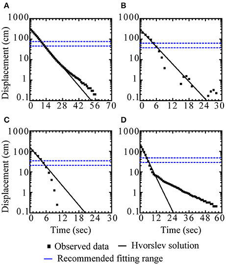
Figure 4. Slug test curve fitting. Water level responses over time (squares), Hvorslev solution (lines) for representative slug tests, and recommended fitting range (blue dashed lines). Water levels generally match the predicted recovery (A), recover rapidly, and sometimes oscillate slightly (B), recover more quickly than predicted (C), or recover more slowly than predicted (D).

Initial water level displacements within the piezometer ranged from 0.3 to 6 m. Despite initial displacements up to 6 m for some slug tests, the Reynolds number is still within the laminar flow range. For this analysis, we assumed that K_z/K_r was 1. A sensitivity analysis showed that decreasing ratio of K_z/K_r from 1 to 0.01 changed the hydraulic conductivity of one slug test from 1.6 × 10⁻⁴ to 2.7 × 10⁻⁴ m/s, which is within the range of variation observed between repeat tests.

Hydraulic conductivity within the firn aquifer was estimated from slug tests using two analysis methods (Supplementary Table 1). Hydraulic conductivity estimated using the Hvorslev method ranges from 1.1 × 10⁻³ to 2.5 × 10⁻⁵ m/s, with a geometric mean of 2.8 × 10⁻⁴ m/s and geometric standard deviation of 1.6. Hydraulic conductivity estimated using the Bouwer and Rice method ranges from 8.8 × 10⁻⁴ to 2.4 × 10⁻⁵ m/s, with a geometric mean of 2.5 × 10⁻⁴ m/s and geometric standard deviation of 1.7 (Table 3). The geometric mean is reported because hydraulic conductivity tends to be log normally distributed (Neuman, 1982). The Hvorselv method yields a larger range in hydraulic conductivity estimates (1.1 × 10⁻³ m/s) than the Bouwer and Rice method (8.5 × 10⁻⁴ m/s). The effective radius over which the water level change occurred ranges from 0.16 m for a test at 12 m depth to 1.18 m for a test at 38 m.

TABLE 3

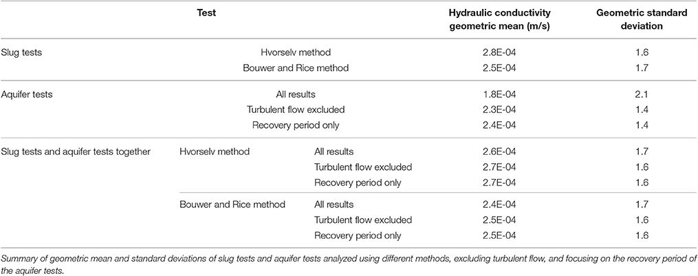
Table 3. Hydraulic conductivity results.

Hydraulic conductivity varies slightly between sites. The hydraulic conductivity decreases slightly with depth through the firn aquifer, although the relationship is weak (r² = 0.17; Figure 5). The greatest decrease with depth occurs at FA16_4. Ice layer stratigraphy does not seem to dramatically influence hydraulic conductivity within the aquifer. This is likely because the horizontal flow induced by the slug test is controlled by the firn with the highest hydraulic conductivity within the screened interval of the piezometer. Further, ice layers can be permeable (Keegan et al., 2014). Humphrey et al. (2012) describe meltwater bypassing ice layers in the percolation zone, a more similar setting to our work than Keegan et al. (2014). Still the general decrease in hydraulic conductivity can be attributed to a gradual increase in density with depth, indicating an increase in ice, which may be more uniformly distributed as opposed to distributed in layers. This is addressed in further detail in Section Discussion.

FIGURE 5

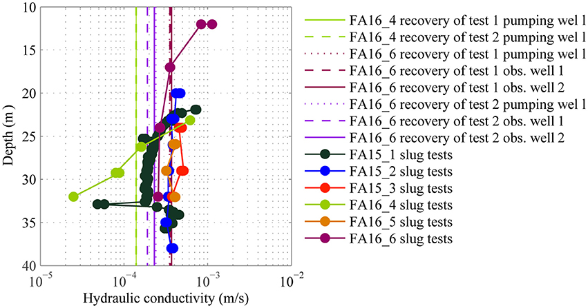
Figure 5. Hydraulic conductivity across ~10 km and between 10–40 m depth. Hydraulic conductivity estimates determined using the Hvorselv method for slug test data and the Theis method for aquifer test data. The slug test measurements were taken at specific depths while the aquifer test data are not depth-specific. Water level rise due to recharge during the aquifer tests has been removed, as has data from the pumping well at site FA16_4 (see Section Aquifer Tests). Data points are larger than standard error of estimate.

The Hvorslev method and Bouwer and Rice methods for estimating hydraulic conductivity yield similar results (Figure 6). The linear fit between the estimates from both methods (y = 0.84 × + 2 × 10⁻⁵ m/s) indicates that the Bouwer and Rice method predicts hydraulic conductivity estimates that are roughly 20% lower than the Hvorslev method. This is consistent with the findings described in Butler (1996) of Hyder et al. (1994) and Hyder and Butler (1995) in terrestrial groundwater systems. The average percent difference between estimates is 8%. The Bouwer and Rice method has been found to underestimate hydraulic conductivity, and yield superior estimates relative to the Hvorslev method (Brown et al., 1995). The largest uncertainty in the hydraulic conductivity estimates from slug tests is that both the Hvorselv and Bouwer and Rice methods ignore the storage properties (specific storage) of the aquifer, which can contribute to uncertainties of over 60% (Brown et al., 1995). However, the difference between the estimates from both methods in this study is ~20%, smaller than the uncertainty from ignoring storage. The mean hydraulic conductivity estimated using both methods are not statistically different, as indicated by a t-test (at p = 0.05). The similarity to each other and to the aquifer test results, described below, indicates that both methods seem to represent the firn aquifer well.

FIGURE 6

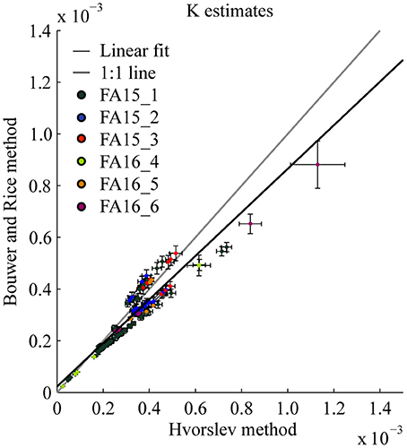
Figure 6. Comparison of hydraulic conductivity estimated using Hvorslev's method and Bouwer and Rice's method for each site. Error bars represent standard error of the hydraulic conductivity estimates. A linear fit of these estimates (black line) has a slope of 0.84, intercept of 2 × 10⁻⁵, and an r² of 0.89 (r = 0.94). The gray line indicates a 1:1 fit.

Aquifer Tests

Aquifer test drawdown and recovery over time, and predicted displacements for a range of hydraulic conductivities are show in Figure 7. The comparisons between observed drawdown and recovery data to theoretical curves predicted by the Theis solution are shown in Figure 8. The hydraulic conductivity estimated from all aquifer tests ranges from 3.7 × 10⁻⁴ to 2.8 × 10⁻⁵ m/s, with a geometric mean of 1.8 × 10⁻⁴ m/s and geometric standard deviation of 1.6 (Tables 3, 4). Changing the ratio of K_z/K_r does not affect hydraulic conductivity estimates. The observed drawdown is close to the predicted drawdown for a hypothetical aquifer test in a 15 m thick aquifer with hydraulic conductivity of 2 × 10⁻⁴ m/s, a pumping rate of 0.001 m³/s and a radial distance of 1 m between the pumping and observation well (Figure 7). Increasing or decreasing the hydraulic conductivity by an order of magnitude results in much larger or smaller displacements than what we observed.

FIGURE 7

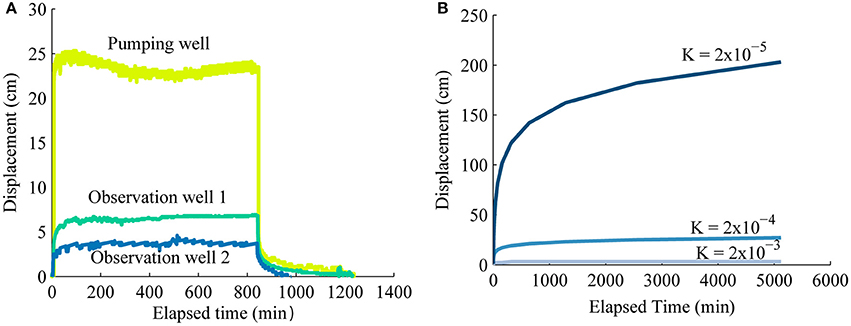
Figure 7. Observed and theoretical drawdown. Displacement over time at site FA16_6 in the pumping and observation wells during the first test (A) and predicted drawdown in an observation well for a hypothetical aquifer test with varying hydraulic conductivity (B). For this scenario, the aquifer is 15 m thick, the pumping rate is 0.0011 m³/s, the storativity is 0.2, and the distance between the pumping and observation well is 1 m. The predicted drawdown when hydraulic conductivity is 2 × 10⁻⁴ m/s is most similar to the drawdown we observed.

FIGURE 8

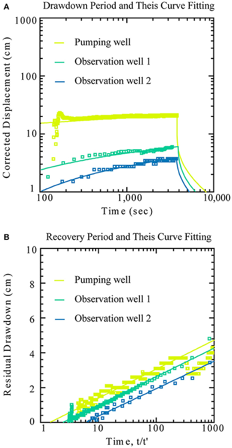
Figure 8. Aquifer test curve fitting. (A) Recharge-corrected drawdown over time and Theis solution curves in the pumping and two observation wells during the second aquifer test at FA16_6. The squares represent water level displacement from the water level prior to pumping in different wells. The lines represent the Theis solution to the drawdown data. (B) Residual drawdown vs. time elapsed since the start of pumping relative to the time since pumping stopped (t/t′) and the Theis solution curves for aquifer test 1 at FA16_6 and FA16_6 The squares represent water level measurements after pumping stops and the lines represent the Theis solution to the recovery data.

TABLE 4

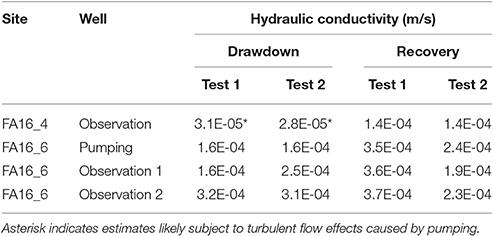
Table 4. Hydraulic conductivity estimates from aquifer tests during drawdown and recovery periods in each well.

The fit between observed and theoretical drawdown for some tests varies. A generally poor fit to early time data probably results from wellbore storage of water and transience in the pumping rate at very early times. The pump gradually increases the pumping rate over the first minute, which violates the constant pumping rate assumption. Wellbore storage serves as the primary source of pumped water at early times, but as pumping continues, wellbore storage decreases and the aquifer becomes the primary source of pumped water. Therefore, many of the early time data (~min) were discarded.

The pumping well at site FA16_4 experienced drawdown below the pressure transducer, causing a loss of data. These data were excluded from hydraulic conductivity estimates. Further, the observation well at site FA16_4 is located only 1 m from the pumping well, and may have been subject to turbulent flow effects caused by pumping as observed in the significantly greater drawdown at this site compared to FA16_6 and the difference between the hydraulic conductivity estimates during the drawdown and recovery periods. Increased and turbulent flow causes head loss in the borehole (Jacob, 1947), which would lead to an underestimation of hydraulic conductivity during the drawdown period. Excluding data influenced by turbulent flow (excluding data from FA16_4 pumping well, and observation well during the drawdown period) results in a range of hydraulic conductivity between 3.7 × 10⁻⁴ and 1.4 × 10⁻⁴ m/s, with a geometric mean of 2.3 × 10⁻⁴ m/s and geometric standard deviation of 1.4.

The displacement data from the recovery period were not influenced by turbulent effects as the pump is not used during this period. Therefore, the recovery data likely result in a more accurate estimate with a range between 3.7 × 10⁻⁴ and 1.4 × 10⁻⁴ m/s, with a geometric mean of 2.4 × 10⁻⁴ m/s and geometric standard deviation of 1.4.

The distance between the pumping and observation wells was measured at the surface, and if the boreholes deviated from vertical, then the true distance between the boreholes may vary. A sensitivity analysis comparing the hydraulic conductivity estimated from the observation well at site FA16_4 showed that increasing the distance between the wells from 1 to 20 m had no effect on the hydraulic conductivity estimate. This is likely because in a highly permeable system, the cone of depression is wide and shallow, and therefore insensitive to the distance between the wells.

The geometric mean of hydraulic conductivity estimated using both slug tests (Hvorselv method) and aquifer tests (only recovery period) is 2.7 × 10⁻⁴ m/s with a geometric standard deviation of 1.4. The hydraulic conductivity decreases most with depth at site FA16_4, shown in the slug test results. The aquifer test at this site indicates that the hydraulic conductivity at this site is roughly the average of the depth-specific slug test measurements.

Discussion

To our knowledge, these are the first hydraulic conductivity measurements of a firn aquifer in the southeastern Greenland ice sheet and these are the first depth specific slug tests conducted in a firn aquifer. We find relatively homogeneous hydraulic conductivity between measurement sites, and a slight decrease with depth. While ice layers within the firn aquifer may reduce vertical hydraulic conductivity, we did not test for this. Ice layers within the aquifer do not appear to dramatically reduce horizontal hydraulic conductivity and thus horizontal flow. Any horizontal fluid flow within the aquifer and discharge into the englacial hydrologic system is controlled by the horizontal firn layers with the highest hydraulic conductivity. Quantifying hydraulic conductivity and its spatial variation is a crucial step in developing realistic hydrologic models of the aquifer systems, and for understanding the impact the firn aquifer has on ice sheet mass balance. The observed spatial and vertical homogeneity should reduce firn aquifer hydraulic modeling complexity.

The largest uncertainties in the hydraulic conductivity estimates from slug tests result from ignoring the storage properties of the aquifer, and possible leakage around the packer. This could contribute to the weak vertical gradient in hydraulic conductivity. However, water level differences were observed as the packer was inflated, suggesting that the seal was strong enough to counter the hydraulic gradient. The largest uncertainties in the hydraulic conductivity estimates from the aquifer tests likely result from turbulent effects in this highly permeable system. The high permeability of the aquifer meant that the observation wells had to be placed close to the pumping well in order to observe any measurable drawdown. However, this also resulted in some turbulent effects in the water level data (much lower hydraulic head than predicted), leading to a poor fit to theoretical solutions, particularly in the pumping well. This was addressed by discarding data where these effects were obvious, and by fitting the theoretical curves to the later time data and the recovery period data.

Although, the very early time recovery data (~seconds) may be subject to turbulent effects, most of it is not. The recovery data, particularly in the observation wells, are also not subject to influences by well construction. These data depend solely on aquifer parameters. The recovery data are also not subject to any turbulent effects from pumping and are therefore the more reliable data and provide the most reliable estimate of hydraulic conductivity. Further, the general agreement with the hydraulic conductivity estimates from multiple sites and methods suggests that the hydraulic conductivity of the system is generally well-represented. The agreement between the slug tests and the aquifer tests, which perturb a larger volume of the aquifer (over 10 m diameter), suggests that meltwater from the installation of the piezometer or drilling of the borehole does not seem to impact the hydraulic conductivity estimates. Numerical modeling combined with an independent measurement of fluid flow, can better constrain hydraulic conductivity. In the absence of an independent measurement of flow, the in situ measurements described in this manuscript represent the best estimates of hydraulic conductivity. The overall range of hydraulic conductivity values seems to capture the uncertainty.

The porosity and permeability of the firn could be altered by the melting caused by the heated piezometer or the heated thermoelectric drill. This would particularly bias the slug test results toward a higher hydraulic conductivity because they perturb a relatively smaller volume of the aquifer. However, the aquifer test results, which perturb a much larger volume of the aquifer (>10 m diameter), are less subject to significant alteration from melting and provide a good comparison to, and generally agree with, the slug test results. The agreement between multiple complementary methods (slug tests and aquifer tests during pumping and recovery periods in particular) suggests that the hydraulic conductivity estimates are robust.

No seasonal changes were observed in hydraulic conductivity. However, only one site was tested in the spring, prior to surface melt onset. The other five sites were tested in the summer. Still, we do not expect substantial changes to hydraulic conductivity within the saturated zone because the temperature within the saturated zone remains at 0°C throughout the year. Thus, we do not expect significant freezing or thawing to occur within the saturated zone, which could alter the hydraulic conductivity by reducing or enhancing pore connectivity. However, longer time monitoring in different seasons would be required to identify seasonal impacts.

Our measurements of the hydraulic conductivity of the firn aquifer in southeast Greenland overlap with estimates for a firn aquifer in the Holtedahlfonna ice field, Svalbard, between 3.2 × 10⁻⁵ and 1.8 × 10⁻⁴ m/s (Christianson et al., 2015). The hydraulic conductivities measured in southeast Greenland, however, are approximately an order of magnitude higher than those taken from firn aquifers in various mountain glaciers where hydraulic conductivities show a relatively narrow range from 1.2 × 10⁻⁵ to 5 × 10⁻⁵ m/s (Oerter and Moser, 1982; Oerter et al., 1983; Fountain, 1989; Fountain and Walder, 1998; Schneider, 1999; Jansson et al., 2003). Hydraulic conductivity depends on the properties of the porous media (e.g., grain size, shape, or packing) and the fluid flowing through the porous media. Christianson et al. (2015) hypothesized that aquifers at deeper locations within an ice sheet/glacier will have decreased conductivities as firn densifies and pore space decreases. While this hypothesis may generally hold for a firn column in a single location, the growing number of spatially distributed hydraulic conductivity measurements of firn show variations across glaciers and ice sheets. This is expected as firn stratigraphy and microstructure vary across climates.

We can also compare permeability, which is only a function of the porous media, to sites where no aquifer exists. Permeability increases from mountain glaciers (~10⁻¹² m²) to the southeast Greenland firn aquifer (~10⁻¹² to 10⁻¹⁰ m²) to dry firn (~10⁻¹⁰ m²) (Oerter and Moser, 1982; Oerter et al., 1983; Fountain, 1989; Fountain and Walder, 1998; Schneider, 1999; Albert et al., 2000; Luciano and Albert, 2002; Adolph and Albert, 2014; Keegan et al., 2014). We attribute the difference in permeability across regions to the ice content represented in density profiles of the different locations where average density decreases from mountain glaciers to southeast Greenland firn aquifer to dry firn (Fountain, 1989; Adolph and Albert, 2014; Koenig et al., 2014). Although, Keegan et al. (2014) and Adolph and Albert (2014), and Albert et al. (2000) report vertical permeability, Keegan et al. (2014) note that differences between lateral and vertical permeability are smaller than differences between vertical permeability of different layers (see Luciano and Albert, 2002), and are therefore adequate for a general comparison. Also, the horizontal and vertical permeability are within the same order of magnitude. The density profiles recorded at measurement sites offer an initial explanation, as follows, for the changes in permeability; however, detailed microstructure measurements are needed, specifically to resolve pore interconnectivity and orientation, to more fully describe permeability differences.

The differences in ice content, and therefore densities, between mountain glaciers and the southeast Greenland firn aquifer are in part due to the long-term (decades), perennial nature of the aquifer in southeast Greenland. Aquifers in mountain glaciers are generally smaller, thinner, and steeper, allowing for annual drainage and more refreeze when air temperatures dip below 0°C in the winter (Vallon et al., 1976; Oerter et al., 1983; Fountain, 1989, 1996; Jansson et al., 2003). The perennial aquifer in southeast Greenland is in general deeper (10's of m) and thicker (10's of m), which limits refreezing in the saturated zone (Table 2). This increased annual refreezing in mountain glaciers likely leads to more ice and reduced pore connectivity.

The differences in ice content between dry firn and the southeast Greenland firn aquifer are due to climatic and geographic differences (Kuipers Munneke et al., 2014). The dry-firn sites experience little to none of the surface melt and subsequent freezing that occurs at our site, in the percolation zone of southeast Greenland. Therefore, the dry-firn sites do not accumulate as much refrozen ice, leading to more permeable firn.

The lateral homogeneity of hydraulic conductivity observed in the Greenland firn aquifer has also been observed in South Cascade Glacier (Fountain, 1989). This similarity likely reflects the homogenizing effect of saturating firn at 0°C on firn microstructure. While the ice layer stratigraphy at a specific location doesn't seem to dramatically influence the horizontal hydraulic conductivity, as shown in our measurements and noted by Keegan et al. (2014), increases in overall ice content of the firn column do seem to reduce hydraulic conductivity and permeability (e.g., from mountain glaciers to water saturated firn to dry firn).

This study provides estimates on hydraulic parameters for a newly discovered firn aquifer and proves the effectiveness of the heated piezometer, particularly as a light weight (~200 kg), fast method to access an aquifer from the snow surface for in situ physical measurements and water sampling. The heated piezometer is a unique tool developed to study firn hydrology in Greenland, but can be used in any firn aquifer setting. The hydraulic conductivities measured can be used to improve models of water flow within, and discharge from, firn aquifers and further constrain the storage and retention time estimates for aquifers within the Greenland ice sheet. As melt is projected to increase under a predicted warmer climate, the firn aquifer could have an increasingly important effect on Greenland ice sheet mass balance by efficiently transporting meltwater through firn to the ocean.

Author Contributions

OM collected field data, conducted analysis and interpretation, and wrote the manuscript. DS designed and built heated piezometer, collected field data, and consulted on data analysis and manuscript writing and editing. CM, LK, RF, LM, NS, SL, AL, and LB assisted with field work, contributed to intellectual content, and contributed to manuscript writing.

Funding

This work was supported by NSF grant number PLR-1417987. LM and NS were supported by PLR-1417993. LK and LB were supported by NASA Cryospheric Sciences program NASA Award NNX15AC62G. SL was supported by an NOW ALW Veni grant, number 865.15.023.

Conflict of Interest Statement

The authors declare that the research was conducted in the absence of any commercial or financial relationships that could be construed as a potential conflict of interest.

The handling Editor declared a shared affiliation, though no other collaboration, with one of the authors LK and states that the process nevertheless met the standards of a fair and objective review.

Acknowledgments

The authors thank Kyli Cosper, Kathy Young, and the entire CH2M Polar Field Services team for logistical assistance. Thanks also to Josh Goetz and IDDO for drilling support in April, 2015 and Jay Kyne for drill consultation and development. We also thank the editor and reviewers for thoughtful comments that greatly improved this manuscript.

Supplementary Material

The Supplementary Material for this article can be found online at: https://www.frontiersin.org/article/10.3389/feart.2017.00038/full#supplementary-material

Footnotes

1. ^Duffield, G. M. AQTESOLV. HydroSOLVE, Inc. Available online at: http://www.aqtesolv.com/

References

Adolph, A. C., and Albert, M. R. (2014). Gas diffusivity and permeability through the firn column at Summit, Greenland: measurements and comparison to microstructural properties. Cryosphere 8, 319–328. doi: 10.5194/tc-8-319-2014

CrossRef Full Text | Google Scholar

Albert, M. R., and Shultz, E. F. (2002). Snow and firn properties and air–snow transport processes at Summit, Greenland. Atmos. Environ. 36, 2789–2797. doi: 10.1016/S1352-2310(02)00119-X

CrossRef Full Text | Google Scholar

Albert, M. R., Shultz, E. F., and Perron, F. E. (2000). Snow and firn permeability at Siple Dome, Antarctica. Ann. Glaciol. 31, 353–356. doi: 10.3189/172756400781820273

CrossRef Full Text | Google Scholar

Albert, M., Shuman, C., Courville, Z., Bauer, R., Fahnestock, M., and Scambos, T. (2004). Extreme firn metamorphism: impact of decades of vapor transport on near-surface firn at a low-accumulation glazed site on the East Antarctic plateau. Ann. Glaciol. 39, 73–78. doi: 10.3189/172756404781814041

CrossRef Full Text | Google Scholar

Alley, R. B., Dupont, T. K., Parizek, B. R., and Anandakrishnan, S. (2005). Access of surface meltwater to beds of sub-freezing glaciers: preliminary insights. Ann. Glaciol. 40, 8–14. doi: 10.3189/172756405781813483

CrossRef Full Text | Google Scholar

Bouwer, H. (1989). The bouwer and rice slug test - an update. Groundwater 27, 304–309. doi: 10.1111/j.1745-6584.1989.tb00453.x

CrossRef Full Text | Google Scholar

Bouwer, H., and Rice, R. C. (1976). A slug test for determining hydraulic conductivity of unconfined aquifers with completely or partially penetrating wells. Water Resour. Res. 12, 423–428. doi: 10.1029/WR012i003p00423

PubMed Abstract | CrossRef Full Text | Google Scholar

Bredehoeft, J. D., Cooper, H. H., and Papadopulos, I. S. (1966). Inertial and storage effects in well-aquifer systems: an analog investigation. Water Resour. Res. 2, 697–707. doi: 10.1029/WR002i004p00697

CrossRef Full Text | Google Scholar

Brown, D. L., Narasimhan, T. N., and Demir, Z. (1995). An evaluation of the Bouwer and Rice method of slug test analysis. Water Resour. Res. 31, 1239–1246. doi: 10.1029/94WR03292

CrossRef Full Text | Google Scholar

Butler, J. J. J. (1996). Slug tests in tite characterization: some practical considerations. Environ. Geosci. 3, 154–163.

Google Scholar

Butler, J. J. J. (1997). The Design, Performance, and Analysis of Slug Tests. New York, NY: CRC Press.

Google Scholar

Christianson, K., Kohler, J., Alley, R. B., Nuth, C., and van Pelt, W. J. J. (2015). Dynamic perennial firn aquifer on an Arctic glacier. Geophys. Res. Lett. 42, 1418–1426. doi: 10.1002/2014GL062806

CrossRef Full Text | Google Scholar

Chu, V. W. (2014). Greenland ice sheet hydrology: a review. Prog. Phys. Geogr. 38, 19–54. doi: 10.1177/0309133313507075

CrossRef Full Text | Google Scholar

Das, S. B., Joughin, I., Behn, M. D., Howat, I. M., King, M. A., Lizarralde, D., et al. (2008). Fracture propagation to the base of the Greenland ice sheet during Supraglacial Lake drainage. Science 320, 778–781. doi: 10.1126/science.1153360

PubMed Abstract | CrossRef Full Text | Google Scholar

Ferris, J. G., Knowles, D. B., Brown, R. H., and Stallman, R. W. (1962). Theory of Aquifer Tests. Water Supply Paper U.S. Geological Survey, 174.

Forster, R. R., Box, J. E., van den Broeke, M. R., Miège, C., Burgess, E. W., van Angelen, J. H., et al. (2014). Extensive liquid meltwater storage in firn within the Greenland ice sheet. Nat. Geosci. 7, 1–4. doi: 10.1038/ngeo2043

CrossRef Full Text

Fountain, A. G. (1989). The storage of water in, and hydraulic characteristics of, the firn of South Cascade Glacier, Washington State, USA. Ann. Glaciol. 13, 69–75.

Google Scholar

Fountain, A. G. (1996). Effect of snow and firn hydrology on the physical and chemical characteristics of glacial runoff. Hydrol. Process. 10, 509–521. doi: 10.1002/(SICI)1099-1085(199604)10:4<509::AID-HYP389>3.0.CO;2-3

CrossRef Full Text | Google Scholar

Fountain, A. G., and Walder, J. S. (1998). Water flow through temperate glaciers. Rev. Geophys. 36:299. doi: 10.1029/97RG03579

CrossRef Full Text | Google Scholar

Freeze, A., and Cherry, J. (1979). Groundwater. Englewood Cliffs, NJ: Prentice Hall.

Garber, M. S., and Koopman, F. C. (1968). Methods of Measuring Water Levels in Deep Wells. U.S. Geological Survey Techniques of Water-Resources Investigations, 23.

Harper, J., Humphrey, N., Pfeffer, W. T., Brown, J., and Fettweis, X. (2012). Greenland ice-sheet contribution to sea-level rise buffered by meltwater storage in firn. Nature 491, 240–243. doi: 10.1038/nature11566

PubMed Abstract | CrossRef Full Text | Google Scholar

Helm, V., Humbert, A., and Miller, H. (2014). Elevation and elevation change of Greenland and Antarctica derived from CryoSat-2. Cryosphere 8, 1539–1559. doi: 10.5194/tc-8-1539-2014

CrossRef Full Text | Google Scholar

Humphrey, N. F., Harper, J. T., and Pfeffer, W. T. (2012). Thermal tracking of meltwater retention in Greenland's accumulation area. J. Geophys. Res. 117, F01010. doi: 10.1029/2011JF002083

CrossRef Full Text | Google Scholar

Hvorslev, M. J. (1951). Time Lag and Soil Permeability in Ground-Water Observations. Bull. no. 36 (Vicksburg, MS: Waterways Experiment Station, U.S. Army Corps of Engineers), 53.

Google Scholar

Hyder, Z., and Butler, J. J. J. (1995). Slug tests in unconfined formations: an assessment of the Bouwer and Rice technique. Ground Water 33, 16–22. doi: 10.1111/j.1745-6584.1995.tb00258.x

CrossRef Full Text | Google Scholar

Hyder, Z., Butler, J. J. J., McElwee, C. D., and Liu, W. (1994). Slug tests in partially penetrating wells. Water Resour. Res. 30, 2945–2957. doi: 10.1029/94WR01670

CrossRef Full Text | Google Scholar

Iken, A., Fabri, K., and Funk, M. (1996). Water storage and subglacial drainage conditions inferred from borehole measurements on Gornergletscher, Valais, Switzerland. J. Glaciol. 42, 233–248.

Google Scholar

Jacob, C. E. (1944). Notes on Determining Permeability by Pumping Tests under Watertable Conditions. US Geological Survey Open File Report.

Jacob, C. E. (1947). Drawdown test to determine effective radius of artesian well. Trans. Am. Soc. Civ. Eng. 112, 1047–1064.

Google Scholar

Jansson, P., Hock, R., and Schneider, T. (2003). The concept of glacier storage: a review. J. Hydrol. 282, 116–129. doi: 10.1016/S0022-1694(03)00258-0

CrossRef Full Text | Google Scholar

Joughin, I., Das, S. B., King, M. A., Smith, B. E., Howat, I. M., and Moon, T. (2008). Seasonal speedup along the Western flank of the Greenland ice sheet. Science 320, 781–783. doi: 10.1126/science.1153288

PubMed Abstract | CrossRef Full Text | Google Scholar

Keegan, K., Albert, M. R., and Baker, I. (2014). The impact of ice layers on gas transport through firn at the North Greenland Eemian Ice Drilling (NEEM) site, Greenland. Cryosphere 8, 1801–1806. doi: 10.5194/tc-8-1801-2014

CrossRef Full Text | Google Scholar

Koenig, L. S., Miege, C., Forster, R. R., and Brucker, L. (2014). Initial in situ measurements of perennial meltwater storage in the Greenland firn aquifer. Geophys. Res. Lett. 41, 81–85. doi: 10.1002/2013GL058083

CrossRef Full Text | Google Scholar

Kruseman, G. P., De Ridder, N. A., and Verwei, J. M. (1994). Analysis and Evaluation of Pumping Test Data, 2nd Edn. Wageningen: ILRI Publication.

Kuipers Munneke, P., Ligtenberg, S. R. M., van den Broeke, M. R., van Angelen, J. H., and Forster, R. R. (2014). Explaining the presence of perennial liquid water bodies in the firn of the Greenland Ice Sheet. Geophys. Res. Lett. 41, 476–483. doi: 10.1002/2013GL058389

CrossRef Full Text | Google Scholar

Kulessa, B., Hubbard, B., Williamson, M., and Brown, G. H. (2005). Hydrogeological analysis of slug tests in glacier boreholes. J. Glaciol. 51, 269–280. doi: 10.3189/172756505781829458

CrossRef Full Text | Google Scholar

Lewis, S. M., and Smith, L. C. (2009). Hydrologic drainage of the Greenland Ice Sheet. Hydrol. Process. 23, 2004–2011. doi: 10.1002/hyp.7343

CrossRef Full Text | Google Scholar

Luciano, G. L., and Albert, M. R. (2002). Bidirectional permeability measurements of polar firn. Ann. Glaciol. 35, 63–66. doi: 10.3189/172756402781817095

CrossRef Full Text | Google Scholar

Machguth, H., MacFerrin, M., van As, D., Box, J. E., Charalampidis, C., Colgan, W., et al. (2016). Greenland meltwater storage in firn limited by near-surface ice formation. Nat. Clim. Chang. 6, 390–393. doi: 10.1038/nclimate2899

CrossRef Full Text | Google Scholar

Meierbachtol, T. W., Harper, J. T., Humphrey, N. F., Shaha, J., and Bradford, J. H. (2008). Air compression as a mechanism for the underdamped slug test response in fractured glacier ice. J. Geophys. Res. 113:F04009. doi: 10.1029/2007JF000908

CrossRef Full Text | Google Scholar

Miège, C., Forster, R. R., Brucker, L., Koenig, L. S., Solomon, D. K., Paden, J. D., et al. (2016). Spatial extent and temporal variability of Greenland firn aquifers detected by ground and airborne radars. J. Geophys. Res. Earth Surf. 121, 2381–2398. doi: 10.1002/2016JF003869

CrossRef Full Text | Google Scholar

Neuman, S. P. (1982). Statistical characterization of aquifer heterogeneities: an overview. GSA Spec. Pap. 189, 81–102. doi: 10.1130/SPE189-p81

CrossRef Full Text | Google Scholar

Oerter, H., and Moser, H. (1982). “Water storage and drainage within the firn of a temperate glacier (Vernagtferner, Oetztal Alps, Austria),” in Hydrological Aspects of Alpine and High Mountain Areas, ed J. W. Glen (Exeter: Proceedings Exeter Symposium), 71–81.

Google Scholar

Oerter, H., Reinwarth, O., and Rufli, H. (1983). Core drilling through a temperate alpine glacier (Vernagtferner, Oetztal Alps) in 1979. Z. Gletscherkd. Glazialgeol. 18, 1–11.

Google Scholar

Pfeffer, W. T., Meier, M. F., and Illangasekare, T. H. (1991). Retention of Greenland runoff by refreezing: implications for projected future sea level change. J. Geophys. Res. 96:22117. doi: 10.1029/91JC02502

CrossRef Full Text | Google Scholar

Poinar, K., Joughin, I., Lilien, D., Brucker, L., Kehrl, L., and Nowicki, S. (2017). Drainage of Southeast Greenland firn aquifer water through crevasses to the bed. Front. Earth Sci. 5:5. doi: 10.3389/FEART.2017.00005

CrossRef Full Text | Google Scholar

Schneider, T. (1999). Water movement in the firn of Storglaciaren, Sweden. J. Glaciol. 45, 286–294. doi: 10.3189/002214399793377211

CrossRef Full Text | Google Scholar

Smith, L. C., Chu, V. W., Yang, K., Gleason, C. J., Pitcher, L. H., Rennermalm, A. K., et al. (2015). Efficient meltwater drainage through supraglacial streams and rivers on the southwest Greenland ice sheet. Proc. Natl. Acad. Sci. U.S.A. 112, 1001–1006. doi: 10.1073/pnas.1413024112

PubMed Abstract | CrossRef Full Text | Google Scholar

Sole, A. J., Mair, F. D. W., Nienow, P. W., Bartholomew, I. D., King, M. A., Burke, M. J., et al. (2011). Seasonal speedup of a Greenland marine-terminating outlet glacier forced by surface melt–induced changes in subglacial hydrology. J. Geophys. Res. 116:F03014. doi: 10.1029/2010JF001948

CrossRef Full Text | Google Scholar

Stone, D. B., and Clark, G. C. (1972). Estimation of subglacial hydraulic properties frotn induced changes in basal water pressure: a theoretical fratnework for borehole-response tests. J. Glaciol. 39, 327–340.

Theis, C. V. (1935). The relation between the lowering of the piezometric surface and the rate and duration of discharge of a well using ground-water storage. Trans. Am. Geophys. Union 16, 519–524. doi: 10.1029/TR016i002p00519

CrossRef Full Text | Google Scholar

Tóth, J. (1963). A theoretical analysis of groundwater flow in small drainage basins. J. Geophys. Res. 68, 4795–4812. doi: 10.1029/JZ068i016p04795

CrossRef Full Text | Google Scholar

Vallon, M., Petit, J.-R., and Fabre, B. (1976). Study of an ice core to the bedrock in the accumulation zone of an Alpine glacier. J. Glaciol. 17, 13–28.

Google Scholar

Van der Kamp, G. (1976). Determining aquifer transmissivity by means of well response tests: the underdamped case. Water Resour. Res. 12, 71–77. doi: 10.1029/WR012i001p00071

CrossRef Full Text | Google Scholar

Zwally, H. J. (2002). Surface melt-induced acceleration of greenland ice-sheet flow. Science 297, 218–222. doi: 10.1126/science.1072708

PubMed Abstract | CrossRef Full Text | Google Scholar