Weekly Glacier Flow Estimation from Dense Satellite Time Series Using Adapted Optical Flow Technology

1. Introduction

In recent years, the focus in optical remote sensing has shifted from the use of a few scenes from individual satellites toward exploitation of full constellations. Twin satellites or flocks of satellites have been launched, sensing the globe with ever shorter revisit times. The advantages of short temporal sampling rates for glaciology are now being investigated (Fahnestock et al., 2015). One of these opportunities has been the exploration of short term changes in glacier flow, on the scale of an individual season (Berthier et al., 2005; Armstrong et al., 2016). These demonstrations focus on specific glaciers through targeted acquisitions. However, newly launched earth observation constellations are designed to sense almost continuously in a non-discriminate fashion. This process is facilitated through commercial constellations of satellites, as some sense the globe daily with high resolution (Planet Team, 2017). Continuous sensing is also facilitated through multiple public constellations (e.g., Landsat 8 and Sentinels-2A and -2B) when combined, reduce revisit times from weekly to daily timescales, particularly toward the poles. With the technique proposed here, it may be possible to detect local, short-lived events, such as speed-up events, glacier outbursts (jökulhlaup), calving, surging, or galloping on any glacier.

The advancement of satellite technology has pushed the typical bottleneck of (glacier) remote sensing from data availability to the exploration and processing of large data volumes. Glacier displacement estimation from optical remote sensing has traditionally been done by matching patterns from two subsequent image subsets. The displacement is rooted from a voting over candidate displacements where the similarity is maximized, or its difference in appearance minimized. This pair-based processing is computationally intensive and inefficient, because of its two-dimensional search space, and its simple “winner takes all” approach. This could partially be overcome by including a third image (Altena and Kääb, 2017), but that approach would only enhance the reliability not the processing load. Furthermore, because of the vast amount of imagery within the archives, selection of the best pair might be troublesome, as cloud cover hampers the visibility and adequate cloud detection methods are not yet available for every constellation. Bulk processing of the Landsat 8 archive has recently become operational (Scambos et al., 2016). The vast collection of velocity fields has a wealth of information within, and makes it possible to assess glacier velocity on regional or global scale. Yet this still has not solved the data volume problem, as the velocity data needs to be converted into information or filtered through advanced post-processing procedures, which have not operated at an adequate level. Consequently, alternative approaches have come into sight. One possible strategy includes the implementation of exploratory and quantitative tools, which enable the rapid and reliable extraction of information from remote sensing data. This is the aim of our study; the ability to identify the temporal flow behavior of a glacier within a large collection of remote sensing images without having to match a large number of image pair combinations.

A second concern is the concept behind standard image matching. Standard image matching is a useful tool for measuring larger displacements, but is not optimal for small displacements or noisy time-series. The common framework of image matching finds the displacement of two sub-windows from orthorectified images (Scambos et al., 1992; Kääb and Vollmer, 2000; Heid and Kääb, 2012). Typically, the estimated precision of image matching ranges between 1/2 (Prasad et al., 1992) down to 1/16 (Debella-Gilo and Kääb, 2011) of a pixel. Several requirements must be met in order to establish a successful match. First, the displacement must be statistically significant in order to be observable. However, before any sufficient displacement has occurred on a glacier, the appearance of observable surface features might have degraded. Appearance of an image can change over time (due to snow cover changes and ice melt, for instance) or space (surface deformation instead of simple translation). These surface processes greatly modify the configuration of the surface pattern, and thus the matching quality. Because of these requirements, which can contradict each other, most studies focus on large valley glaciers, or converging glacial outlets which have considerable speed. However, the majority of glaciers move slow and extracted displacements with optical satellite-based remote sensing from these are still a challenge, which we aim to tackle here.

The glaciological community lacks sufficient processing approaches for large volume data exploration. It is therefore useful to investigate how other scientific fields handle the processing of displacements from dense image time-series. Ideally, glaciologists need a method which is robust, sensor independent, and able to process vast amounts of data. Here, we introduce one such methodology, based on a combination of optical flow technology (from computer vision) and particle tracking velocimetry (which is an established technique in experimental fluid mechanics). The advantage of such an approach is its simplicity in formulation and implementation. The achievable localization occurs at the resolution of an individual pixel. The applicability of this methodology is highlighted on a continental mountain glacier in Yukon, Canada, and a maritime glacier on Svalbard: Kronebreen. We first introduce the data, then provide background for our hybrid methodology. We then describe our actual implementation, present and discuss our case study results, and finally draw perspectives and conclusions.

2. Background

Acquiring images with a high repetition-rate with respect to the movement rate of the object is a new possibility in remote sensing and glaciology. However, such a setup is common practice in computer vision and experimental fluid mechanics where imaging is often done under controlled laboratory conditions with almost free choice of acquisition frequency. Both latter fields of science have thus well-developed methods to extract displacement fields under such conditions, not least optical flow and particle tracking velocimetry.

2.1. Strategies of Glacier Flow Estimation

Prior to our discussion of technical content, we wish to clarify our nomenclature, as a wide range of names exist for image-matching. Names are mostly a combination of a starting term such as, speckle, offset, feature, pattern, chip, and image, followed by, matching, sampling, or tracking.

In image matching, a subset of an image is taken and searched for in the second image. A brute force or ad-hoc strategy is applied and image subsets on a regular grid with overlap are processed. Commonly the imagery is pre-processed by applying a band-pass filter (Scambos et al., 1992) or a filter-bank (Ahn and Howat, 2011), in order to enhance the pattern within the image. The size of the subset is dependent on the amount of information within the pattern, which is used to establish a unique similarity. The resulting displacement or offset estimate is therefore a group velocity of the contributing pattern within this subset (Debella-Gilo and Kääb, 2012).

Another strategy includes a search for pronounced features (Tuytelaars and Mikolajczyk, 2008) (intensity corners or blobs) and the process of finding these features in other acquisitions. The mating of features is done by finding correspondences through descriptors and solving an assignment problem. The field glaciology has not engaged this technique, but it may be a promising approach because the strategy is efficient and as there is an increase of volume from available remote sensing data. This strategy also changes the mathematical framework of the information extracted. Image matching is mostly operating in an Eulerian framework, while feature (or particle) tracking is a Lagrangian framework. Transforming from one to the other is done through the material derivative,

$\begin{array}{cc}\frac{d\overrightarrow{u}}{dt}=\frac{\partial \overrightarrow{u}}{\partial t}+(\nabla \cdot \overrightarrow{u})\overrightarrow{u}.& \left(1\right)\end{array}$

The difference between both systems is not very distinct when an image pair is used. However, the nomenclature becomes important when more than two instances in time are taken into account. The use of tracking implies to follow a specific feature within the fluid, thus is in a Lagrangian framework. While sampling might imply a site specific sensing strategy with fixed positions, corresponding to a Eulerian framework.

2.2. Optical Flow

There is a rich body of literature on optical flow (Barron et al., 1994; Baker et al., 2011). The field has continued to evolve since its introduction in the 1980's (Horn and Schunck, 1981). The optical flow problem can be formulated as,

$\begin{array}{cc}\frac{\partial I}{\partial t}=\frac{\partial I}{\partial x}\frac{\partial x}{\partial t}+\frac{\partial I}{\partial y}\frac{\partial y}{\partial t}.& \left(2\right)\end{array}$

Here, I denotes the intensity of a pixel within the image, and the derivatives are in space (x, y) and time (t). The right side of the equation is a common entity for many studies in glaciology. The gradient operators are used to enhance edges, and off course the velocity field ($\frac{dx}{dt},\frac{dy}{dt}$) is the component searched for through optical pattern matching. The left-hand-side of the equation is, to our best knowledge, only highlighted in Bindschadler et al. (2010). In that study, visually stable icesheet imagery was differenced, and directly related to changes in the slope of the terrain. A connection to movement was not made, though this was done by Kääb (2005), see their Figures 4–7, but only in a qualitative manner of change/no-change.

The advantage of this formulation is its ability to work at the level of individual pixels, while image matching needs a support region of several pixels. Consequently, derivative products, such as strain rates, can have a higher spatial resolution. But the system of equations in Equation (2) is ill-posed, and can only be solved in a global approach through regularization, where in general a constraint on the curvature of the velocity field is given. Alternatively, a local approach can be taken, where Equation (2) is formulated as linear system of equations. In this approach, the neighborhood is taken into the least squares estimation in order to make the design matrix full-rank. An assessment of optical flow methodologies for glacier flow has been done by Vogel et al. (2012), however the results were not encouraging. One reason might have been the temporal baseline of the images, which were taken a year apart, and which resulted in considerable change of surface features.

In order for optical flow to work reliably, the constraint of consistency of brightness should hold, because illumination changes (left-hand-side of Equation 2) always resolve in movement (right-hand-side). However, two effects interfere with this constraint. First, glaciers are partially covered by snow, which has a certain reflection curve. As snow “ages,” the grain size increases and the reflection intensity decreases (Warren, 1982). Second, a considerable portion of glaciers is situated at high latitudes. Consequently, irradiance varies as the sun elevation changes rapidly in autumn and spring. These two processes are highly influential, such that finding acquisitions which do satisfy the brightness consistency constraint is difficult. Hence, direct use of typical past and current satellite image time series for optical flow is not useful in general.

2.3. Particle Tracking Velocimetry

In experimental fluid mechanics, the flow of fluids is examined through recording a fluid seeded with particles or grains using high frame-rate cameras. Again, the literature is very rich (Maas et al., 1993; Guezennec et al., 1994) and references given here are therefore limited. Within particle tracking velocimetry also cross-breeding is found where optical flow is solved within a stream function (Heitz et al., 2010; Luttman et al., 2013). When the rate of displacement is more than several pixels, the main methods used are based on matching windows according to similarity. This pattern matching technique is known as Particle Image Velocimetry (PIV) (Sveen and Cowen, 2004; Raffel et al., 2013). These experiments are done in a laboratory setting, where influencing parameters are highly controlled. For in-plain flow the particles are lighted with a lightsheet and the camera is aligned perpendicular to this plain. The resulting imagery is transformed to a binary image by a threshold and converted to features. Features in consecutive images are then connected through a nearest neighbor search. This is robust, because the movement is within the pixel. When longer displacements occur or the seeding of particles increases this methodology needs regularization and transforms into a correspondence problem.

Again, if this methodology is directly related to glacier flow some complications appear. First, the observed features on a glacier are dynamic in appearance. On a glacier, features have different time scales, and may exist for decades (ogive), years (looped morain), months (crevasse), weeks (meltwater channel), or days (snow patch). Snow cover can cause features to appear and reappear, which forces the thresholding to be adaptive. Furthermore, it is difficult to specify what a traceable feature is, as the feature can be a dust pattern of several meters or a slim melting channel, for instance. But particle tracking velocimetry has methodological elements that are potentially useful for glacier movement estimation.

2.4. Space-Time

A third view-angle tries to look at repeat images through the transformation to space-time imaging. If displacement is reduced to motion (dx/dt) in a known direction, a scatterer has a certain position (X) and reflected intensity,

$\begin{array}{cc}{X}_{t=i+1}=\frac{dx}{dt}\cdot t+X_{t=i}.& \left(3\right)\end{array}$

This is a first-order Taylor extension and grasps the concept that velocity is orientation in the space-time domain (Adelson and Bergen, 1985; Bruce et al., 2003). A conceptual drawing might illustrate this concept better, as is done in Figure 1. Thus, if repeat images are stacked, forming a cube of voxels, any slice through the cube in the third dimension (vertical dimension in Figure 1) will give a space-time image (i.e., horizontal axes: space; vertical axis: time). When the sampling is regular over time, it is possible to estimate speed directly within such space-time image through the use of directional filters (Freeman and Adelson, 1991). When transforming the space-axis to the direction of motion, Equation (2) is much simplified, and velocity can directly be estimated:

$\begin{array}{cc}\frac{\partial I}{\partial t}/\frac{\partial I}{\partial x}=\frac{\partial x}{\partial t}.& \left(4\right)\end{array}$

These relationships have been exploited within the computer vision community, recently it has evolved into a branch known as video magnification (Wadhwa et al., 2013). Even when outdoor scenes are used in video magnification, the sampling interval is sufficiently high, so that the data complies with the above brightness consistency constraint. Similar advances have been implemented in the field of ocean sciences, see for an extensive account (Jähne, 1993). Again the data have mostly been collected in laboratory settings or had strong coherence in appearance. More complicated flow has been analyzed such as blood flow (Chen et al., 2011), but again this is done in a situation where illumination and features are stable. These approaches might be of particular use for repeat Synthetic Aperture Radar (SAR) imagery, as glacial features are more visually coherent in this type of data over short time scales due to active illumination.

FIGURE 1

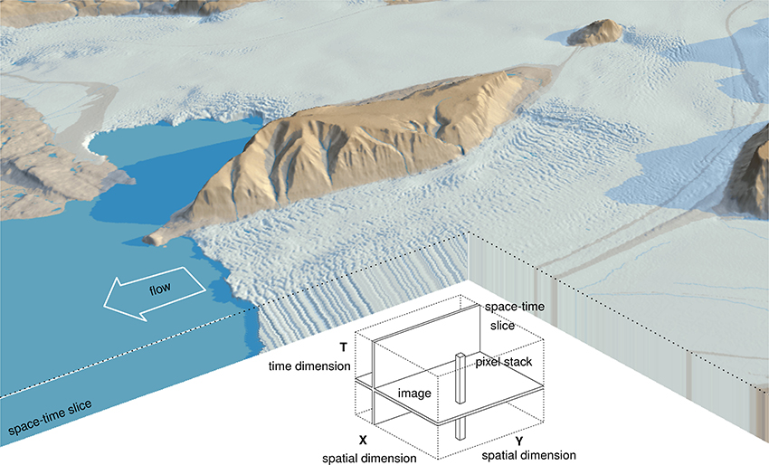
Figure 1. Schematic illustration of an image stack. In the background is the interpretation of such a slice. Movement in the spatial domain results in orientation in the space-time domain. The 3D background image shows Kronebreen, image courtesy of mapping division at Norwegian Polar Institute.

3. Data and Sites

Landsat 8 acquires imagery every 16 days from the same orbital track. The Sentinel-2 constellation is planned to provide coverage every 5 days and thus has an improved capability to monitor glacier flow (Kääb et al., 2016). At the time of writing only the first satellite of the Sentinel-2 constellation, 2A, is operational, thus the potential revisit time is 10 days from the same orbital track. Sentinel-2B is successfully launched, though. In the summer season of 2015, before Sentinel-2A was launched, the SPOT5 satellite was set into a different orbit before it was finally de-orbited. This maneuver, called SPOT5 Take5, was commissioned to mimic the fully operational Sentinel-2 constellation, that is a 5 day revisit time. Because of its low orbit the spatial resolution of the acquired multispectral imagery is 10 m, creating a time-series which was up to then not met in terms of resolution and revisit times by any other satellite mission. The maneuver was a presage for the current situation we are in now, where the Earth is sensed on a daily or sub-weekly basis with high resolution.

The SPOT5 Take5 mission had 150 selected sites, including three glaciers. Two of these glaciers are examined in this study. Kronebreen is a typical case for a maritime terminating glacier setting, where much of the collected imagery has clouds. A second site is the Kaskawulsh Glacier (Figure 2), which is in a continental setting and is an example of a more “clean” dataset due to reduced cloud cover. The latter site was selected for other purposes than glaciology, hence, only the lower half of this glacier is acquired. The third glacier site within the SPOT5 Take5 campaign is Glacier de la Plaine Morte, Switzerland. During the ablation season most melt water is supraglacial, hence water input to the bed is minimal due to minimal glacier dynamics (Huss et al., 2013). Hence, much of the velocity variation is absent, so data from this site was neglected. All campaign imagery is freely available through https://spot-take5.org, hosted by the THEIA land data center.

FIGURE 2

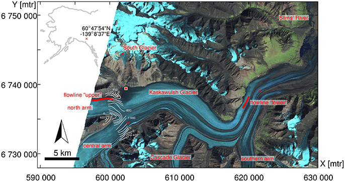
Figure 2. False color composite of a SPOT5 acquisition taken on the 4th of August 2015 of the lower part of Kaskawulsh Glacier, together with the flowlines used in this study. The square indicates the location of a glacier-dammed lake, the circle indicates the position of the automatic weather station, and the two crosses indicate dismantled dGPS stations. The flow direction is from left to right. In the confluence of Northern and Central Arm the local (bedrock) topography is illustrated with white isohypses, they have an interval of 200 m and are redrawn from Dewart (1968).

The acquisitions of the SPOT5 Take5 campaigns where taken from the 11th of July 2015 till the 8th of September 2015. Imagery was collected with an interval of 5 days, with an exception for the 31st of May and the 24th of August. The imagery is multispectral (green, red, NIR, and SWIR), the pixel resolution is 10 m and the imagery has an extent of roughly 62 km.

4. Method

In this section, the implementation of our approach based on the above methodological background is laid out. Our implementation comprises of two approaches and thrives on data reduction, through the simplification of the spatial domain to a glacier flowline. By doing so, we assume the flowline does not change, i.e., the flow direction stays constant over time. Hence motion out of the vertical plane through the flowline will result in a reduced estimation of speed. This might be the case when tributaries surge, or competing flows interfere. Normally, the dominant change in velocity is due to sliding, hence mainly the magnitude of velocity changes, not or much less its direction.

4.1. Trajectory

In order to obtain the flowline that is used to slice through the data-cube, we rely on traditional image matching. Alternatively, it is possible to estimate a centerline through GIS routines based on a DEM (Kienholz et al., 2014; Machguth and Huss, 2014; Le Moine and Gsell, 2015) or glacier outlines, but for instance on flat glaciers such an estimated line may not align well with the flow. Therefore, in our implementation, out of a collection of imagery, good pairs are selected that have a minimum of cloud cover and strong visual contrast to do image matching and extract a velocity field. Specifically, we used two image pairs, one from spring and one from autumn, and after local median filtering the two velocity fields are combined by taking the mean. The resulting vector field is then used to estimate a trajectory, given a seed point (see Figure 3).

FIGURE 3

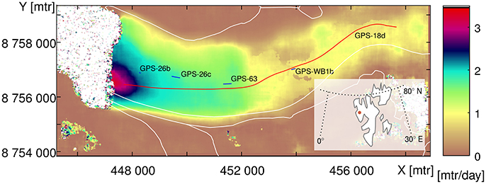
Figure 3. Flow magnitude of Kronebreen, derived from SPOT5 Take5 imagery (merge between spring and autumn speed, see text). In red the flowline, used for this study is highlighted. The blue lines indicate the travel path of the GPS stakes, its data is kindly provided by J. Kohler, Norwegian Polar Institute.

4.2. Space-Time

This estimated trajectory is the reference line for the image data sampling and tracking. Two different strategies can now be exploited, one based on the pattern given by the imagery and one based on features within the imagery.

The construction of the image stack, i.e., of the temporal axis, is done by sampling the Red, Green, and NIR image bands at 10 m spacings along the flowline (i.e., above trajectory). As we are interested in local features, and less so in the absolute values, a high-pass filter is applied onto this image, prior to the sampling. The flowline is not aligned with the pixel array, thus bi-linear interpolation is used for the sampling. Then for every time instance, which has a fixed time interval of 5 days in our case, a line of high-frequency interpolated intensities is added to the stack, forming a space-time slice. Manual delineation is applied onto the space-time image to estimate the temporal velocity change. Features are tracked by clicking several polylines within the space-time slice. The slope of a line segment from such a polyline is a direct estimate of the velocity, see Equation (4). From this it becomes clear that the longer the time interval (i.e., the length of the time-domain segment), the more accurate the slope (i.e., velocity estimation) is.

A second strategy is based on image features. First, the Harris feature detector (Harris and Stephens, 1988), creates an energy field which is thresholded in absolute sense, resulting however in clustering (Brown et al., 2005). Therefore, a moving window is used, including the local maximum, consequently, features are more spread out over the scene, see Figure 4. For robustness, the sub-pixel localization is done through a center-of-gravity estimation (van Assen et al., 2002), and not a parabolic fitting of some sort. The resulting features are not necessarily strictly on the flowline, thus a buffer is created to select features close to the flowline. This procedure is applied to every image. From this collection of features within the image collection, connections need to be made. Every feature recorded at one time instance can be connected with another feature. Many combinations are possible, therefore a rule needs to be implemented, to do so. This assignment problem is solved by a simple implementation. The search space in time is set to a certain upper limit at three times the mean speed at that point to account for speed changes, plus an additional 7.5 m to account for potential co-registration errors. Thus, per unit of time one is limited to look up to a certain distance away from the feature, beginning with a master image and a collection of features in it, and a slave image where features are searched for. Then, for each feature in the slave image, the position is reversed with a tracer to get to the position at the time of the master image. Thereby, the same velocity field as used for extraction of the flowline is utilized. The tracer estimates the position of the feature in the master-image. When this estimated position is at close proximity to a master-image feature, it is considered a candidate connection. The specification of close proximity is depended on the quality of the velocity field and the magnitude of variability in speed. Nonetheless, multiple candidate connections can be established, therefore a descriptor, a local binary pattern (Heikkilä et al., 2009), is used to assess the amount of similarity and validity of a connection. Thus, our assignment is implemented by several levels. The use of a moving window ensures that features are more evenly distributed. Then the potential feature-set is reduced through back-tracking, and the local binary pattern serves as a final hard classification rule.

FIGURE 4

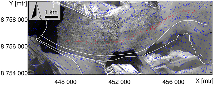
Figure 4. SPOT5 imagery taken over Kronebreen at the 29th of April 2015. The blue dots highlight the Harris corner detections, the red dots indicate Harris interest points within the buffer of the flowline, which are used for the tracking. The white lines are glacier outlines from Nuth et al. (2013).

5. Results

5.1. Kaskawulsh, St. Elias, Yukon

Kaskawulsh Glacier lies within the St. Elias mountain range, Yukon. It is a 70 km long temperate glacier which originates from the Kluane icefield. The annual variability of flow speed can at some places be in the order of 25% (Waechter et al., 2015). The overall annual cumulative speed, or displacement per year, has not changed considerably throughout the last decades. From all 29 SPOT5 Take5 acquisitions, only seven are to a large extent cloud-covered, the rest are cloudless or have minor clouds scattered over the scene. This dataset is therefore ideal to implement the pattern-method, as described in Section 4.2, where imagery is stacked and a vertical slice is analyzed.

A continuous measurement campaign of several dGPS stations has been deployed for 7 years on Kaskawulsh Glacier. However, the campaign ended a year prior to the 2015 Take5 mission. Dependent on the season, different velocity patterns occurred. At the start of the melt season, velocities increase and this increase propagates up-glacier as time progresses. In winter season the velocities decrease again, but this velocity change propagates down-glacier over time (Herdes, 2014, Luke Copland, pers. comm.). Therefore, it is of interest to not only investigate one point at high precision, but to also study the spatial pattern of the seasonal flow evolution. Another network of GPS-stations is installed in the vicinity of a glacier dammed lake (see the square in Figure 2). These instruments are set out to look at short-term drainage processes. At the lake border the glacier flow is very limited. In addition, on this glacier section, or on the neighboring South Glacier almost no visually coherent features can be found that can be tracked over time. Therefore, no direct verification data is available over the Kaskawulsh site. However the cloud cover is very much limited, and this case study is thus meant to demonstrate our pattern method for upcoming dense time-series of optical data.

Two flowlines were sampled on the Kaskawulsh Glacier. The first flowline (named “upper”) leads over a crevasse field that, due to its shading and shadowing, is visible over the full time period. Furthermore, it is in proximity of the location where formerly an installation of a dGPS has been recording. Its space-time image is illustrated in Figure 5. In our space-time visualization speed-ups appear as inclinations tilting into flow direction (here: right), and slow-downs as tiltings against flow direction, i.e., toward the vertical. A change in displacement is clearly visible starting in mid-May, then velocity slowly declines throughout the summer.

FIGURE 5

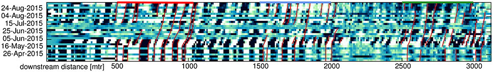
Figure 5. Space-time image from SPOT5 Take5 imagery of flowline “upper” of Kaskawulsh Glacier, as in Figure 2. The white-green-black patterns are the high frequency intensities on the drawn flowline. Because many features are discontinuous, tracking is done on different section of the flowline. The horizontal colored bars on top of the figure indicate these sections of displacement estimates, which colors correspond to the velocity estimates in Figure 7.

Over the full 3 km extracted, the glacier seems to move as a bulk. This is more clearly observable when features are tracked manually and not interpreted. These are the red lines superimposed onto the image, following features along the space-time slice. Every segment of these polylines has a coordinate in space and time, consequently, its slope gives the velocity over this period. Estimates over such time intervals are plotted in Figure 5 as horizontal lines. The lines following features are subdivided in three different segments, and color coded, to assess the reliability and spread of the velocity estimates. Their timing and magnitude seem to be in accordance with each other. A multiple annual mean seasonal velocity estimate from a dGPS station from the nearby Central arm is also plotted in this figure, as a thicker gray line. The magnitude of the late-winter velocities seems to be higher for this station, than the sampled flow line. This can be due to the difference in depth, as the sampled line is in a shallower part then the dGPS station, see Figure 2. The factor between different magnitudes in glacier speed is due to the position of the flowline, which is in a shearing zone with high differential motion, see Figure 3B in Waechter et al. (2015). The mean velocity in the spring season covers both slow and high speeds, and is therefore difficult to assess. The fall season seems again to be in accordance with our estimate, however the estimates are noisy.

The second flowline is named “lower” like the dGPS station which has been recording for several years, but was dismantled a year before the Take5 campaign. The flowline is situated over a crevasse field, in the middle of the glacier branch that is also connected to the “upper” flowline. The space-time slice over this flow line is illustrated in Figure 6. Its conversion to velocities is illustrated in Figure 7. In the background is the temperature record from an automatic weather station for South Glacier, which is at 2,280 masl. The “upper” profile is closer to South Glacier and at an approximate elevation of 1,750 masl, while the “lower” flowline is situated at around 1,150 masl. Nevertheless, over a short period of time the temperature increases in late winter/early spring. This warming results in more meltwater input into the hydrological network. Due to the meteorological lapse rate, melt occurs later at higher elevations. This effect is observable when the timing of speed-up at the “upper” and “lower” locations are compared to each other, see the vertical lines in Figure 7. The “lower” flowline experiences an earlier speed-up, roughly 10 days earlier. Such an effect has been observed in the dGPS campaign in the years prior to the Take5 campaign (Darling, 2012; Herdes, 2014), and our estimates seem to be able to observe the timing of such dynamics. Furthermore, in the beginning of July the glacier dammed lake drained (Gwenn Flowers, pers. comm.), however no speed change is observable for this period in our estimates at point “lower”.

FIGURE 6

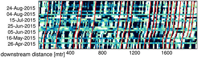
Figure 6. Space-time image from SPOT5 Take5 imagery of flowline “lower” of Kaskawulsh Glacier, as illustrated in Figure 2. In the background the white-green-black color scheme corresponds to high-pass filtered intensities of the image at the position of the flowline. The red lines try to follow features within the slice and are used in the velocity estimates in Figure 7.

FIGURE 7

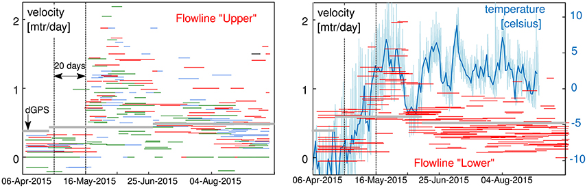
Figure 7. Velocity estimation at different positions on the flowline of Kaskawulsh Glacier. These curves are integrated from the lines drawn in Figure 5. Colors correspond to the segments shown on top of Figures 5, 6. The 5 min interval temperature data is in light blue and its daily mean in darker blue. The automatic weather station data is kindly provided by G. Flowers, Simon Fraser University. The dark gray horizontal lines are the multi-year seasonal average of nearby GPS stations, data from L. Copland, University of Ottawa.

5.2. Kronebreen, Svalbard

Kronebreen is a tidewater glacier near Ny-Ålesund on Svalbard, it is an outlet glacier that transports ice from the 300km² Holtedahlfonna and the 70km² Infantfonna icefield into the ocean. Its lower part is constrained by a narrow valley of roughly 5 km wide, see Figures 3, 4. The flow is all-year round at a high speed of a couple of meters per day (Kääb et al., 2005; Schellenberger et al., 2016). From the 30 SPOT5 Take5 acquisitions taken over Kronebreen, only five where cloud free. Especially July 2015 was unusually cloudy. Hence, in order to have a more useful dense image stack, cloud-free Landsat 8 imagery was included to form a time series together with the SPOT5 Take5 data. Due to Landsat 8 s continuous sampling strategy and the high latitude of Svalbard, images were collected from different orbit paths and different times of the day, ranging from 04:47 to 23:52 local time. The varying sun angles changed the visual appearance of the images heavily. Since 2009, several stand-alone single-frequency GPS receivers have been installed on Kronebreen. In our case, the positional estimates used are daily averages of four GPS stakes.

A total of 50 Landsat 8 and SPOT5 images were used for the extraction of velocity over the Kronebreen glacier. For this case study the feature method, as described in Section 4.2, is used. This is done because the pattern method, using the intensities directly is not sufficient. Such a pattern stack is illustrated in Figure 8, to illustrate the complications. Within the space-time image slice of Figure 8, the features are clearly observable; however this is also a weakness. For example, when over a period clouds were present and movement has been significant, it is difficult to follow the correctly corresponding crevasse feature, as they all have a self-similar alternating pattern. This is the case in July, which was a cloudy month, resulting in gray noise without coherent texture. In addition, co-registration errors, because of different acquisition angles (Altena and Kääb, 2017), can potentially cause bending/tilting. Therefore, in this section we use the feature based method.

FIGURE 8

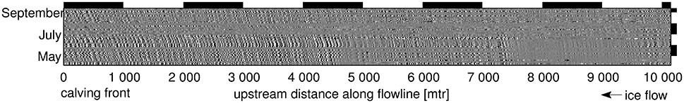
Figure 8. Space-time image slice pattern from SPOT5 Take5 imagery of Kronebreen. The black and white patterns are high-pass filtered intensities. The flowline used to slice the data-cube is illustrated in Figure 3. Flow direction is from right to left of the slice.

The Harris corner detector had a moving window with an extent of 300 m, intensity corners were selected with a regular threshold setting (sensitivity factor, α = 0.04). First, the correspondence problem was solved only with a neighborhood constraint, i.e., if a feature was close by (within 7.5 m), a connection was made. This resulted in a well-populated space-time slice, as illustrated in dark gray within Figure 9. Though coherent tilts in the spatial and temporal domain are observable, outliers existed. A descriptor was therefore included into the selection program and multiple candidates could be tested. This resulted in a harder selection, though more reliable, and the resulting trajectories are illustrated in red within Figure 9. In addition to the estimated trajectories, the GPS measurements (position see Figure 3) are illustrated as well. Though the spatio-temporal trajectories from the optical dataset are sparse, there is general agreement with the GPS trajectories (Figure 10). In July a speed-up occurred, and was recorded by the GPS, is not apparent in our velocity estimates due to cloud cover. The spread of the estimates is also observable, but when multiple estimates are present, when sufficient estimates are present they do align with the measured GPS speed. Nonetheless, outliers exist. In order to be of use for analysis, the samples need to be of considerable size and trend estimators need to be robust against heavy tails.

FIGURE 9

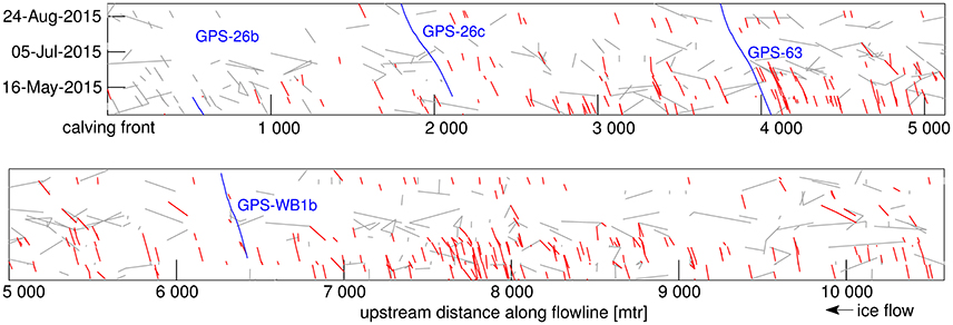
Figure 9. Space-time image of the Kronebreen flowline illustrated in Figure 2 in red. The filtered correspondences are in gray. Trajectories of the GPS stakes are shown in blue.

FIGURE 10

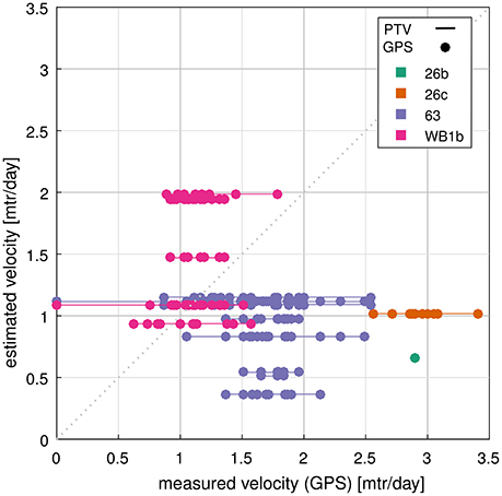
Figure 10. Velocity measurements of the GPS on Kronebreen are plotted in different colors and are indicated by the dots. These measurements are set against th the estimated velocities of features, as in Figure 3. These estimates cover a certain time span and are therefore illustrated as a line. Only estimates within a spatio-temporal neighborhood of 200 m of the GPS's are included and shown.

6. Discussion

In both case studies, our approach reveals reasonable and validated seasonal and spatial variations in glacier speed. We simplify the space-time domain along flow-lines which results in a reduction of the spatial coverage in comparison to classical image matching approaches. However, the temporal resolution becomes maximum in our approach (i.e., all available images are included) such that short events become visible in ways that would be difficult or computationally intensive to identify using traditional image matching.

The SPOT5 Take5 dataset, as well as the Landsat imagery will have geo-referencing errors and orthorectification errors. The absolute localization was refined through co-registering all images to a Landsat scene, while relatively the SPOT5 data where registered on sub-pixel level (Hagolle et al., 2015). This will have an effect on the absolute geolocation, but this is not of interest in this study. Relative to each other, the images will have some remaining co-registration inaccuracies. In this study, we are using tens of images, hence the co-registration inaccuracies will appear as small roughness of the time-domain features, leaving them displayed as a whole. When the temporal baseline increases the patterns start to emerge above the co-registration noise, i.e., roughness of the space-time features.

In the “upper” section of the Kaskawulsh Glacier velocity estimates have been subdivided into three sections. Although some spread occurs in the velocity estimates, the timing of the increase in speed is clear and in accordance with each other. The velocity estimates have different spans of time, hence fusion of such estimates into a coherent time-series can be complicated. Furthermore, the pattern extraction is manual and thrives on visual interpretation. Attempts for automatic procedures for such data did not work out. Consequently, our method is clearly an exploratory tool and no replacement for image matching. Nevertheless, it can be of help in selection the appropriate set of images in a large image collection or for identifying special dynamic events.

The combination of a Harris-corner detection and center-of-mass sub-pixel estimation is a computationally fast detector. However, due to this choice, a compromise is made with the localization of the corner. For example, the Plessy-detector (Noble, 1988) might be more precise in its estimate for “cornerness” at every pixel. The Föstner-detector (Förstner and Gülch, 1987) directly estimates corners at sub-pixel level through ordinary least squares adjustment, but is computationally more intensive. A similar sub-pixel Harris detector, also using least squares adjustment (Zhu et al., 2007), was implemented, but seemed sensitive to noise and outliers. It is this repeatability of a detector which is of more importance for our application, and for blur (thin clouds) and noise (loss of visual coherence) these properties seem to be relatively good for the Harris-detector (Montero et al., 2010).

In the summer period, when the speed up of Kronebreen occurred, almost no cloudless images are available for the year studied. The additional Landsat imagery was thus only helpful to a limited extent. This can be due to the simple feature descriptor used in this study. The sun angle heavily changed the appearance of the crevasse field of Kronebreen. More advanced feature descriptors, such as for example SIFT (Lowe, 2004) or LIOP (Wang et al., 2011), might be able to better describe the feature in such instances. In such implementation, the difference with traditional image matching will reduce, and similar limitations will start to occur. Nevertheless, illumination-invariant image descriptors reduce miss-assignments of correspondences and with the help of robust neighborhood statistics, one might be able to produce a detailed time-series. For the Kronebreen case, such an approach might still not be able to extract the speed-up occurring in summer as cloud cover stays a problem, which cannot be tackled with optical remote sensing data. Eventually thus, the optical flow methods demonstrated here could be applied to merged optical and SAR data.

One extension to enhance robustness is by incorporating image matching. Annual displacements can be estimated from two selected scenes, which relates to two end-nodes on a space-time representation. These end-nodes can be used to constrain the path-finding within the space-time imagery.

7. Prospect

The key strength of this method is the ability to explore the timing of glacier speed variations from massive image stacks without the need of matching image pairs. Image matching is computationally costly when applied to large data sets and prone to specific problems, for instance related to image selection or assignment of corresponding patterns. In contrast, image stacks and space-time slices can be extracted and visualized fast and efficient. We therefore envisage a range of three potential application scenarios for the approaches introduced here:

First, our methods offer a simple alternative technique for visualizing glacier speed variations over time from massive stacks of repeat images. In view of the wealth of current and in particular upcoming satellite data, it might not be sufficient to use only classical visualization approaches, such as vector fields or image animations (Paul, 2015).

Second, our methods can be used to visualize the space-time content of a massive series of repeat images in order to select a subset of the most suitable (cloud-free) image pairs to apply image matching to, manually or automatically. For instance, suitable matching scenes become well-visible in our space-time slices. Or, a higher density of matching pairs can be selected around variations in speed as visible in the deviations of space-time features from straight lines in the time domain, leading to some kind of adaptive selection of matching pairs.

Third, our methods can be used to directly derive glacier speed and its variation over time by extracting and analyzing space-time features, as demonstrated for both case studies. Again, (near-)future amounts of satellite data suitable to monitor glacier flow might simply be too large to apply classical image matching methods.

8. Conclusion

This case study explores the potential of increased satellite revisit time in combination with tracking approaches from other scientific fields, optical flow, and particle tracking velocimetry, for the monitoring of glacier speed. Our methods explored the simplification of current approaches through data reduction by means of flowlines. This approach is new, though it has been applied to other glaciological applications, such as glacier snout extent (Usset et al., 2015).

Two technical approaches were highlighted, including pattern-based and feature-based, and were applied to two glaciers. In both studies, the seasonal pattern and timing of the summer acceleration could be identified. The strategies for connecting features or finding orientation within the space-time data were primitive in the context of this study. However, there is potential knowledge within the research field of computer vision or fluid mechanics available to automate robust procedures to mate features or estimate orientation.

This study also shows the potential of our approaches for multi-sensor integration. The velocity of Kronebreen was extracted from acquisitions of different satellites. In addition, the feature based methodology seemed to be less hindered by cloud cover, then traditional image matching. This promise opens the possibility for high resolution imagery with daily revisit time. Hence, our methodology is relevant for Sentinel-2, when the companion-satellite constellation is in full operation. However, upcoming constellations of small satellites (e.g., Planet, UrtheCast, Blacksky, …) might even enhance the opportunity to monitor the inter-seasonal dynamics of glaciers using the approaches evaluated and demonstrated here.

Author Contributions

BA and AK initiated the study. BA designed the structure, developed, and implemented the methodology. Both authors interpreted the results and wrote the article.

Conflict of Interest Statement

The authors declare that the research was conducted in the absence of any commercial or financial relationships that could be construed as a potential conflict of interest.

Acknowledgments

We would like to thank Jack Kohler for providing us the GPS data over Kronebreen and Gwenn Flowers for the AWS data over South Glacier. Furthermore, we thank Luke Copland for discussions about the flow dynamics of Kaskawulsh Glacier. We are also grateful to three referees and the editor Alun Hubbard for their constructive comments that certainly helped to improve the paper. We also thank Shae Frydenlund for improving the English language of an early version of this contribution. This study is funded by the European Research Council under the European Union's Seventh Framework Programme grant agreement no. 320816 and the ESA project Glaciers_cci (4000109873/14/I-NB). We are very grateful to ESA and the EU Copernicus program for free provision of the SPOT5 imagery.

References

Adelson, E., and Bergen, J. (1985). Spatiotemporal energy models for the perception of motion. J. Opt. Soc. Am. A 2, 284–299.

PubMed Abstract | Google Scholar

Ahn, Y., and Howat, I. (2011). Efficient automated glacier surface velocity measurement from repeat images using multi-image/multichip and null exclusion feature tracking. IEEE Trans. Geosci. Remote Sens. 49, 2838–2846. doi: 10.1109/TGRS.2011.2114891

CrossRef Full Text | Google Scholar

Altena, B., and Kääb, A. (2017). Elevation change and improved velocity retrieval using orthorectified optical satellite data from different orbits. Remote Sens. 9:300. doi: 10.3390/rs9030300

CrossRef Full Text | Google Scholar

Armstrong, W. H., Anderson, R. S., Allen, J., and Rajaram, H. (2016). Modeling the WorldView-derived seasonal velocity evolution of Kennicott glacier, Alaska. J. Glaciol. 62, 763–777. doi: 10.1017/jog.2016.66

CrossRef Full Text | Google Scholar

Baker, S., Scharstein, D., Lewis, J., Roth, S., Black, M., and Szeliski, R. (2011). A database and evaluation methodology for optical flow. Int. J. Comp. Vis. 92, 1–31. doi: 10.1007/s11263-010-0390-2

CrossRef Full Text | Google Scholar

Barron, J., Fleet, D., and Beauchemin, S. (1994). Performance of optical flow techniques. Int. J. Comp. Vis. 12, 43–77.

Google Scholar

Berthier, E., Vadon, H., Baratoux, D., Arnaud, Y., Vincent, C., Feigl, K., et al. (2005). Surface motion of mountain glaciers derived from satellite optical imagery. Remote Sens. Environ. 95, 14–28. doi: 10.1016/j.rse.2004.11.005

CrossRef Full Text | Google Scholar

Bindschadler, R., Scambos, T., Choi, H., and Haran, T. (2010). Ice sheet change detection by satellite image differencing. Remote Sens. Environ. 114, 1353–1362. doi: 10.1016/j.rse.2010.01.014

CrossRef Full Text | Google Scholar

Brown, M., Szeliski, R., and Winder, S. (2005). “Multi-image matching using multi-scale oriented patches,” in IEEE Conference on Computer Vision and Pattern Recognition, Vol. 1 (San Diego, CA), 510–517.

Google Scholar

Bruce, V., Green, P., and Georgeson, M. (2003). Visual Perception: Physiology, Psychology, & Ecology. New York, NY: Psychology Press.

Google Scholar

Chen, Y., Zhao, Z., Liu, L., and Li, H. (2011). Automatic tracking and measurement of the motion of blood cells in microvessels based on analysis of multiple spatiotemporal images. Meas. Sci. Technol. 22:045803. doi: 10.1088/0957-0233/22/4/045803

CrossRef Full Text | Google Scholar

Darling, S. (2012). Velocity Variations of the Kaskawulsh Glacier, Yukon Territory, 2009-2011. Master's thesis, University of Ottawa.

Debella-Gilo, M., and Kääb, A. (2011). Sub-pixel precision image matching for measuring surface displacements on mass movements using normalized cross-correlation. Remote Sens. Environ. 115, 130–142. doi: 10.1016/j.rse.2010.08.012

CrossRef Full Text | Google Scholar

Debella-Gilo, M., and Kääb, A. (2012). Measurement of surface displacement and deformation of mass movements using least squares matching of repeat high resolution satellite and aerial images. Remote Sens. 4, 43–67. doi: 10.3390/rs4010043

CrossRef Full Text | Google Scholar

Dewart, G. (1968). Seismic Investigation of Ice Properties and Bedrock Topography at the Confluence of Two Glaciers, Kaskawulsh Glacier, Yukon Territory, Canada. Technical Report 27, Institute of Polar Studies, The Ohio State University.

Google Scholar

Fahnestock, M., Scambos, T., Moon, T., Gardner, A., Haran, T., and Klinger, M. (2015). Rapid large-area mapping of ice flow using Landsat 8. Remote Sens. Environ. 185, 84–94. doi: 10.1016/j.rse.2015.11.023

CrossRef Full Text | Google Scholar

Förstner, W., and Gülch, E. (1987). “A fast operator for detection and precise location of distinct points, corners and centres of circular features,” in Proc. ISPRS Intercommission Conference on Fast Processing of Photogrammetric Data (Interlaken), 281–305.

Freeman, W. T., and Adelson, E. H. (1991). The design and use of steerable filters. IEEE Trans. Pattern Anal. Mach. Intell. 13, 891–906.

Google Scholar

Guezennec, Y., Brodkey, R., Trigui, N., and Kent, J. (1994). Algorithms for fully automated three-dimensional particle tracking velocimetry. Exp. Fluids 17, 209–219.

Google Scholar

Hagolle, O., Sylvander, S., Huc, M., Claverie, M., Clesse, D., Dechoz, C., et al. (2015). SPOT-4 (take 5): simulation of Sentinel-2 time series on 45 large sites. Remote Sens. 7, 12242–12264. doi: 10.3390/rs70912242

CrossRef Full Text | Google Scholar

Harris, C., and Stephens, M. (1988). “A combined corner and edge detector,” in Alvey Vision Conference, Vol. 15 (Manchester), 147–151.

Google Scholar

Heid, T., and Kääb, A. (2012). Evaluation of existing image matching methods for deriving glacier surface displacements globally from optical satellite imagery. Remote Sens. Environ. 118, 339–355. doi: 10.1016/j.rse.2011.11.024

CrossRef Full Text | Google Scholar

Heikkilä, M., Pietikäinen, M., and Schmid, C. (2009). Description of interest regions with local binary patterns. Pattern Recognit. 42, 425–436. doi: 10.1016/j.patcog.2008.08.014

CrossRef Full Text | Google Scholar

Heitz, D., Mémin, E., and Schnörr, C. (2010). Variational fluid flow measurements from image sequences: synopsis and perspectives. Exp. Fluids 48, 369–393. doi: 10.1007/s00348-009-0778-3

CrossRef Full Text | Google Scholar

Herdes, É. (2014). Evolution of Seasonal Variations in Motion of the Kaskawulsh Glacier, Yukon Territory. Master's thesis, University of Ottawa.

Horn, B., and Schunck, B. (1981). “Determining optical flow,” in 1981 Technical Symposium East (Washington, DC: International Society for Optics and Photonics), 319–331.

Huss, M., Voinesco, A., and Hoelzle, M. (2013). Implications of climate change on Glacier de la Plaine Morte, Switzerland. Geogr. Helv. 68, 227–237. doi: 10.5194/gh-68-227-2013

CrossRef Full Text | Google Scholar

Jähne, B. (1993). Spatio-Temporal Image Processing: Theory and Scientific Applications. Heidelberg: Springer. doi: 10.1007/3-540-57418-2

CrossRef Full Text | Google Scholar

Kääb, A. (2005). Remote Sensing of Mountain Glaciers and Permafrost Creep, Vol. 48. Zürich: Schriftenreihe Physische Geographie.

Kääb, A., Lefauconnier, B., and Melvold, K. (2005). Flow field of Kronebreen, Svalbard, using repeated Landsat 7 and ASTER data. Ann. Glaciol. 42, 7–13. doi: 10.3189/172756405781812916

CrossRef Full Text | Google Scholar

Kääb, A., and Vollmer, M. (2000). Surface geometry, thickness changes and flow fields on creeping mountain permafrost: automatic extraction by digital image analysis. Permafrost Periglacial Process. 11, 315–326. doi: 10.1002/1099-1530(200012)11:4<315::AID-PPP365>3.0.CO;2-J

CrossRef Full Text | Google Scholar

Kääb, A., Winsvold, S., Altena, B., Nuth, C., Nagler, T., and Wuite, J. (2016). Glacier remote sensing using Sentinel-2. part I: Radiometric and geometric performance, and application to ice velocity. Remote Sens. 8, 598. doi: 10.3390/rs8070598

CrossRef Full Text | Google Scholar

Kienholz, C., Rich, J., Arendt, A., and Hock, R. (2014). A new method for deriving glacier centerlines applied to glaciers in Alaska and northwest Canada. Cryosphere 8, 503–519. doi: 10.5194/tc-8-503-2014

CrossRef Full Text | Google Scholar

Le Moine, N., and Gsell, P.-S. (2015). A graph-based approach to glacier flowline extraction: an application to glaciers in Switzerland. Comp. Geosci. 85, 91–101. doi: 10.1016/j.cageo.2015.09.010

CrossRef Full Text | Google Scholar

Lowe, D. (2004). Distinctive image features from scale-invariant keypoints. Int. J. Comp. Vis. 60, 91–110. doi: 10.1023/B:VISI.0000029664.99615.94

CrossRef Full Text | Google Scholar

Luttman, A., Bollt, E., Basnayake, R., Kramer, S., and Tufillaro, N. (2013). A framework for estimating potential fluid flow from digital imagery. Chaos 23:033134. doi: 10.1063/1.4821188

PubMed Abstract | CrossRef Full Text | Google Scholar

Maas, H., Gruen, A., and Papantoniou, D. (1993). Particle tracking velocimetry in three-dimensional flows. Exp. Fluids 15, 133–146.

Google Scholar

Machguth, H., and Huss, M. (2014). The length of the world's glaciers–a new approach for the global calculation of center lines. Cryosphere 8, 1741–1755. doi: 10.5194/tc-8-1741-2014

CrossRef Full Text | Google Scholar

Montero, A., Stojmenovic, M., and Nayak, A. (2010). “Robust detection of corners and corner-line links in images,” in IEEE 10th International Conference on Computer and Information Technology (Bradford), 495–502.

Google Scholar

Noble, J. (1988). Finding corners. Image Vis. Comput. 6, 121–128.

Google Scholar

Nuth, C., Kohler, J., König, M., Deschwanden, A. V., Hagen, J., Kääb, A., et al. (2013). Decadal changes from a multi-temporal glacier inventory of Svalbard. Cryosphere 7, 1603–1621. doi: 10.5194/tc-7-1603-2013

CrossRef Full Text | Google Scholar

Paul, F. (2015). Revealing glacier flow and surge dynamics from animated satellite image sequences: examples from the Karakoram. Cryosphere 9, 2201–2214. doi: 10.5194/tc-9-2201-2015

CrossRef Full Text | Google Scholar

Planet Team (2017). Planet Application Program Interface: In Space for Life on Earth. San Francisco, CA.

Prasad, A., Adrian, R., Landreth, C., and Offutt, P. (1992). Effect of resolution on the speed and accuracy of particle image velocimetry interrogation. Exp. Fluids 13, 105–116.

Google Scholar

Raffel, M., Willert, C., Wereley, S., and Kompenhans, J. (2013). Particle Image Velocimetry: A Practical Guide. Heidelberg: Springer.

Google Scholar

Scambos, T., Dutkiewicz, M., Wilson, J., and Bindschadler, R. (1992). Application of image cross-correlation to the measurement of glacier velocity using satellite image data. Remote Sens. Environ. 42, 177–186.

Google Scholar

Scambos, T., Fahnestock, M., Moon, T., Gardner, A., and Klinger, M. (2016). Global Land Ice Velocity Extraction from Landsat 8 (GoLIVE), Version 1. Boulder, CO: NSIDC: National Snow and Ice Data Center.

Schellenberger, T., Van Wychen, W., Copland, L., Kääb, A., and Gray, L. (2016). An inter-comparison of techniques for determining velocities of maritime arctic glaciers, Svalbard, using Radarsat-2 wide fine mode data. Remote Sens. 8:785. doi: 10.3390/rs8090785

CrossRef Full Text | Google Scholar

Sveen, J., and Cowen, E. (2004). “Chapter 1: quantitative imaging techniques and their application to wavy flows,” in PIV and Water Waves, Vol. 9, eds J. Grue, P. L.-F. Liu, and G. K. Pedersen (World Scientific Publishing), 1–49.

Tuytelaars, T., and Mikolajczyk, K. (2008). Local invariant feature detectors: a survey. Found. Trends. Comp. Graph. Vis. 3, 177–280. doi: 10.1561/0600000017

CrossRef Full Text | Google Scholar

Usset, J., Maity, A., Staicu, A.-M., and Schwartzman, A. (2015). Glacier terminus estimation from Landsat image intensity profiles. J. Agric. Biol. Environ. Stat. 20, 279–298. doi: 10.1007/s13253-015-0207-4

CrossRef Full Text | Google Scholar

van Assen, H., Egmont-Petersen, M., and Reiber, J. (2002). Accurate object localization in gray level images using the center of gravity measure: accuracy versus precision. IEEE Trans. Image Process. 11, 1379–1384. doi: 10.1109/TIP.2002.806250

PubMed Abstract | CrossRef Full Text | Google Scholar

Vogel, C., Bauder, A., and Schindler, K. (2012). “Optical flow for glacier motion estimation,” in Proceedings of the 22nd ISPRS Congress, Vol. 25 (Melbourne, VIC).

Google Scholar

Wadhwa, N., Rubinstein, M., Durand, F., and Freeman, W. (2013). Phase-based video motion processing. ACM Trans. Graph. 32:80. doi: 10.1145/2461912.2461966

CrossRef Full Text | Google Scholar

Waechter, A., Copland, L., and Herdes, E. (2015). Modern glacier velocities across the Icefield Ranges, St Elias Mountains, and variability at selected glaciers from 1959 to 2012. J. Glaciol. 61, 624–634. doi: 10.3189/2015JoG14J147

CrossRef Full Text | Google Scholar

Wang, Z., Fan, B., and Wu, F. (2011). “Local intensity order pattern for feature description,” in IEEE International Conference on Computer Vision (Barcelona), 603–610.

Google Scholar

Warren, S. (1982). Optical properties of snow. Rev. Geophys. Space Phys. 20, 67–89.

Google Scholar

Zhu, Q., Wu, B., and Wan, N. (2007). A sub-pixel location method for interest points by means of the Harris interest strength. Photogrammetric Rec. 22, 321–335. doi: 10.1111/j.1477-9730.2007.00450.x

CrossRef Full Text | Google Scholar